Article

An EMD-LSTM Deep Learning Method for Aircraft Hydraulic System Fault Diagnosis under Different Environmental Noises

1
College of Automation Engineering, Nanjing University of Aeronautics and Astronautics, Nanjing 210016, China
2
College of Mechanical and Electrical Engineering, Nanjing University of Aeronautics and Astronautics, Nanjing 210016, China
*
Author to whom correspondence should be addressed.
Aerospace 2023, 10(1), 55; https://doi.org/10.3390/aerospace10010055
Submission received: 28 November 2022 / Revised: 18 December 2022 / Accepted: 20 December 2022 / Published: 5 January 2023

Abstract

:
Aircraft hydraulic fault diagnosis is an important technique in aircraft systems, as the hydraulic system is one of the key components of an aircraft. In aircraft hydraulic system fault diagnosis, complex environmental noises will lead to inaccurate results. To address the above problem, hydraulic system fault detection methods should be capable of noise resistance. Previous research has mainly focused on noise-free conditions and many effective approaches have been proposed; however, in real-world aircraft flying conditions, the aircraft hydraulic system often has strong and complex noises. The methods proposed may not have good fault detection results in such a noisy environment. According to the situation, this work focuses on aircraft hydraulic system fault classification under the influence of a hydraulic working environment with Gaussian white noise. In order to eliminate the noise interference and adapt to the actual noisy environment, a new aircraft hydraulic fault diagnostic method based on empirical mode deposition (EMD) and long short-term memory (LSTM) is presented. First, the hydraulic system is constructed by AMESIM. One normal state and five fault states are considered in this paper. Eight-channel signals of different states are collected for network training and testing. Second, the EMD method is used to obtain the different intrinsic mode functions (IMFs) of the signals. Third, principal component analysis (PCA) is used to obtain the main component of the IMFs. Fourth, three different LSTM methods are chosen to compare and the best structure that is chosen is the gate recurrent unit (GRU). After that, the network parameters are optimized. The results under different noise environments are given. Then, a comparison between the EMD-GRU with several different machine learning methods is considered, and the result shows that the method in this paper has a better anti-noise effect. Therefore, the proposed method is demonstrated to have a strong ability of fault diagnosis and classification under the working noises based on the simulation results.

1. Introduction

The hydraulic system is an important part of an aircraft, which is the key to ensuring the safety of both the aircraft and its passengers. Aircraft hydraulic systems account for a large proportion of aircraft maintenance work, the failures of aircraft hydraulic systems make up about 30% of total mechanical failures, and their maintenance accounts for one-third of the total mechanical maintenance [1].
Therefore, the hydraulic system has a crucial impact on the reliability of the whole aircraft system, and effective fault diagnostic methods should be presented to ensure the safe operation of the aircraft. In order to ensure the safety of the hydraulic system, numerous fault diagnostic methods are proposed. Early research can be divided into two categories, that is, experience-based diagnostic methods [2,3,4] and model-based diagnostic methods [5,6]. However, with these methods, it is hard to distinguish all the fault types in a hydraulic system, and it is difficult to establish a model because of the complexity of the aircraft hydraulic system. Therefore, a lot of advanced approaches to deep-learning-based fault diagnosis and feature extraction have been proposed [7,8,9,10] in recent years. Among these methods, the LSTM-based methods have a better processing ability to deal with timing signals.
Long short-term memory (LSTM) neural network is an improved recurrent neural network (RNN) structure that can effectively process time sequence data [11]. It is mainly used to solve the problem of gradient disappearance and gradient explosion during the long sequence training process in RNN. A LSTM can adaptively learn the dynamic information of time sequences by non-linear gating units that regulate the information into and out of the memory cells of the LSTM. At present, this method is widely used in the field of image generation, classification, and feature extraction [12,13,14]. In recent years, LSTM has been applied in the field of fault diagnosis since this method combines feature extraction and classifier design into one neural network. Cabrera et al. propose a method that combines the bayesian approach and time series dimensionality reduction to build an LSTM model to evaluate the faults of a reciprocating compressor. Their simulation results show that the accuracy of this method is higher than the other machine learning algorithms in the paper [15]. Khorram et al. present a method using convolutional neural networks (CNNs) to improve an LSTM model. When using CNNs as the feature extraction layer and using LSTM as the classification layer to deal with the fault diagnosis in a bearing, the simulation results show that their method is better than the CNN method [16]. Ravikumar et al. propose a gearbox fault diagnostic method based on multi-scale deep residual learning and a stacked LSTM model, and the simulation results show that their method has the best accuracy and shortest testing time [17]. In addition, there are several other research studies on the application of the fault diagnostic method of LSTM [18,19,20,21].
The proposed methods all have good fault diagnostic results. However, these methods are not used in aircraft hydraulic systems. In a real aircraft hydraulic system working environment, noises exist on a wide frequency range, which may result in violent changes, and this situation makes it difficult to conduct fault diagnosis [22,23]. Therefore, the proposed methods cannot be effective in such a noisy environment. Empirical mode deposition (EMD) is a widely used time–frequency signal deposition method that is useful for analyzing complex and nonlinear signals and has been widely applied to the field of fault diagnosis in a noisy environment [24,25,26,27]. During EMD, a number of complete components called intrinsic mode functions (IMFs) are adaptively obtained. The IMFs contain the feature information of the original signals, and will not cover the information under the noise as time serial signals. Therefore, this method can reduce the effect of noise on the result of fault diagnosis.
To address the above problems, a model based on EMD and an LSTM network (EMD-LSTM) is proposed in this paper. The remainder of this paper is organized as follows: Section 2 defines the aircraft hydraulic system and presents how an AMESIM aircraft hydraulic system was built; six states were considered and eight different channel signals of the states were collected. In Section 3, the EMD-LSTM method is proposed; three different inner structures of LSTM were considered, the main structure of LSTM was designed, and the parameters and the flow chart of the EMD-LSTM are presented. In Section 4, the simulation results of the three LSTM networks are presented. The inner structure of GRU was the best. Then, the structure and parameters of the EMD-GRU were optimized. Different SNR Gaussian white noises were added to the eight-channel signals to simulate environmental noises. The EMD-GRU method was used for fault diagnosis under different environmental noises. The simulation results show that this method can resist 40 dB noises. Finally, we compared this method with several other machine learning algorithms. The results show that the method in this article has better accuracy in high-noise environments. Section 5 concludes this research.

2. Aircraft Hydraulic System Model Building and Data Collection

2.1. Aircraft Hydraulic System Definition and AMESIM Model Build

The hydraulic system is one of the core systems of an aircraft flight, with the functions of driving and supporting the aircraft. The structure of an aircraft hydraulic system is shown in Figure 1 [28]. There are three relatively independent oil supply systems, and a lot of hydraulic users.
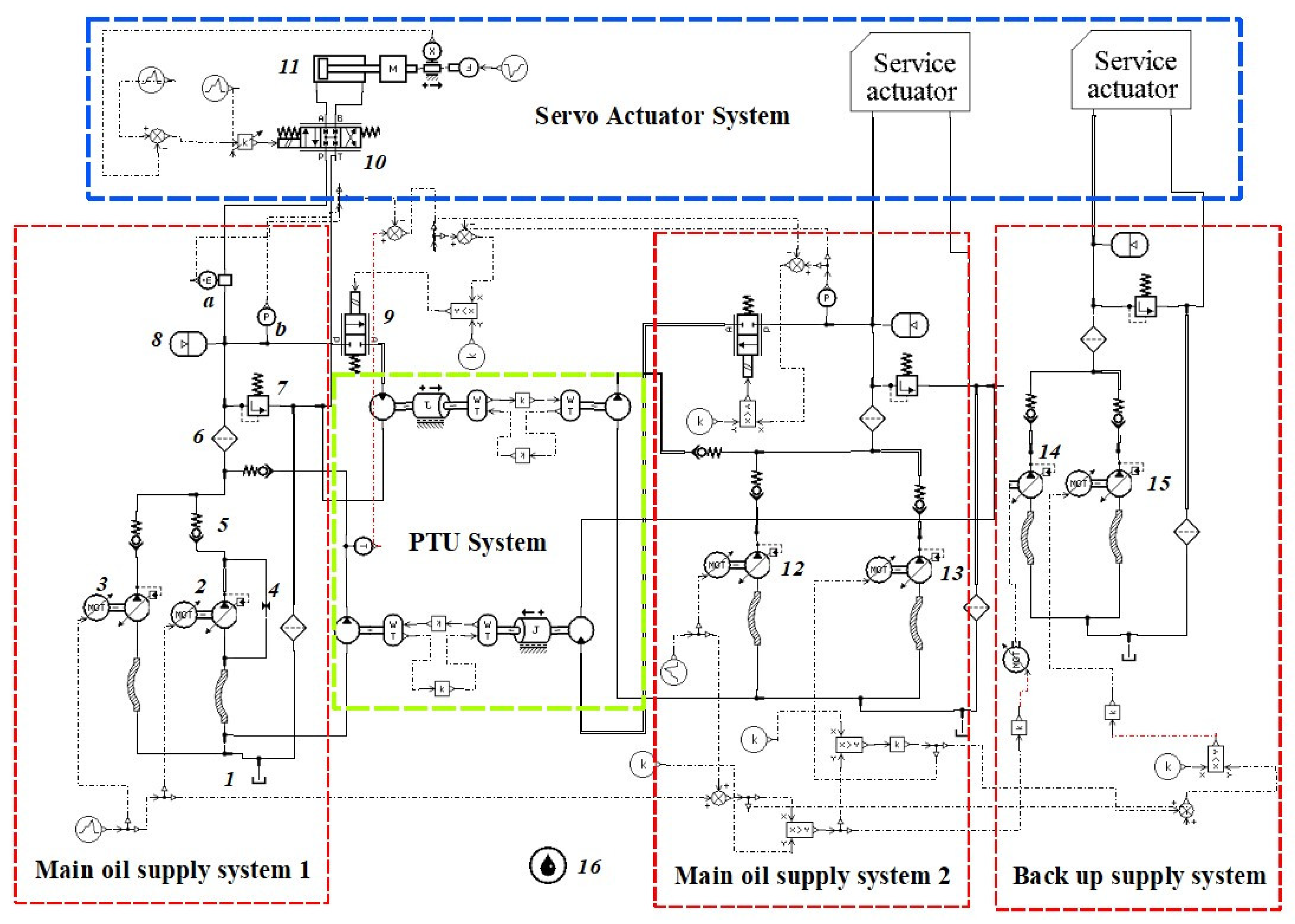
To highlight the research focus, this paper describes the study of the section from the oil tank to the actuation system without the driven part or the transmission part. The normal operation of the system means that the input signal can be transformed into a stable operation of the control surfaces. In general, an aircraft hydraulic system can be divided into two parts, namely, the servo-actuation systems and the oil supply systems. They are the core components of an aircraft hydraulic system. The aircraft hydraulic system in Figure 1 can be established by AMESIM. The AMESIM model built in this paper is shown in Figure 2.
In the AMESIM aircraft hydraulic system, being the same as in Figure 1, the oil supply system is composed of three relatively independent systems: a main oil supply system 1, a main oil supply system 2, and a back-up oil supply system.
The main oil supply system 1 is powered by a left engine drive pump (EDP,2), and an electrical motor pump (EMP,3). The main oil supply system 2 is powered by a right EDP (13) and an EMP (12). The back-up oil supply system is powered by an EMP (14) in normal state, and a ram air turbine (RAT,15) in case of the state when the left and right engines have both failed.
In the servo-actuator system which is in the blue dotted frame, the actuator (11) is used to provide mechanical energy for different oil users of the aircraft, such as the landing gear, wing flap, aileron, flipper, and rudder. The actuator control value (10) is used to control the actuator’s working time and oil pressure.
The green dotted frame between the main oil supply system 1 and the main oil supply system 2 is a two-way power transfer unit (PTU) system. In normal time, the PTU system will not work. When the pressure of one oil supply system is reduced to a low level, the PTU system will work. It transfers oil from the high-pressure side to the low-pressure side, and makes the low-pressure side return to a normal state.

2.2. Normal State and Fault State

In the AMESIM aircraft hydraulic system, one normal state and five kinds of fault states are considered in this paper.
When the hydraulic system is in operation in a normal state, the EDP (2) works at a constant speed of 5000 rpm, and outputs pressure of 3000 psi to the aircraft hydraulic system. The EDP (2) delivers oil flow from the oil tank (1) to the hydraulic system, first through a one-way value (5), which is to prevent the return of hydraulic oil, and then through an oil filter (6), which is to reduce the temperature of the hydraulic oil and prevent oil pollution. Finally, oil is delivered one way to a relief valve (7), which is used to prevent the system pressure from being too high; when the system pressure is over 3400 psi, the relief value will open and reduce the system pressure. The other way is to the actuation system. A bladder accumulator (8) ensures system pressure stability when there are sudden changes in the flow demands.
The five fault states are pump inner leakage (2), filter block (6), relief value spring failure (7), actuator inner leakage (11), and oil pollution (16). In order to improve the accuracy of fault diagnosis in the hydraulic system, eight different sensors are used in this paper. Each state has 8 kinds of different signals, including the pressure in three different places (pump, filter, and actuator), the flowrate in three different places (pump, filter, and actuator), the displacement of the actuator, and the velocity of the actuator.

2.3. Data Collection

The data of six states are simulated in the AMESIM hydraulic system. Taking the aircraft hydraulic system as the research object, eight channels signals of six different states are collected in this section. The main parameters of the AMESIM simulation model are given in Table 1. These parameters are used when the hydraulic system is in a normal state.
The fault states are built according to the normal state with consideration of the five relative values, including pump leakage (PL), filter blockage (FB), relief valve spring failure (RF), actuator inner leakage (AIL), and oil pollution (OP). By changing the five different values, the five fault states can be simulated in the AMESIM hydraulic system. The fault state parameters are listed in Table 2.
The simulation model is built when the system is stable. This simulation uses the main oil supply system 1 and the servo-actuator system to simulate the aircraft hydraulic system. When the system is working normally, it will be considered as the normal state.
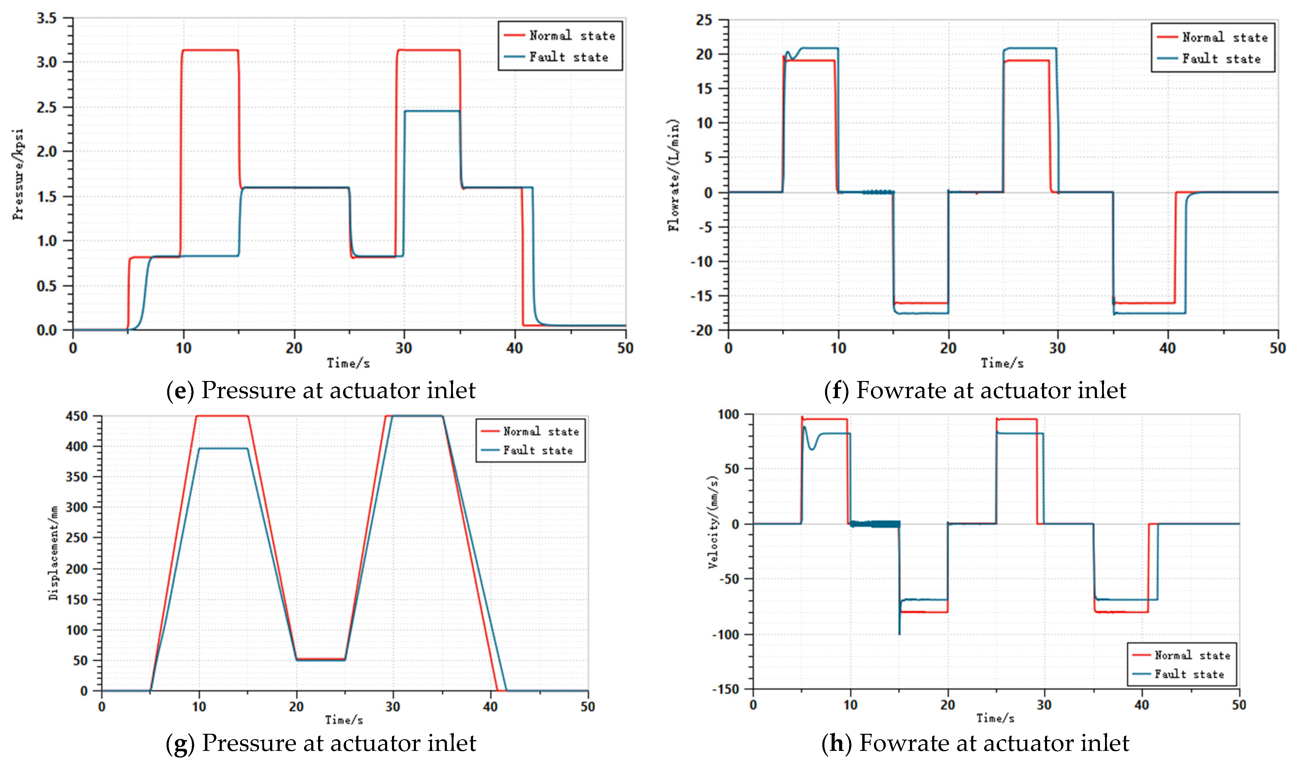
The total simulation time is 50 s, including 0–5 s during which the actuator is closed, 5–10 s during which the actuator is opened and moves left, 10–15 s during which the actuator is closed, 15–20 s during which the actuator is opened and moves right, and 20–25 s during which the actuator is closed, and then it returns to this cycle again after this simulation has ended. The sample rate is 100 hz; in each simulation, a sample of 5000 number of time point will be collected. The simulation results are shown in Figure 3. This simulation result is a comparison between the normal state and the air pollution state in eight different channel signals. Here, the oil pollution value is 0.1% in the normal state and 15% in the fault state. Due to the length of the article, the other fault state simulation results will not be presented.
After the simulations, six different kinds of data can be collected. There are eight signals that can be collected in each state, as shown in Figure 3. These include the pressure signal at the hydraulic pump outlet (Pp); the flowrate signal at the hydraulic pump outlet (Qp); the pressure signal (Pf) and the flowrate signal (Qf) at the oil filter exit position; the pressure signal (Pa) and the flowrate signal (Qa) of the actuator inlet; and the velocity signal(Va) and the displacement signal (Da) of the actuator. All the signals are shown in Table 3.

3. The EMD-LSTM Method

3.1. EMD and PCA Method

After the six states’ signals have been collected, EMD decomposition needs to be performed on each signal. The process of EMD is to decompose the original input signal into multiple IMFs. These IMFs contain different feathers in each frequency in the input signal. During the decomposition of EMD, there is no limitation on the signals of these inputs, and it does not require these input signals to be linear or smooth signals. Therefore, when dealing with the fault signals of a real-world hydraulic system with different noises, this method will have a good effect. At present, there are many research studies which applied EMD to fault diagnosis [29,30,31,32]. However, there is a lack of research on the overall multi-faults comprehensive diagnosis of an aircraft hydraulic system.
The general process of the EMD method is as follows: If x(t) is the original signal to be processed by the EMD, first, we seek all the local maximum values and local minimum values of the signal x(t). Then, we use the three-time strip curve interpolation methods and connect all the local maximum points and all the local minimum points to obtain the maximum envelope curve emax(t) and the minimum envelope curve emin(t); all data points in signal x(t) are wrapped between these two curves. We calculate the average value of the emax(t) and emin(t), and mark it as e(t). Then, we subtract the e(t) from the original signal x(t), and obtain a new signal x1(t) =x(t)–e(t). At this time, we test whether x1(t) meets the two conditions of the IMFs: 1. in the decomposed signal, the equivalent points are equal to zero or equal to one, and 2. the signal is about the local symmetry of timeline. If it is satisfied, it is recorded as IMF1 (t) = x1(t). If it is not satisfied, we use x1(t) as the original signal and repeat the above operation.
After that, IMF1(t) is separated from x(t), and we obtain a residual signal r1(t), r1(t) = x(t) -IMF1(t). Then, we use r1(t) as a new original signal to repeat the above operation. After N times, the signal can obtain N components of the IMFs, which can be expressed as follows:
r 1 t = x t I M F 1 t r 2 t = r 1 t I M F 2 t r n t = r n 1 t I M F n t
The signals after EMD decomposition are shown in Figure 4. The aircraft hydraulic oil filter blockage state is selected to the EMD. We choose three channel signals, and they are Qa, Pp, Da. The horizontal coordinates are the number of sampling time points, and the frequency is 100 Hz. The unit of each point is 0.01 s. The first subfigure is the original signal, the last subfigure is the residual r component, and the other subfigures are the IMFs, as shown in Figure 4.
The oil filter blockage (FB) state is simulated. The EMD of Qa obtains 18 IMFs, the EMD of Pp obtains 19 IMFs, and the EMD of Da obtains 12 IMFs. From Figure 4, different IMFs can reflect the characteristics of the original signal to a certain extent. Each original signal can obtain a set of feature vectors after the EMD, and the EMD results can be marked as Fn = [IMF1, IMF2, … IMFK, r], with k meaning the total number of IMFs after the EMD, and r meaning the residual after the EMD. From the three sets of EMD signals in the figures, the types of information containing and expressing are different, so the total number of IMFs are not consistent. The IMFs after the EMD enriches the input features of the LSTM networks. However, it is inevitable that there are redundancy or repetition of information, and the input dimensions of the LSTM are not the same. Therefore, the PCA method needs to be applied to reduce the dimension of the input IMFs.
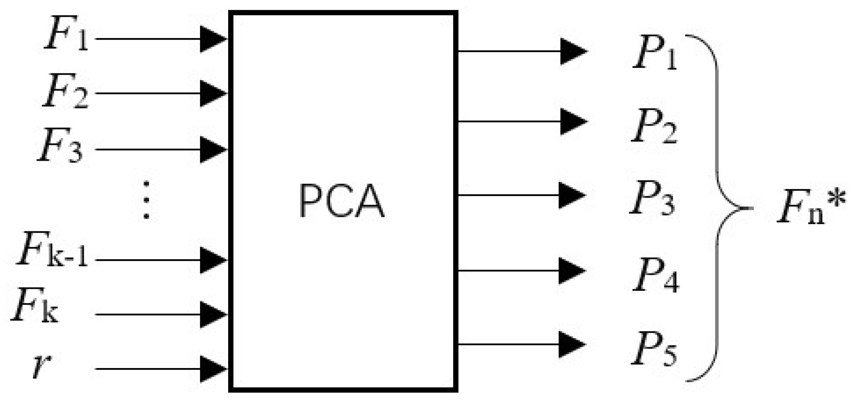
Principal component analysis (PCA) is a statistical method for the main component of a signal, and converts a set of variables that may exist into a set of linear irrelevant variables through orthogonal transformation. This set of variables is called the main ingredient. The PCA method was proposed by Karl Pearson [33]. Presently, it has been widely used in many fields, such as mode recognition, signal processing, signal compression, and fault diagnosis [34,35,36]. The PCA method can ensure that the main characteristics of a signal are not lacking and realize the simplification of data; this can greatly reduce the amount of data that requires subsequent processing. Therefore, the training and calculation time of the LSTM networks can be reduced, and the testing speed becomes faster. This process is shown in Figure 5.
Considering that the number of feature vectors are different, we ensure that the error between the real data after the dimension and the data before the dimension is less than 0.05, that is to keep the information more than 95% of the original features. The number of all Fn in this simulation is chosen as 5 IMFs. If the IMFs are higher than 5 for PCA reduction, the process is shown in Figure 5.
After the EMD and PCA, the extraction feature vector can be expressed as Fn* = [F1, F2, F3, F4, F5]. After normalization, the feature vectors are as the inputs of the LSTM networks. The total number of the inputs in the LSTM networks are 40 sets of special feather vectors. Therefore, each test or train state data set has 40 characteristic vectors.

3.2. Three Inner Structure of LSTM Networks

Long short-term memory (LSTM) neural network is a deformation of recurrent neural network (RNN). The internal structure of a RNN is a circular structure, and it can retain a certain degree of time information. Theoretically, the neurons located at the time point of ti pass their internal information to the neuron ti+1 of the next time point. In this way, the input information and the output information at the neuron of time point ti can map the effect of all the previous time points, and form a feedback structure similar to a ring. However, in an actual application of a RNN, when the distance between ti+m and ti is too large, there may be a problem that ti cannot map the input and output characteristics of the time point ti+m. This situation is called the gradient disappearance in the RNN, or long-term dependence. This problem is solved by the LSTM network algorithm proposed by Hochreiter [37]. The LSTM network adopts its unique internal three gate units structure, and through the structure of the three gate units, it can control the transmission rate in the historical information dissemination in the RNN. The information is sent into the three different gate units according to the important degree, so it solves the gradient explosion of the long distance. The mathematical expression of the LSTM model can be written as follows:
f t = σ W f · x t , h t 1 + b f i t = σ W i · x t , h t 1 + b i o t = σ W o · x t , h t 1 + b o c t ˜ = tan h W c · x t , h t 1 + b c c t = f t c t 1 + i t c t ˜ h t = o t tan h c t
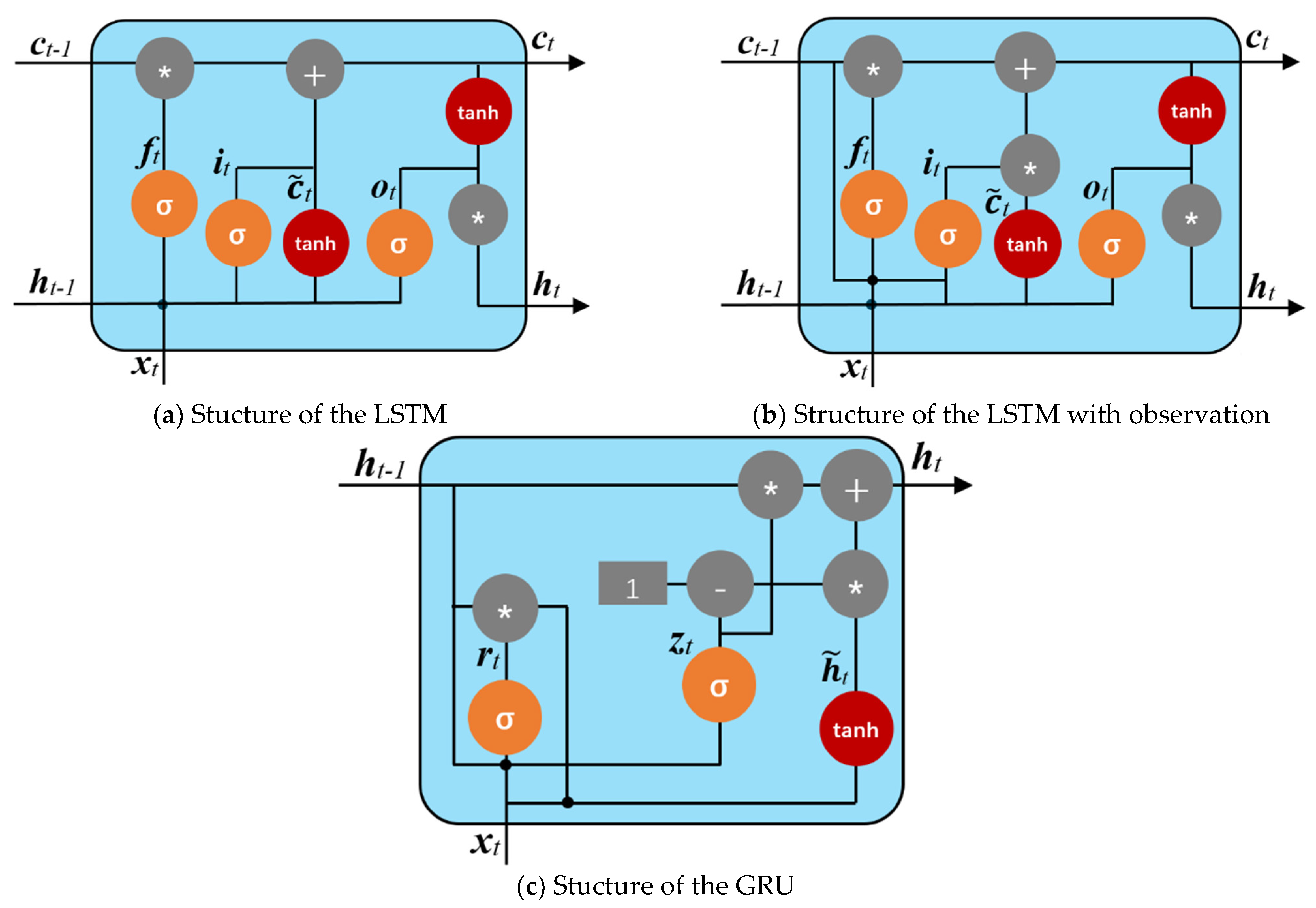
In Formula (2), t is the time point, xt is the input of the LSTM network, and ht is the output of the hidden layer in the network. ct is called the unit state, and it is a unique structure in the LSTM network. ct is used to preserve information, forget information, or control the flow of information by passing the information to subsequent neuron cells. The first three formulas are the gate unit structure, namely forgotten gate ft, input gate it, and output gate ot. These three gate structures assist ct to delete or add information, and limit the output range between 0 and 1 by the Sigmoid layer. When the output is 0, it means that the information is abandoned. When the output is 1, it means that the information is all recorded. σ is the active function, W is the weighted value of the network, and b is the offset of the network. These two parameters will be optimized during the network training. The symbols “.” and “*” here represent the matrix multiplication and the point multiplication between the same dimension matrix. The structure of the LSTM is shown in Figure 6a.
In order to choose the best internal structure of the LSTM, the other two different internal structures of LSTM networks are considered in this paper. LSTM also has a variety of internal structural design methods, and by changing the internal structure of the network, it can change its effect on fault classification. Among the current commonly used methods, there is a structure called LSTM with observation holes. This network structure is set up inside the network by changing the settings of the three units, and adds a part of the ct-1 observation for each unit status at the previous time point. The structure of LSTM with observation is shown in Figure 6b. Compared to the traditional LSTM network structure, this structure is more complicated, and the mathematical expression can be written as follows:
f t = σ W f · x t , h t 1 , c t 1 + b f i t = σ W i · x t , h t 1 , c t 1 + b i o t = σ W o · x t , h t 1 , c t + b o c t ˜ = tan h W c · x t , h t 1 + b c c t = f t c t 1 + i t c t ˜ h t = o t tan h c t
In addition, there is another structure of LSTM which is called gated recurrent unit (GRU), that is applied in the field of fault diagnosis and has a relatively novel structure. Compared to the traditional LSTM, it simplifies the internal structure, but the accuracy of classification of a GRU can achieve considerable or better results. In addition, it is easier to train in comparison, and it can largely improve training efficiency. Therefore, GRU is more inclined to be used in the field of fault diagnosis. It simplifies the internal structure of the standard LSTM, integrates the forgotten gate and the input gate as a new structure called update gate zt, and introduces rt as the reset gate. The structure of the GRU is shown in Figure 6c. Its expression can be written as follows:
z t = σ W z · x t , h t 1 + b z r t = σ W r · x t , h t 1 + b r h t ˜ = tanh W h · x t , r t h t 1 + b h h t = z t h t 1 + 1 z t h t ˜
Figure 6 shows the structures of the three different kinds of LSTM neural networks.

3.3. The LSTM Network Structure Design

The input layer of the LSTM is 40 IMFs. In the LSTM layer, each internal unit is spliced in order, and at each time, on the long step, we perform a state of states at a hidden layer and data update; this process is called a unit time step process.
The characteristic input at the current moment and the implicit unit status of the previous moment are used as the input of the hidden unit in the next step to update the state. The mathematical expressions of the three different LSTM methods are shown in Formulas (2)–(4). After that, the output of the LSTM layer is connected with a fully connected layer (FC 1), and this fully connected layer uses the ReLU activation function to restrict the output above 0. Then, the output of the FC 1 is connected to a second fully connected layers (FC 2). This layer with the SoftMax function layer forms the output layer. The output is a possible state for the samples, and it represents five types of fault states and a normal state. The structure is shown in the Figure 7.
The input layer is 40 characteristic data samples after preprocessing. The input neurons are 40, each data column length is 5000, the sampling frequency is 100 Hz, and the number of neurons in the LSTM layer is 12. The number of neurons on the first fully connected layer is 12. The number of neurons on the second fully connected layer is 6. The number of neurons in the Softmax layer is also 6, which is the six different states’ output.
The three LSTM models in this article are built based on the TensorFlow2.0 GPU framework, computer matching: Intel (R) Core (TM) i5-12400F CPU @ 4. 40 GHz + NVIDIA GEFORCE RTX 2070 super 8 GB. The batch size is set to 800, and the maximum number of iterations is 200 times. During the model training, the loss of the task is calculated with cross-entropy loss, and it is used as the total loss of the model. Due to the fast convergence speed of the Adam optimizer and less memory demand, it can reduce the performance of the device. Therefore, the Adam algorithm is chosen as the optimizer and the learning rate is set to 0.001 to optimize the model. The proportion of the task is adjusted to the optimal training effect of the tasks. The main parameters of the network are shown in Table 4.
Table 4 lists the optimal values for the network parameters, where lr is the learning rate and the batch size refers to the number of batch samples. The dropout rate refers to the random resetting of the neuron output to zero with a certain probability during training, which can help reduce over-fitting. The optimal parameter is obtained based on the actual situation of the aircraft hydraulic system and multiple experiments.

3.4. EMD-LSTM Method for the Aircraft Hydraulic System

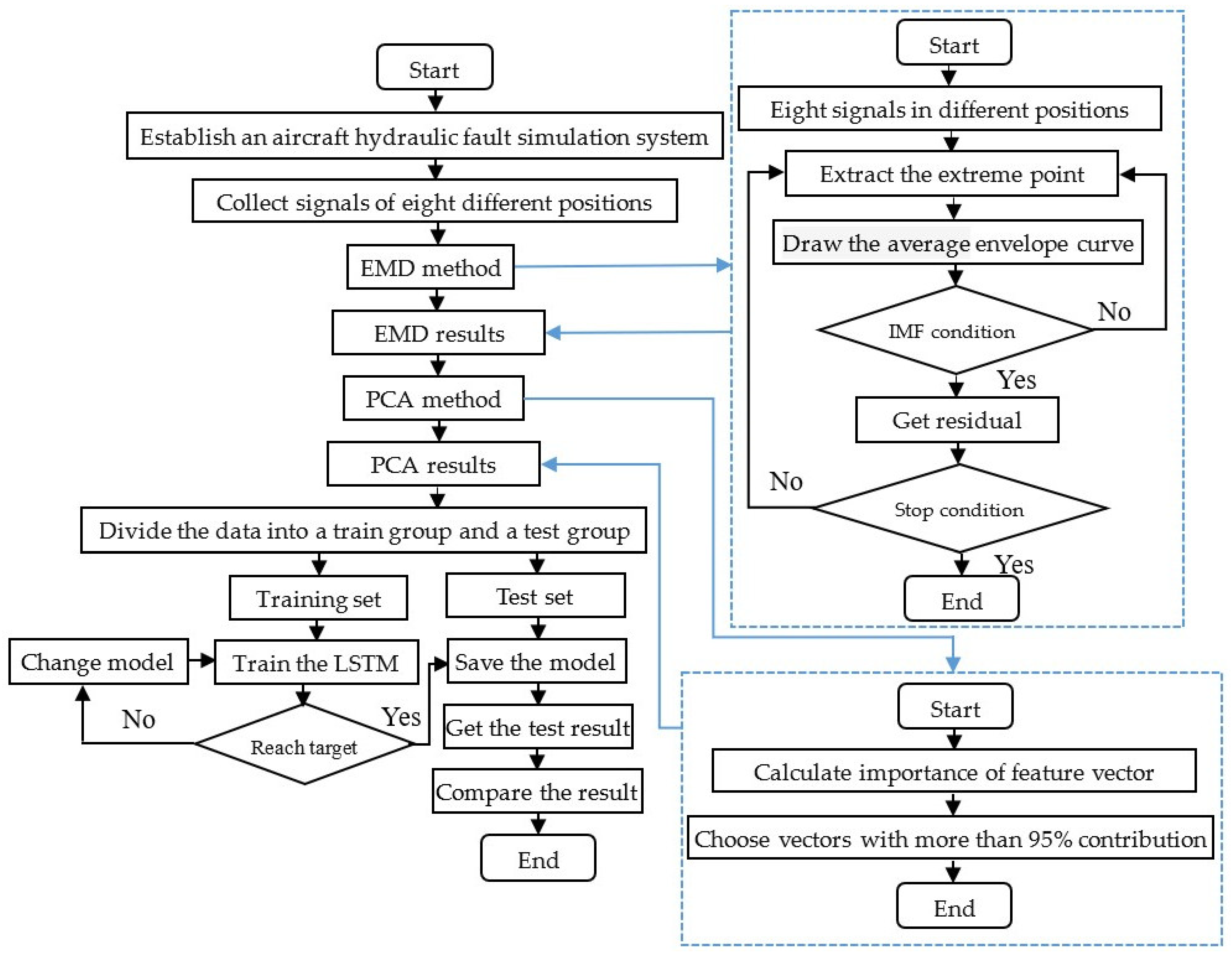
This paper focuses on the fault diagnosis of an aircraft hydraulic system in a noisy environment, and a fault diagnosticmethod based on EMD-LSTM is proposed in this article. The collection data include the six different states of signal data obtained by the AMESIM simulation in Section 2. Eight sensors are used for each state to collect data, including three data sets of oil pressure (pump, filter, and actuator), three data sets of oil flow rate (pump, filter, and actuator), a displacement data set, and a velocity data set. First, the EMD method is used to decompose the collected eight-channel aircraft hydraulic system fault data to obtain the data characteristics of the IMFs. Then, the PCA method is used to reduce the dimensions of the IMFs. On the premise of ensuring the effectiveness of the data, the main feature component is extracted from the different decomposition results of multiple groups to reduce the data processing amount for subsequent fault diagnosis, and to improve the efficiency and the speed of fault diagnosis. Finally, the IMFs with high correlations after dimension reduction are used as the training and test sets to train and test the three LSTM networks with different internal structures. The flow chart of the EMD-LSTM method is shown in Figure 8.

4. The Simulation Results of the EMD-LSTM Method

4.1. Data Collection and Feature Extraction

The data samples used for training and testing of the LSTM are obtained through simulation of the aircraft hydraulic system model in the second section. The six categories of states contain a normal state and five types of failure are simulated. Among them, 1000 experimental samples are collected, of which 800 samples are randomly selected as the training sets and 200 samples are selectd as the testing sets.
In an environment with higher noise, featured information is often drowned in noise. It is difficult to use the timing signal training network for fault diagnosis. Therefore, signal preprocessing is considered in this paper, and the feature information is obtained before the LSTM fault diagnosis. In this paper, the data are preprocessed using the EMD method to obtain different IMFs. Then, the PCA method is used to reduce the dimension of the IMFs obtained. There are 5 IMFs in each channel, and we transform the network training data set from 8 channels to 40 channel sample sets. The length of each data sample is 5000 sampling points, and the sampling frequency is 100 Hz. These characteristics of different IMFs can reflect the characteristics of different states of hydraulic systems. The number of samples in different types is specifically shown in Table 5.

4.2. The Fault Diagnostic Results in the Comparison of Three EMD-LSTM Methods

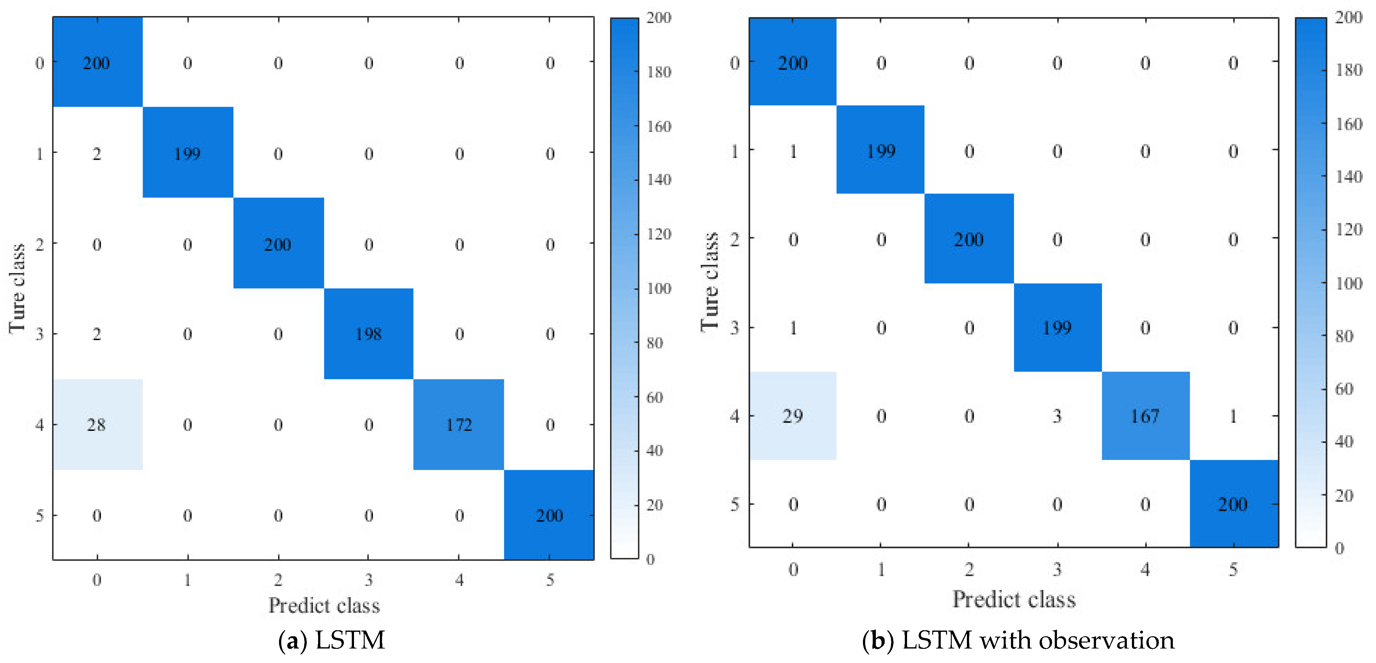
In the simulation experiment, the LSTM neural networks with three different internal structures are used to perform fault diagnosis of the hydraulic system. The accuracy, testing time, and hardware size are considered in the three LSTM fault diagnostic methods to compare the fault diagnostic effect. In order to compare the impact of structure on the LSTM network, the other parameters of the network are set to stay consistent, and only the internal structure in the LSTM layer is changed. The confusion matrix of the three different structures of LSTM network diagnosis is shown in Figure 9.
From Figure 9, the accuracy of the three LSTM methods are high, and the accuracy of all methods reaches more than 97%, Therefore, these three methods are feasible methods for the fault diagnosis of aircraft hydraulic systems. Relatively, the accuracy of the GRU method is highest and reaches more than 98%.
From a single failure, the accuracy of class 4 is lower than the other classes. Class 4 is the oil pollution state of the aircraft hydraulic system. From the figures, the accuracy of the LSTM method is 86%, the accuracy of the LSTM with observation is 83.5%, the accuracy of the GRU method is 90%, and almost all of the oil pollution states predict the normal state. This is because when oil pollution is under a low level, it has a small impact on the entire aircraft hydraulic system. Therefore, inaccurate situations appear in the fault diagnosis. In general, low oil pollution degree does not have a great impact on the aircraft hydraulic system, and can reduce oil pollution by regular replacement of hydraulic oil filters. Specific overall accuracy, system training time, and hardware resource consumption are shown in Table 6.
The simulation results show that the accuracy of the three LSTM methods is higher than 97%, and the GRU method has the highest accuracy at 98.25%. These simulation results show the method of EMD-LSTM is the best method for fault diagnosis of an aircraft hydraulic system. In the comparison of the testing time and hardware resource consumption, it can be seen that the testing time is all relatively short. Basically, the operation time can be counted. In terms of hardware resource consumption, the GRU method has simplified the input door and output door, and due to the simple internal structures, the GRU is more advantageous than the LSTM and the LSTM with observation in terms of hardware resource consumption.
Comparing Figure 9 and Table 6, the internal structure of the GRU as the LSTM network is more suitable for the fault diagnosis of aircraft hydraulic systems, and the research on anti-noise performance will be based on EMD-GRU.

4.3. EMD-GRU Network Structure and Parameter Optimization

To optimization the performance of the EMD-GRU model, the GRU network structure, the learning rate, and the batch size are chosen to test the EMD-GRU method.
(1) The structure of the method will affect the fault diagnostic results. In order to prove the advantages of the EMD-GRU method in this article, three comparison classes of different structures are selected to compare with the EMD-GRU method.
The first class does not use the EMD method or the PCA method, and directly uses the 8-channel signals to train and test the GRU networks. The second class does not use the PCA method and uses all the IMFs to train and test the GRU networks. The third class uses the EMD method and PCA method, but the GRU networks are separated to eight different GRU networks, and each network uses five IMFs to train and test the GRU. At last, the eight GRU networks are used to obtain eight fault diagnostic results, and the eight fault diagnostic results are used to vote for the final result of this method.
To test the effect of structure on the fault diagnostic results, the parameters in the different structures are the same. Each structure is simulated 10 times to obtain the average accuracy and testing time. The simulation results are shown in Table 7.
From the simulation results, it can be seen, in the class of the structure that does not use EMD for feature extraction, the accuracy decreases significantly. The accuracy of the GRU network structure reaches 93.16%. From class 2, which is the structure that does not use PCA dimension reduction, the accuracy rate also decreases, but the decline is not obvious, with only about 2% decrease. Therefore, the EMD decomposition is effective for the extraction of features. The IMFs have not been reduced by PCA, so data redundancy and duplication lead to an increase in testing time, because the input in each group of test groups tested increases significantly. According to the analysis of 3.1, IMFs increase from 5 to 15–19. Therefore, PCA dimension reduction can also effectively increase the accuracy of GRU fault diagnosis. From class 3, the EMD and PCA methods are used in this class. However, during the training process of the GRU, the features of 40 IMFs are not processed into the same GRU networks. Instead, eight GRU networks with homogeneous structures are used for separate training, then the voting decision is used to classify the states. In this process, there is a problem with the integrity of the information; as a result, the accuracy rate also decreases, but it is still higher than the accuracy of the solution that does not adopt EMD. However, the size of the model under this situation is the largest, and it is not suitable for application in an aircraft hydraulic system because multiple network operations at the same time take up more hardware equipment resources, and it does not bring a significant increase in detection speed or a significant improvement in accuracy.
According to the content of the above table, it can be seen that the EMD method feature extraction is used, and the PCA method is used to reduce the dimension. Finally, the 40 IMFs is introduced into the same GRU network for training. In this way, the accuracy of the EMD-GRU is the highest. The accuracy of the internal structure of the GRU can reach 98.25%, and hardware resource consumption is relatively small; this structure of GRU is the best structure for aircraft hydraulic system fault diagnosis.
(2) The learning rate and the batch size. In addition to the structure of the model, the GRU internal parameters’ setting will also affect the effectiveness of the fault diagnosis. The learning rate and the batch size have a greater impact on the GRU networks. We analyze the effects of these two parameters and select the best parameters.
To prevent the simulation from being affected by other factors, a single variable is used to simulate, and each training only changes the value of one parameter, while all other parameter values are fixed. The input signals are 40 characteristic IMFs, and the internal structure also uses the GRU structure.
The learning rate has a great impact on the reverse update speed of the GRU network. If the learning rate is too large, it will cause the network parameters to swing back on both sides of the optimal solution and it will be difficult to obtain the optimal solution. If the learning rate is too small, it will cause the gradient to drop too much and cause the gradient to disappear. Therefore, the GRU can increase learning rate attenuation to prevent the gradient from disappearing.
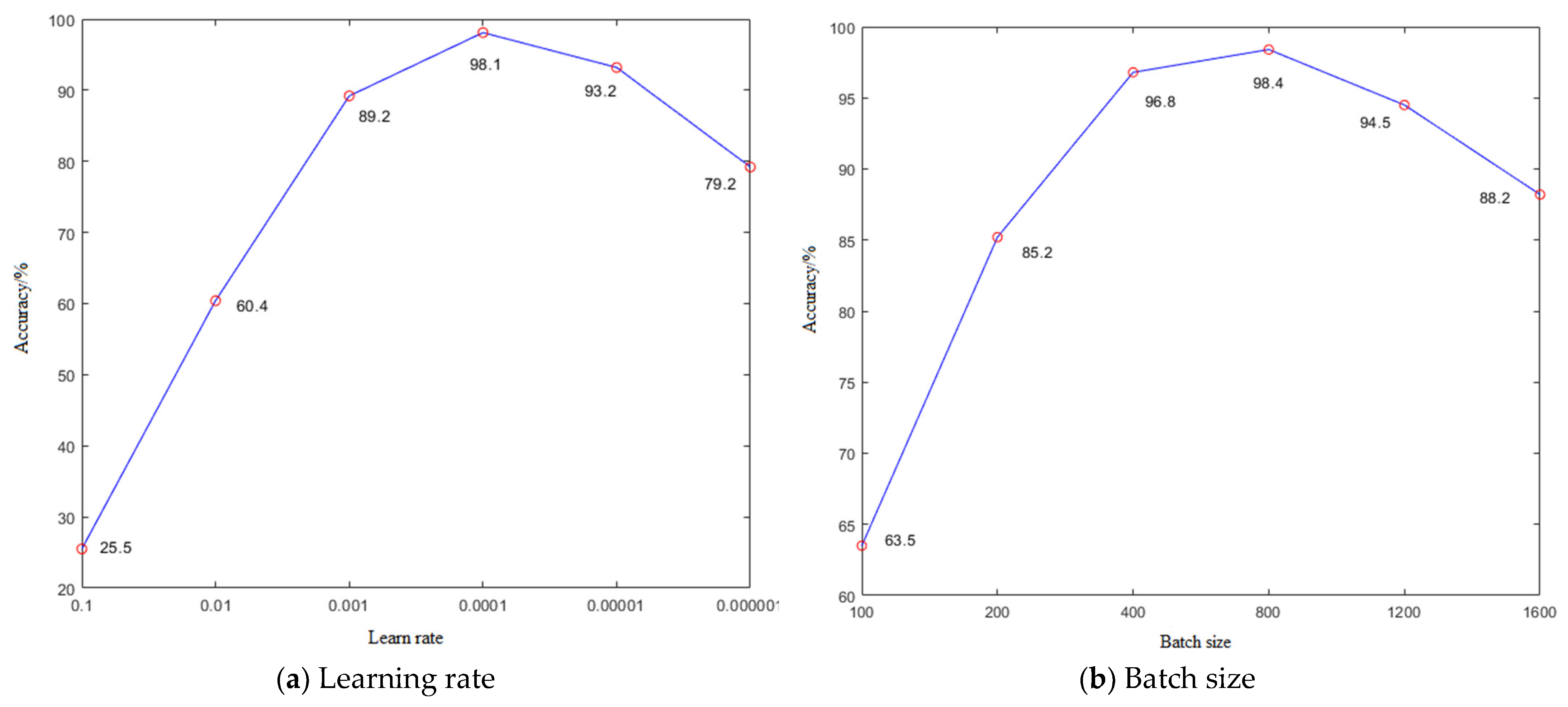
The batch size is a method of updating the network parameters to divide the input sample in the network training. Avoid the input of a single sample that causes the optimal problem. Increasing the number of iterations can increase the accuracy of the network. However, the network training time and fault detection time will be extended. The simulation results are shown in Figure 10 and Table 8.
As can be seen from Figure 10a, the learning rate can affect the accuracy of the fault diagnostic results of the GRU network. When the learning rate is relatively low, the learning speed of the network is fast, and as a result, the accuracy of the fault diagnosis is relatively low. When the learning rate is relatively high, the amount of data from learning is relatively small, and the GRU network is difficult to make effective fault diagnosis. In the diagnosis of the aircraft hydraulic system, when the learning rate is 0.001, 0.0001, and 0.00001, the accuracy of the failure diagnosis of the GRU network is relatively high. The accuracy all reaches more than 90%. From Table 8, when the learning rate is 0.00001, the training time is longer. Comparing Table 8 and Figure 10, when the learning rate is 0.0001, the training time is shorter and the accuracy is highest. Therefore, 0.001 the best learning rate of GRU networks.
From Figure 10b, different batch sizes will also affect the accuracy of the fault diagnosis. Compared to the impact of the learning rate, the impact of the batch size is not particularly obvious. It can be seen from the figure that when the amount of the batch size is 400, 800, and 1200, the accuracy of the GRU can reach above 95%. Among them, the accuracy rate is up to 98% when the batch size is 800.
From Table 8, when the batch size is small, the training time will be relatively long. This is because the total number of data loads in each training cycle is consistent and each input batch size is small; therefore, it is necessary to enter a large number of samples. In most cases, the reduction of the batch size can increase the accuracy of the fault diagnosis. For example, the accuracy rate should be increased when the batch size is changed from 800 to 200. However, in the aircraft hydraulic system fault diagnosis, when the batch size is lower, the accuracy of the fault diagnostic results cannot be improved; instead, there will be a decline. It is because, in the failure diagnosis of the aircraft hydraulic system, the characteristics of the signals of each state often do not appear in a short time. In a signal of 200 sample points, the signal features of different states are extremely similar, so the batch size is lower and the accuracy of the fault diagnosis is lower too.
Comparing Figure 10b and Table 8, when the batch size of the GRU network is set to 800, the training time is relatively short and the accuracy of the fault diagnosis of the GRU network is higher. The batch size is set to 800 for fault diagnosis in the EMD-GRU method.
Therefore, through the three groups of the simulation results, the optimized structure is adding the EMD and PCA methods in the network structure, and using 40 IMFs as the input to train the GRU networks. The optimized parameters of the GRU are when the learning rate is set to 0.0001 and the batch size is set to 800.

4.4. Noise Addition and EMD-GRU Fault Diagnosis under Different Noise Environments

In this article, Gaussian white noise is used to add to the 8-channel signals in the aircraft hydraulic system. Gaussian white noise refers to the probability distribution that conforms to Gaussian distribution, and the power spectrum density meets the noise of uniform distribution. It is an ideal model for analyzing channels with sexual noise. The signal-to-noise ratio (SNR) is a common indicator of noise in a signal. It also adds to different degrees of noise measurement. If the noise of m dB is added, the calculation is shown in the following formula:
m = 10 l o g 10 P s P n  
In the Formula (5), Pn is the Gaussian white noise power of m dB and Ps is the power of the original signal. The power calculation of the signal is shown in Formula (6):
P = i = 1 n s i 2 N  
In Formula (6), N represents the number of data points and si means the number i data point. K times of Gaussian white noise is still Gaussian white noise; in order to generate m dB of Gaussian white noise, it can generate a set of standard normal distribution of Gaussian white noise, and take a multiplier m to generate the Gaussian white noise of m dB. Its calculations can be found through Formulas (7) and (8):
P n = i = 1 n k × n s i 2 N = k 2 × P n s  
P n = P s 10 m 10  
In Formulas (7) and (8), nsi and Pns mean the number i data point and the corresponding power of the Gaussian white noise. Then, different SNR noise is added to the eight-channel original signals.
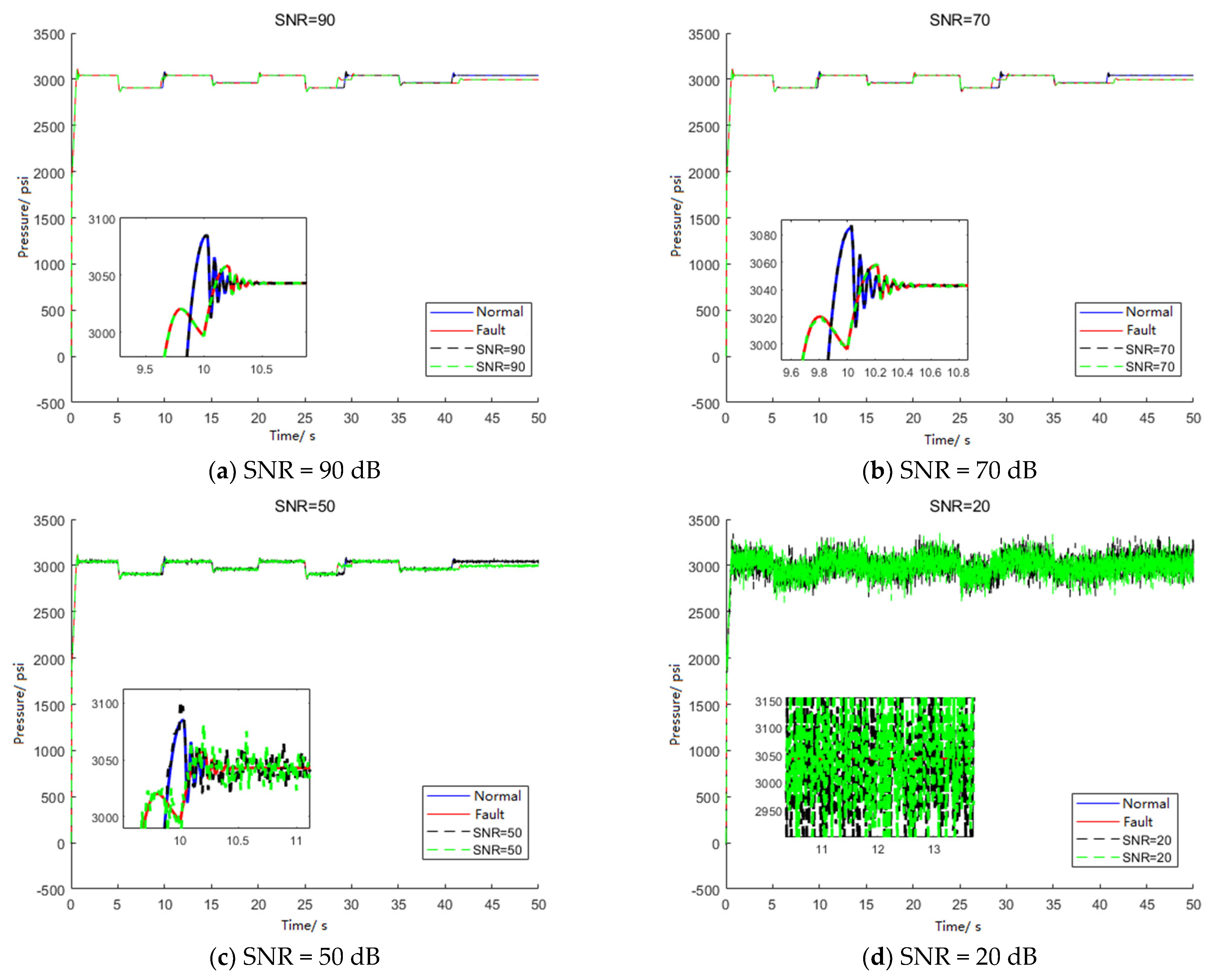
Figure 11 is a comparison figure of the original signals and the added noise signals. In Figure 11, the normal state signal and the fault state of the hydraulic oil filter blockage are selected and different SNR noises are added to them. The blue line in the figures is the pump outlet pressure signal in the normal state, and the red one is the fault state. The black dotted line adds noise of different SNR to the normal state, and the green dotted line adds noise of different SNR to the fault state. The small window in each figure is an enlarged signal to a certain time period, which can see the changes of the four state signals more clearly.
In Figure 11a,b, the environmental noise is not high, the process of the amplitude of the oil pressure can be observed clearly, and this ensures that the accuracy will not decrease significantly within this range. The pressure changes in Figure 11c have been covered by noise signals, only through amplification that the change process can be seen clearly, and, thus, the environmental noise statement is obvious. In Figure 11d, the entire signal is almost completely annihilated in the noise environment.
Then, the anti-noise performance simulation of the EMD-GRU is simulated. In the simulation experiment, all the signals collected from the AMESIM aircraft hydraulic system are added different Gaussian white noises to imitate the environmental noises in the aircraft hydraulic system in an actual working situation.
In the simulation, different SNRs are selected to add noise to simulate different SNR noise environments. The noise of the EMD-GRU method in the diagnosis of faults affects the size, and the results of the fault diagnosis are obtained in different noise environments. The SNR of the white noise in this simulation is 90 dB, 80 dB, 70 dB, 60 dB, 50 dB, 40 dB, 30 dB, and 20 dB.
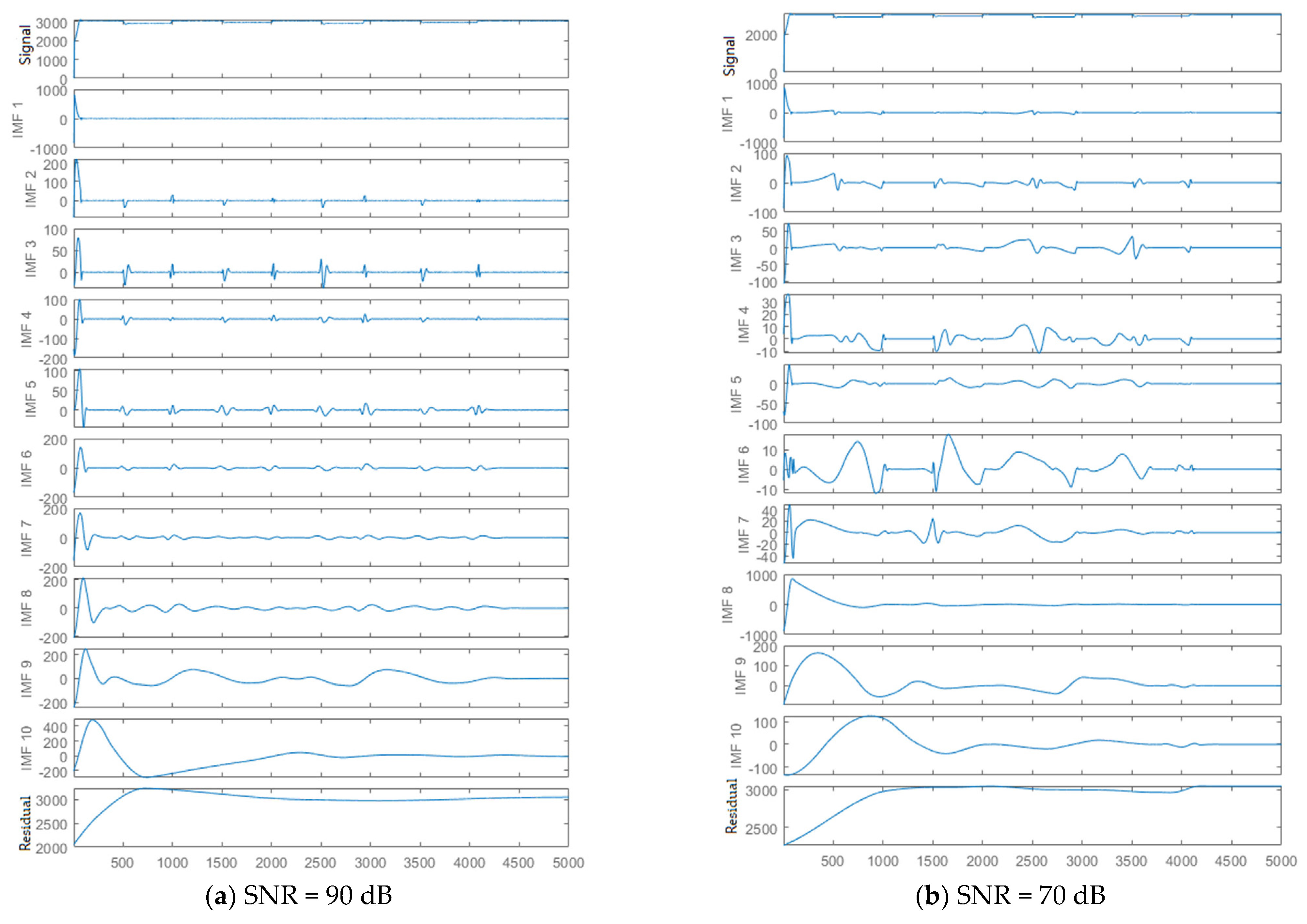
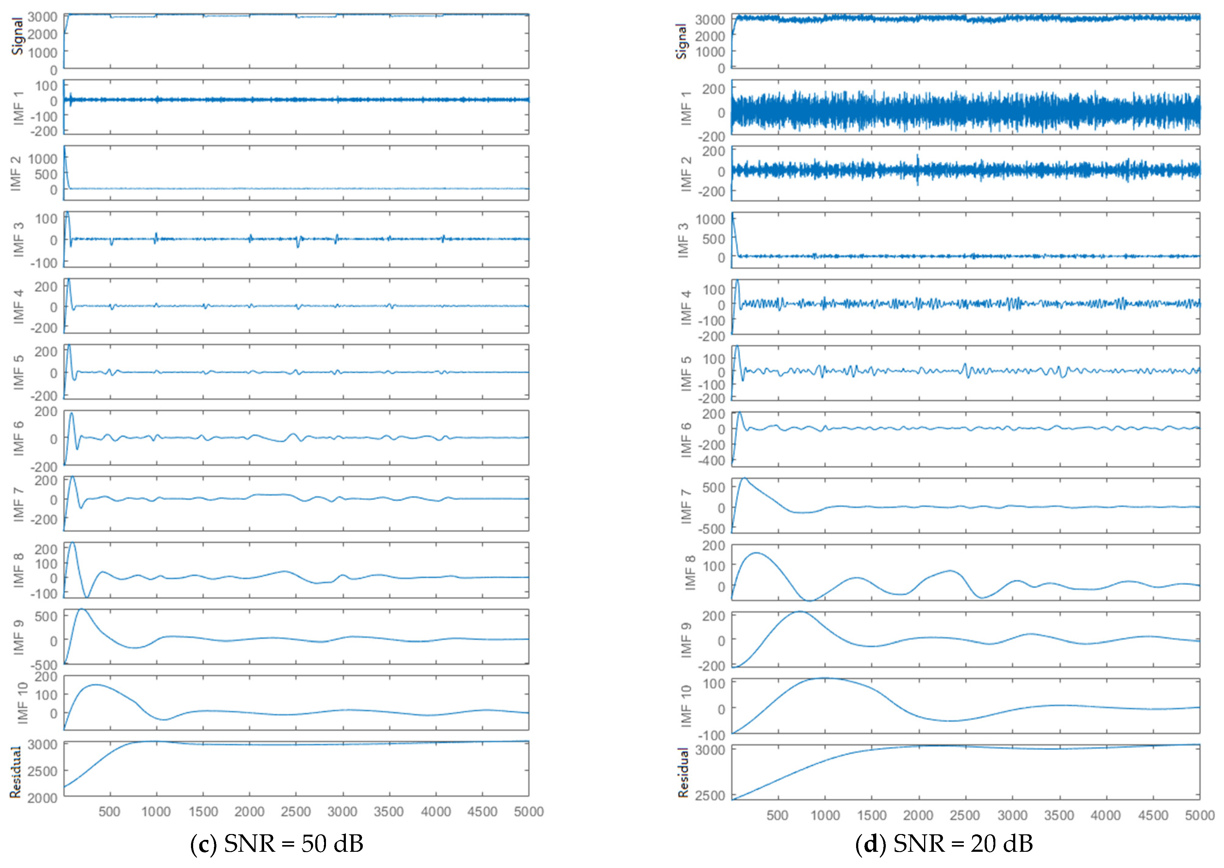
First of all, the added noise signals need to undergo EMD to obtain their characteristic components, IMFs and residual r; multiple IMFs after decomposition is shown in Figure 12. During the EMD process in the figure below, in order to calculate more conveniently, we only calculate the decomposition of 10 IMFs and then stop the EMD process. Therefore, each signal is decomposed into 10 unified IMFs and a residual r. The EMD results of the signals under different SNR noise are shown in Figure 12.
As shown in Figure 12, the label on the left is the number of the decomposed IMFs, the first subfigure is the original signal, the following 10 subfigures are IMF1~IMF10, and the last one is the residual r. The horizontal axis of the coordinate shaft is the number of time points, the sampling frequency is 100 Hz, and the corresponding time for each sampling point is 0.01 s.
From the results in the figures, the rationality and effectiveness of the EMD feature extraction are demonstrated. Because in different noise environments, the distribution rules of the input characteristics after EMD have obvious similarities, unlike the timing signals which are difficult to distinguish. The IMFs can be treated as characteristic vectors of a certain state to train the GRU neural network. Some states can even be easily identified based on a few features. On the other hand, the result of this decomposition also illustrates the necessity of using GRU as a fault state classifier. For such a complex characteristic distribution law, it is almost impossible to diagnose real-time faults by human. The GRU-based classifier proposed above can learn this inherently distribution law independently, and then make a timely judgment and assessment of the system conditions based on the input testing data.
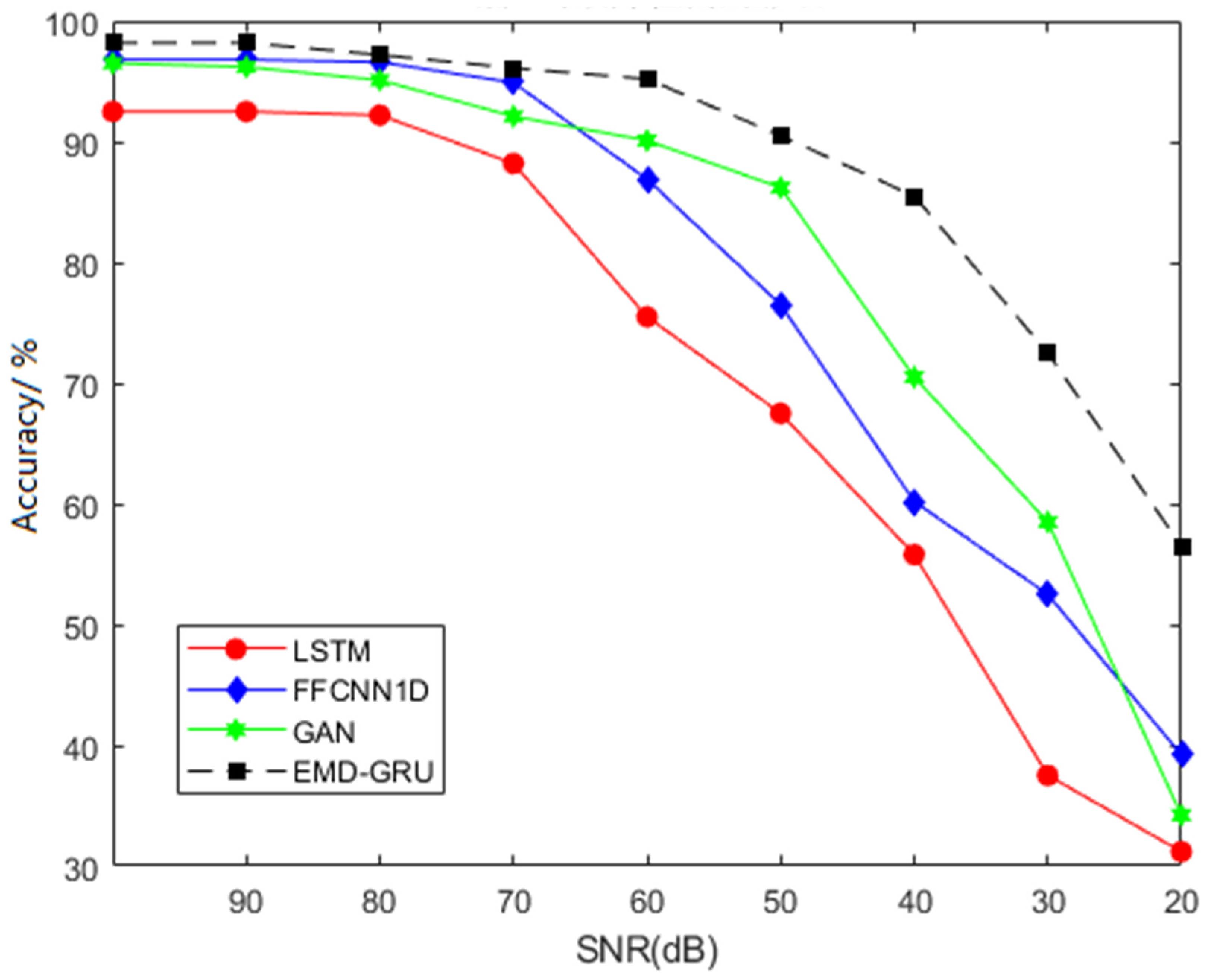
After obtaining multiple different IMFs under different noises, the five component IMFs that are related to the original signal are selected for PCA dimension reduction. Then, the GRU network is trained. The relationship between the EMD-GRU method classification results and environmental noises is shown in the Figure 13. The black dotted block in the figure represents the EMD-GRU method. In order to compare the effect of its anti-noise resistance, three methods are adopted as a comparison group to compare the noise performance of this method. This includes the blue block which represents the FFCNN1D method [38], the GAN [39] method is represented by the green stars, and the traditional LSTM network is represented by the red dots. The LSTM network structure does not use EMD or PCA dimension reduction. The comparison of the diagnostic results of these four model structures in different noise environments is shown in Figure 13.
As can be seen from the Figure 13, in the four methods, the EMD-GRU method has the best effect to resist noise. When the noise is over 70 dB, these four methods can maintain a high accuracy which is over 90%. When the noise is from 70 dB to 50 dB, the fault diagnostic accuracy of the 1DFFCNN and LSTM methods have fallen rapidly. When the noise SNR is equal to 50 dB, the accuracy rate of the 1DFFCNN is reduced to less than 80%, and the accuracy of the LSTM method drops to less than 70%. At the same time, the GAN method and the EMD-GRU method also have a better classification. The accuracy of the two methods are above 90%. When the SNR of the environment noise reaches 40 dB, the accuracy of the GAN method begins to decline rapidly, but the EMD-GRU method still has a good classification ability in this noise environment. The accuracy of its classification can reach more than 85%. When the SNR of the noise environment reaches 30 dB, the accuracy of the EMD-GRU method also begins to decline and the accuracy is near 70%, but it is still higher than the accuracy of the other three methods. When the environmental noise reaches 20 dB, the accuracy of the three comparison methods is less than 40%, and these three fault diagnostic methods can not be applied to aircraft hydraulic systems. However, the diagnostic accuracy of the EMD-GRU method remains around 60%, which has a certain diagnostic effect.
The simulation results show that the EMD-GRU method can resist strong environmental noise when the SNR is over 30 dB, and this method can still run stably in a high-noise environment. Therefore, this method is suitable for the fault diagnosis of aircraft hydraulic systems, and has a wide range of actual application potential.

4.5. Comparison between EMD-GRU Method with Various Other Fault Diagnostic Methods

In order to compare the fault diagnostic effects of the EMD-GRU method and different fault diagnostic methods in different noise environments, five common machine learning models are selected for comparative studies. These models include three traditional machine learning models, back propagation (BP), support vector machine (SVM) [40], and random forest (RF) [41], as well as two deep learning models, namely convolutional neural network (CNN) [42] and long short-term memory (LSTM) [43].
Among them, the BP neural network is an early traditional shallow neural network algorithm, and the BP network structure adopted in this article is a four-hidden layer structure. We choose the splicing fusion method to stitch the signal of the eight channels, generate an input signal with a length of 40,000 sample points, and train the BP network. The first hidden layer nodes are set to 2400, the second hidden layer nodes are set to 512, the third hidden layer nodes are set to 128, and the output layer nodes are set to 6. In addition, we use the ReLU activation function. For the structure and parameter setting of the other four methods, refer to the literature. The simulation mainly compares the diagnostic results in three different states: no-noise environment, low-noise (70 dB) environment, and high-noise (40 dB) environment. The simulation results are shown in Table 9.
The simulation results show that, in an environment without noise, the accuracy of the EMD-GRU algorithm aircraft hydraulic system fault diagnosis is the highest. Compare to the three classic machine learning algorithms, BP, SVM, and RF, the accuracy rate of the EMD-GRU method is relatively high, and the accuracy of GRU is 23.05% higher than that of SVM. Compared to the deep learning methods, the accuracy of the CNN method has the lowest accuracy, and while the LSTM does not use EMD and PCA, its accuracy rate is higher than the CNN.
In a low-noise environment (SNR = 70 dB), the accuracy of the diagnosis of each method decreases, but the decline in the deep learning methods is not obvious. In the traditional machine learning methods, the decline in the accuracy of the RF is relatively not obvious, but the BP and SVM have obvious decreases. At this time, the accuracy of the EMD-GRU is still higher than 95%, which has a good classification effect.
In a high-noise environment (SNR = 40 dB), the advantage of the method proposed in this article is obvious. The accuracy of the EMD-GRU method can still be maintained at about 90%. The accuracy of the other methods decreases significantly. The accuracy of the EMD-GRU method is 64% higher than the BP network. The accuracy of other deep learning models in a high-noise environment also drops to nearly 60%; thus, these deep learning methods can perform fault diagnosis at this time, but the results of the fault diagnosis cannot be guaranteed.
Through the above simulation results and analysis, the EMD-GRU method proposed in this article can effectively resist environmental noises and perform accurate fault diagnosis in a noisy environment. Judging from the simulation results, this method can be diagnosed stably in the case of 40 dB environmental noise, and the accuracy is near 90%. The EMD-GRU method provides an effective solution to solve the fault diagnosis of an aircraft hydraulic system in a noisy environment.

5. Conclusions

In this paper, an EMD-GUR method was proposed to deal with the fault diagnosis of an aircraft hydraulic system in different noisy environments. First, the aircraft hydraulic system was constructed by the AMESIM, and a normal state and five fault states were considered. Eight different signals of six states were collected by AMESIM simulation. Second, the EMD and PCA methods was used for preprocessing of the eight-channel signals, and five IMFs were selected as the input features for fault diagnosis in the LSTM networks. Then, three different inner structures of the LSTM networks were presented. The whole structures of the three LSTM methods were designed, and the main parameters were provided. At last, the flow chart of the EMD-LSTM fault diagnostic method for the aircraft hydraulic system was presented. Third, the fault diagnostic results of the three LSTM methods were obtained through simulation, and the simulation results show that the internal structure of the GRU as the LSTM network is more suitable for the fault diagnosis of aircraft hydraulic systems; thus, the research on anti-noise performance was based on the EMD-GRU. Fourth, the structure and the parameters of the EMD-GRU were optimized to choose the best structure and parameters for our research on fault diagnosis in different noisy environments. Fifth, Gaussian white noise with different SNRs were added to the 8-channel signals, and the simulation results of different noisy environments are presented. Then, a comparison between the EMD-GRU method with various of other fault diagnostic methods was performed using simulation, and the results show the method in this article has a better performance in a high-noise environment. In summary, the EMD-GRU method is a suitable fault diagnostic method of the aircraft hydraulic system under a noisy environment.
For the EMD-GRU method proposed in this article, the fault diagnostic accuracy can reach more than 90% in the 40 dB noise environment. However, when the noise is higher than 20 dB, the fault diagnostic accuracy cannot be guaranteed. In future work, the fault diagnostic methods of the aircraft hydraulic system in a higher-noise environment will be considered.

Author Contributions

Software, formal analysis, data curation, and writing—original draft preparation, K.S.; Writing—review and editing, and supervision, D.Z. All authors have read and agreed to the published version of the manuscript.

Funding

This research received no external funding.

Institutional Review Board Statement

Not applicable.

Informed Consent Statement

Not applicable.

Data Availability Statement

The data is in the paper.

Conflicts of Interest

The authors declare no conflict of interest.

References

  1. Reveley, M.S.; Briggs, J.L.; Evans, J.K.; Sandifer, C.E.; Jones, S.M. Causal Factors and Adverse Conditions of Aviation Accidents and Incidents Related to Integrated Resilient Aircraft Control. US: NASA/TM-216967, 1 November 2010. [Google Scholar]
  2. Atkinson, R.M.; Montakhab, M.R.; Pillay, K.D.A.; Woollons, D.J.; Hogan, P.A.; Burrows, C.R.; Edge, K.A. Automated Fault Analysis for Hydraulic Systems: Part 1: Fundamentals. Proc. Inst. Mech. Eng. Part I J. Syst. Control Eng. 1992, 206, 207–214. [Google Scholar] [CrossRef]
  3. Hogan, P.A.; Burrows, C.R.; Edge, K.A.; Atkinson, R.M.; Montakhab, M.R.; Woollons, D.J. Automated Fault Analysis for Hydraulic Systems: Part 2: Applications. Proc. Inst. Mech. Eng. Part I J. Syst. Control Eng. 1992, 206, 215–224. [Google Scholar] [CrossRef]
  4. Al-Baldawi, R.A. Improved Performance of Fluid Power System Using Updating Knowledge-Based System. J. Eng. Dev. 2009, 13, 1–9. [Google Scholar]
  5. Mehra, R.K.; Peschon, J. An Innovations Approach to Fault Detection and Diagnosis in Dynamic Systems. Automatica 1971, 7, 637–640. [Google Scholar] [CrossRef]
  6. Khoshzaban Zavarehi, M. On-Line Condition Monitoring and Fault Diagnosis in Hydraulic System Components Using Parameter Estimation and Pattern Classification; The University of British Columbia: Vancouver, BC, Canada, 1997. [Google Scholar]
  7. Chen, X.; Zhang, B.; Gao, D. Bearing fault diagnosis base on multi-scale CNN and LSTM model. J. Intell. Manuf. 2021, 32, 971–987. [Google Scholar] [CrossRef]
  8. Xu, J.; Luo, N.; Yang, Y.; Han, P.; Zhang, D. Reliability analysis for the hydraulic booster control surface of aircraft. J. Aircr. 2017, 54, 456–463. [Google Scholar] [CrossRef]
  9. Ma, Z.; Wang, S.; Shi, J.; Li, T.; Wang, X. Fault diagnosis of an intelligent hydraulic pump based on a nonlinear unknown input observer. Chin. J. Aeronaut. 2018, 31, 385–394. [Google Scholar] [CrossRef]
  10. Liu, K.; Feng, Y.; Xue, X. Fault diagnosis of hydraulic retraction system based on multi-source signals feature fusion and health assessment for the actuator. J. Intell. Fuzzy Syst. 2018, 34, 3635–3649. [Google Scholar] [CrossRef]
  11. Li, W.; Nie, W.; Su, Y. Human action recognition based on selected spatio-temporal features via bidirectional LSTM. IEEE Access 2018, 6, 44211–44220. [Google Scholar] [CrossRef]
  12. Stollenga, M.F.; Byeon, W.; Liwicki, M.; Schmidhuber, J. Parallel multi-dimensional LSTM, with application to fast biomedical volumetric image segmentation. Adv. Neural Inf. Process. Syst. 2015, 28. [Google Scholar]
  13. Bappy, J.H.; Simons, C.; Nataraj, L.; Manjunath, B.S.; Roy-Chowdhury, A.K. Hybrid lstm and encoder–decoder architecture for detection of image forgeries. IEEE Trans. Image Process. 2019, 28, 3286–3300. [Google Scholar] [CrossRef] [Green Version]
  14. Islam, M.Z.; Islam, M.M.; Asraf, A. A combined deep CNN-LSTM network for the detection of novel coronavirus (COVID-19) using X-ray images. Inform. Med. Unlocked 2020, 20, 100412. [Google Scholar] [CrossRef]
  15. Cabrera, D.; Guamán, A.; Zhang, S.; Cerrada, M.; Sánchez, R.V.; Cevallos, J.; Long, J.; Li, C. Bayesian approach and time series dimensionality reduction to LSTM-based model-building for fault diagnosis of a reciprocating compressor. Neurocomputing 2020, 380, 51–66. [Google Scholar] [CrossRef]
  16. Khorram, A.; Khalooei, M.; Rezghi, M. End-to-end CNN+ LSTM deep learning approach for bearing fault diagnosis. Appl. Intell. 2021, 51, 736–751. [Google Scholar] [CrossRef]
  17. Ravikumar, K.N.; Yadav, A.; Kumar, H.; Gangadharan, K.V.; Narasimhadhan, A.V. Gearbox fault diagnosis based on Multi-Scale deep residual learning and stacked LSTM model. Measurement 2021, 186, 110099. [Google Scholar] [CrossRef]
  18. Ye, S.; Jiang, J.; Li, J.; Liu, Y.; Zhou, Z.; Liu, C. Fault diagnosis and tolerance control of five-level nested NPP converter using wavelet packet and LSTM. IEEE Trans. Power Electron. 2019, 35, 1907–1921. [Google Scholar] [CrossRef]
  19. Zou, F.; Zhang, H.; Sang, S.; Li, X.; He, W.; Liu, X. Bearing fault diagnosis based on combined multi-scale weighted entropy morphological filtering and bi-LSTM. Appl. Intell. 2021, 51, 6647–6664. [Google Scholar] [CrossRef]
  20. Jalayer, M.; Orsenigo, C.; Vercellis, C. Fault detection and diagnosis for rotating machinery: A model based on convolutional LSTM, Fast Fourier and continuous wavelet transforms. Comput. Ind. 2021, 125, 103378. [Google Scholar] [CrossRef]
  21. De Bruin, T.; Verbert, K.; Babuška, R. Railway track circuit fault diagnosis using recurrent neural networks. IEEE Trans. Neural Netw. Learn. Syst. 2016, 28, 523–533. [Google Scholar] [CrossRef]
  22. Seilsepour, H.; Zarastvand, M.; Talebitooti, R. Acoustic insulation characteristics of sandwich composite shell systems with double curvature: The effect of nature of viscoelastic core. J. Vib. Control 2022, 10775463211056758. [Google Scholar] [CrossRef]
  23. Zarastvand, M.R.; Asadijafari, M.H.; Talebitooti, R. Acoustic wave transmission characteristics of stiffened composite shell systems with double curvature. Compos. Struct. 2022, 292, 115688. [Google Scholar] [CrossRef]
  24. Xu, G.P.; Tian, W.F.; Qian, L. EMD-and SVM-based temperature drift modeling and compensation for a dynamically tuned gyroscope (DTG). Mech. Syst. Signal Process. 2007, 21, 3182–3188. [Google Scholar] [CrossRef]
  25. Mohanty, S.; Gupta, K.K.; Raju, K.S. Comparative study between VMD and EMD in bearing fault diagnosis. In Proceedings of the 2014 9th International Conference on Industrial and Information Systems (ICIIS), Gwalior, India, 15–17 December 2014; IEEE: New York, NY, USA, 2014. [Google Scholar]
  26. Saidi, L.; Ali, J.B.; Fnaiech, F. Bi-spectrum based-EMD applied to the non-stationary vibration signals for bearing faults diagnosis. ISA Trans. 2014, 53, 1650–1660. [Google Scholar] [CrossRef]
  27. Yuan, J.; Jiang, H.; Zhao, Q.; Xu, C.; Liu, H.; Tian, Y. Dual-mode noise-reconstructed EMD for weak feature extraction and fault diagnosis of rotating machinery. IEEE Access 2019, 7, 173541–173548. [Google Scholar] [CrossRef]
  28. Beau, A.; Daniels, A. The Main Users of the Hydraulic System in an Aircraft Hydraulic System. 2010, 04. Available online: https://beaudaniels.com/info-graphics (accessed on 4 April 2010).
  29. Zhang, S.; Xu, F.; Hu, M.; Zhang, L.; Liu, H.; Li, M. A novel denoising algorithm based on TVF-EMD and its application in fault classification of rotating machinery. Measurement 2021, 179, 109337. [Google Scholar] [CrossRef]
  30. Manikumar, R.; Singampalli, R.S.; Raj, J.A. Application of EMD based statistical parameters for the prediction of fault severity in a spur gear through vibration signals. Adv. Mater. Process. Technol. 2022, 8, 2152–2170. [Google Scholar] [CrossRef]
  31. Malik, H.; Sharma, R. EMD and ANN based intelligent fault diagnosis model for transmission line. J. Intell. Fuzzy Syst. 2017, 32, 3043–3050. [Google Scholar] [CrossRef]
  32. Malik, H.; Pandya, Y.; Parashar, A.; Sharma, R. Feature Extraction Using EMD and Classifier through Artificial Neural Networks for Gearbox Fault Diagnosis. In Applications of Artificial Intelligence Techniques in Engineering; Springer: Singapore, 2019; pp. 309–317. [Google Scholar]
  33. Kendler, K.S. The beginnings of the debate between the Mendelians and the Biometricians in psychiatric genetics: David Heron, Karl Pearson, Abraham Rosanoff, and Charles Davenport 1913–1914. Am. J. Med. Genet. Part B Neuropsychiatr. Genet. 2022, 189, 16–25. [Google Scholar] [CrossRef]
  34. Ding, S.; Zhang, P.; Ding, E.; Yin, S.; Naik, A.; Deng, P.; Gui, W. On the application of PCA technique to fault diagnosis. Tsinghua Sci. Technol. 2010, 15, 138–144. [Google Scholar] [CrossRef]
  35. Choi, S.W.; Lee, C.; Lee, J.M.; Park, J.H.; Lee, I.B. Fault detection and identification of nonlinear processes based on kernel PCA. Chemom. Intell. Lab. Syst. 2005, 75, 55–67. [Google Scholar] [CrossRef]
  36. Jaffel, I.; Taouali, O.; Elaissi, E.; Messaoud, H. A new online fault detection method based on PCA technique. IMA J. Math. Control Inf. 2014, 31, 487–499. [Google Scholar] [CrossRef]
  37. Hochreiter, S.; Schmidhuber, J. Long Short-term Memory. Neural Comput. 1997, 9, 1735–1780. [Google Scholar] [CrossRef] [PubMed]
  38. Shen, K.N.; Zhao, D.B. Fault diagnosis for aircraft hydraulic systems via one-dimensional multichannel convolution neural network. Actuators 2022, 11, 182. [Google Scholar] [CrossRef]
  39. Li, Z.; Zheng, T.; Wang, Y.; Cao, Z.; Guo, Z.; Fu, H. A novel method for imbalanced fault diagnosis of rotating machinery based on generative adversarial networks. IEEE Trans. Instrum. Meas. 2020, 70, 1–17. [Google Scholar] [CrossRef]
  40. Yan, K.; Zhong, C.; Ji, Z.; Huang, J. Semi-supervised learning for early detection and diagnosis of various air handling unit faults. Energy Build. 2018, 181, 75–83. [Google Scholar] [CrossRef]
  41. Jin, C.; Shi, F.; Xiang, D.; Jiang, X.; Zhang, B.; Wang, X.; Zhu, W.; Gao, E.; Chen, X. 3D fast automatic segmentation of kidney based on modified AAM and random forest. IEEE Trans. Med. Imaging 2016, 35, 1395–1407. [Google Scholar] [CrossRef]
  42. Babu, G.S.; Zhao, P.; Li, X. Deep convolutional neural network-based regression approach for estimation of remaining useful life. In Proceedings of the International Conference on Database Systems for Advanced Applications, Dallas, TX, USA, 16–19 April 2016; Springer: Berlin, Germany, 2016; pp. 214–228. [Google Scholar]
  43. Vlachas, P.R.; Byeon, W.; Wan, Z.Y.; Sapsis, T.P.; Koumoutsakos, P. Data-Driven Forecasting of High-Dimensional Chaotic Systems with Long Short-Term Memory Networks. Proc. R. Soc. A Math. Phys. Eng. Sci. 2018, 474, 20170844. [Google Scholar] [CrossRef]
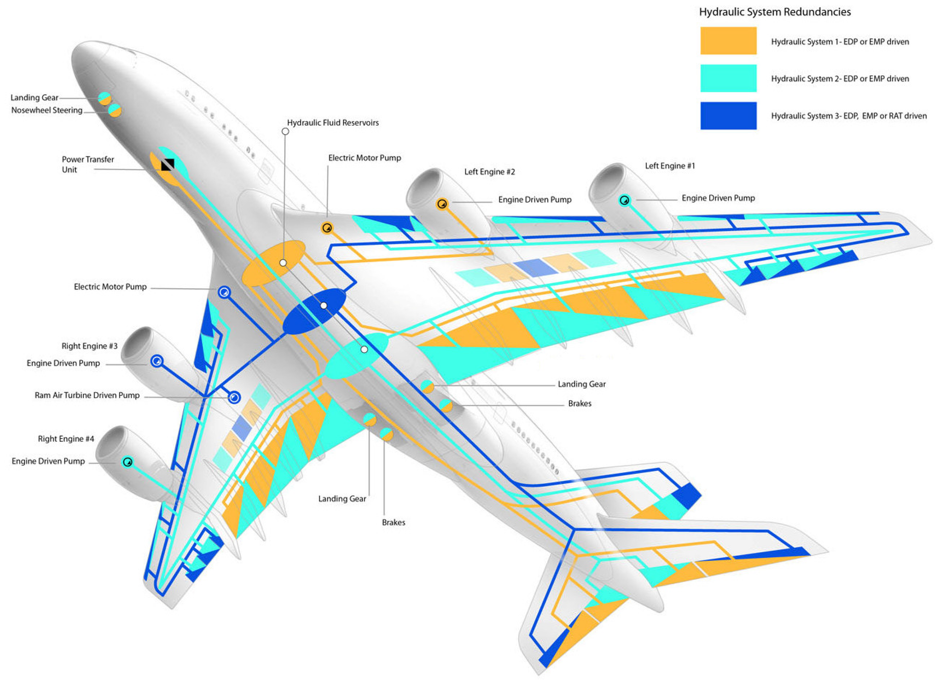
Figure 1. Structure of an aircraft hydraulic system.
Aerospace 10 00055 g001
Figure 2. An aircraft hydraulic system built by AMESIM.
Aerospace 10 00055 g002
Figure 3. Comparison between the normal state and the air pollution state.
Aerospace 10 00055 g003aAerospace 10 00055 g003b
Figure 4. EMD results of different channel signals.
Aerospace 10 00055 g004aAerospace 10 00055 g004b
Figure 5. PCA method to reduce the information.
Aerospace 10 00055 g005
Figure 6. Three different inner structures of LSTM networks.
Aerospace 10 00055 g006
Figure 7. The structure of LSTM networks for hydraulic system fault diagnose.
Aerospace 10 00055 g007
Figure 8. The flow chart of the EMD-LSTM fault diagnostic method for aircraft hydraulic system.
Aerospace 10 00055 g008
Figure 9. The confusion matrix of the three different structures of LSTM.
Aerospace 10 00055 g009aAerospace 10 00055 g009b
Figure 10. The effect of different parameters on the accuracy of fault diagnosis.
Aerospace 10 00055 g010
Figure 11. Comparison of fault state and normal state signals in different noise environments.
Aerospace 10 00055 g011
Figure 12. Comparison of EMD results of fault state signals in different noise environments.
Aerospace 10 00055 g012aAerospace 10 00055 g012b
Figure 13. Comparison of the fault diagnostic methods in different noise environments.
Aerospace 10 00055 g013
Table 1. Simulation parameters of the aircraft hydraulic system.
NumberAME-Element Key Parameter ValueMeaning
1signal03Output5000 r·min−1The shaft speed is 5000 r/min, and the pressure of the pump is 3000 psi.
3Accumulato2Gas pressure
accumulator volume
1885 psi
2.62 L
Accumulator reduces pressure, as an emergency source.
4presscontol01Relief valve cracking pressure 3436 psiPressure relief value, for system discharge.
5tank01Tank pressure 50 psiBooster tank, for pre-boost to 50 psi.
7pump13Nominal shaft speed5000 r·min−1Left engine drive pump (EDP).
11~14pump13nominal shaft speed 5000 r·min−1
4166 r·min−1
Right EDP, Yellow system EMP, Blue system EMP, and RAT. Rated pressure of RAT is 2500 psi.
10constant_3constant value34.4738 barPTU opens when the pressure difference between green and yellow systems is 34.4738 bar.
Table 2. Fault state values of the hydraulic system.
NumFault Category and Category NumberKey Parameter Normal ValueFault Value
2pump leakage-1Equivalent orifice diameter (mm)0.1~0.31~2
6filter blockage-2Equivalent orifice diameter (mm)5~73~4
7relief valve spring failure-3Open pressure (psi)34002600–3300
11Actuator inner leakage-4Leakage coefficient (L·min−1·bar−1)0~0.01 0.03~0.05
16oil pollution-5Air content (%)0.1~0.35~15
Table 3. Collection signals of six states.
PositionSignalMarkPositionSignalMark
Pump PressurePpActuatorPressurePa
FlowrateQpFlowrateQa
Oil filter PressurePfDisplacementDa
FlowrateQfVelocityVa
Table 4. Optimal parameter values for the LSTM.
Parameter NameValue
Lr0.001
Lr decayinglr = lr × 0.9/epoch
Batch size800
Dropout rate0.4
Training epochs200
Activation functionReLU
OptimizerAdam
Table 5. Different samples used for the aircraft hydraulic fault diagnosis.
Class NumberStatesFault ValueTraining
Data
Testing
Data
Sample
Length
Feature
0Normal state-800200500040
1Pump leakage1~2800200500040
2Filter blockage3~4800200500040
3Relief valve spring failure2600–3300800200500040
4Oil pollution5~15800200500040
5Actuator inner leakage0.03~0.05800200500040
Table 6. Simulation results of the three LSTM methods.
ClassAlgorithmAccuracy/%Test Time/sSoftware/Mb
1LSTM97.331.685.9
2LSTM with observation97.081.777.5
3GRU98.251.613.2
Table 7. The simulation results of different network structures.
ClassFault Diagnostic Model StructureAccuracyTest TimeMode Size
1GRU without EMD93.16%1.31 s2.6 mb
2GRU without PCA96.33%3.99 s7.3 mb
3EMD-8-GRU95.71%1.43 s10.3 mb
4EMD-GRU98.25%1.61 s3.2 mb
Table 8. The simulation results of different learning rates and batch size.
Learning rate0.10.010.0010.00010.000010.000001
Accuracy/%25.560.491.298.193.279.2
Training time/s224785116456695
Batch size10020040080012001600
Accuracy/%63.585.296.898.494.588.2
Training time/s2832091351059992
Table 9. The simulation results of different environment noises.
AlgorithmAccuracy/%
Without NoiseSNR = 70 dB SNR = 40 dB
BP73.8859.5335.91
SVM65.2655.2536.53
RF75.5266.9544.77
CNN82.9879.4150.66
LSTM92.5690.4454.47
EMD-GRU (this article)98.2595.2989.29
Disclaimer/Publisher’s Note: The statements, opinions and data contained in all publications are solely those of the individual author(s) and contributor(s) and not of MDPI and/or the editor(s). MDPI and/or the editor(s) disclaim responsibility for any injury to people or property resulting from any ideas, methods, instructions or products referred to in the content.