Study on Burning Surface Regression Algorithm under Erosive Burning Based on CT Images of Solid Rocket Motor Grain

Abstract

The presence of the erosive burning effect during the operation of a solid rocket motor (SRM) is one of the most important factors affecting the proper operation of the motor. To solve the effects of the operating process of the motor under erosive burning, a synthesis algorithm based on the actual CT images is proposed to combine the Level-set (LS) method with the minimum distance function (MDF) method for the simulation of the burning surface regression of the grain under erosive burning. The Hamilton–Jacobi control equation can be solved exactly for the discrete form of LS. To improve the computational efficiency of the LS method, the minimum distance field is initialized and only the distortion grid is adjusted during the reinitialization. The third-order TVD Runge–Kutta method is used to solve the problem of numerical oscillation and improve the calculation accuracy. The experiments simulate the burning process of the NAWC No. 6 partial grain under erosive burning, which can provide the main basis for the performance design of solid propellant. The experimental results show that the method has good applicability to three-dimensional complex grains. It can realize the simulation of grains under erosive burning and its calculation accuracy is high.

1. Introduction

The solid rocket motor (SRM) is a simple, low-cost, and highly reliable power unit that is widely used in commercial launch vehicles and various tactical and strategic missiles [1,2]. In the process of SRM design, due to its unique mode of operation, it is generally impossible to directly control its thrust magnitude, so it is necessary to design a specific shape of SRM grain to control the thrust according to a specific thrust scheme [3]. Therefore, the simulation of grain burning surface regression is one of the core problems of SRM design.

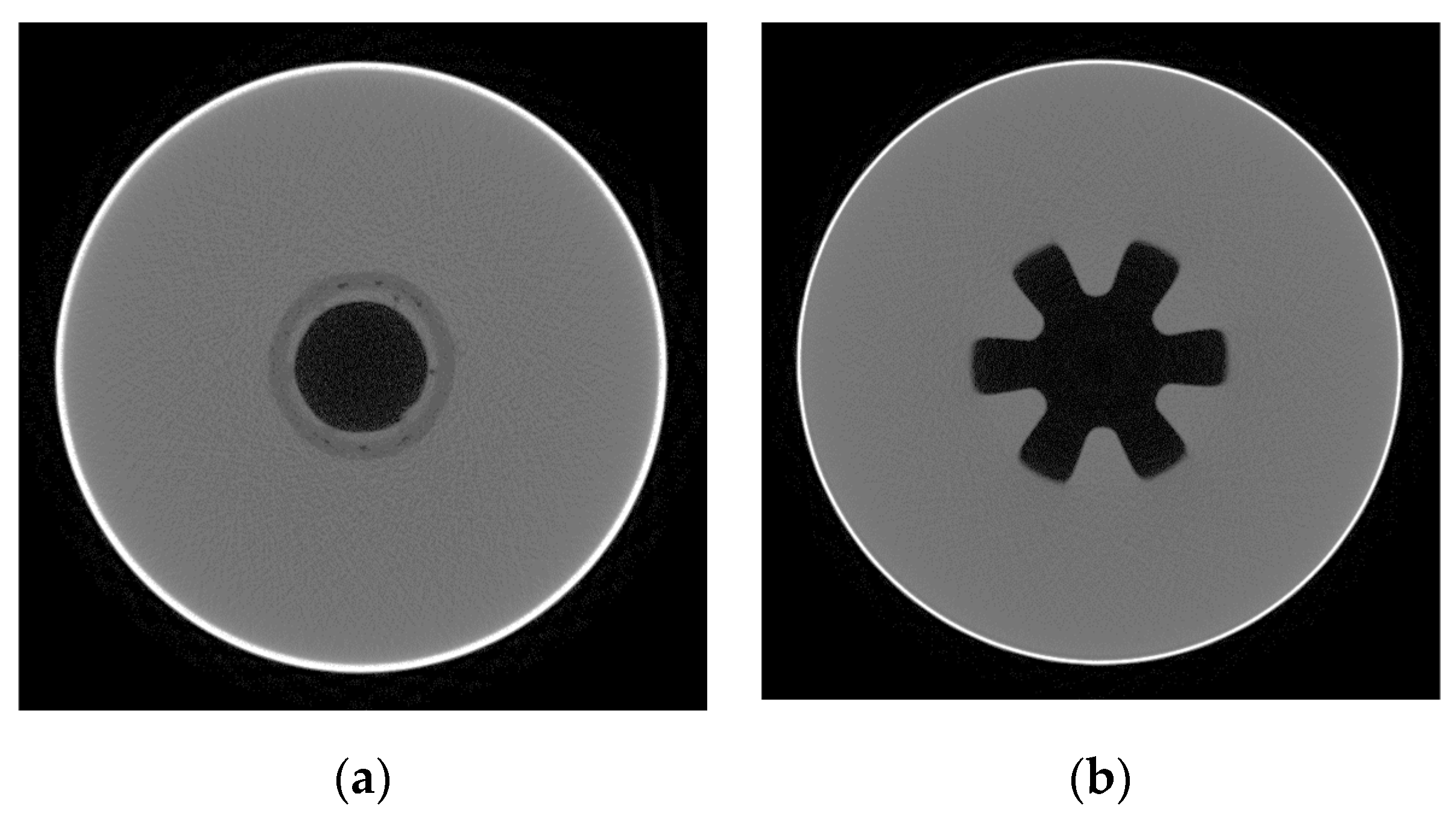
The internal surface of an SRM grain is subject to stress and strain due to manufacturing, storage, internal pressure load and other reasons, and as a result, defects are produced on the internal surface of the grain. In order to build the real internal surface of solid propellant to operate as efficiently as possible, nondestructive testing is required. Computed Tomography (CT) is an advanced technical means of inspecting SRMs, which has the characteristics of visual imaging, is high resolution, and is not limited by the geometry of the workpiece [4]. CT images can clearly show the internal structure of SRMs. The real grain data is extracted by image processing, and based on this, feature points are found. The initial burning surface is then interpolated to thicken the CT images and reconstructed as a 3D model.

For simple-shaped grains, the burning surface regression under the geometric law of burning can be calculated by the analytical geometry method, while for relatively complex-shaped grains, the burning surface regression algorithm can be used to simulate the burning process [5]. However, for an accurate prediction of SRM performance, the non-uniform distribution of burning rate in time and space must be considered, so the required burning surface regression algorithm must also support a non-uniform dynamic burning rate, which can also be interpreted as an interface tracking problem [6].

The numerical methods for solving interface tracking can be divided into two categories: explicit methods and implicit methods [7]. Explicit methods use a large number of basic elements to approximate the shape of the burning surface, and offset, merge, add and delete elements to simulate the burning surface. These include the general coordinate method [8,9], solid modeling method [10], and dynamic mesh method [11,12]. The implicit method is to define an isosurface in the field function on the grid to approximate the shape of the burning surface and to manipulate the values of the field function on the grid to offset the isosurface. Although the implicit methods consume more computational resources, they are more compatible with complex burning surfaces and rate fields, and the implicit methods such as the Level-set (LS) method [13,14,15] and the minimum distance function (MDF) method effectively avoid topology problems [16,17]. The commonly used implicit method is the LS method, which represents the real-time burning surface of the grain through the isosurface in the directed distance field, and indirectly moves the isosurface by numerical manipulation of the grid point distance field, which is theoretically applicable to any three-dimensional shape of the grain.

In recent years there have been some studies of LS methods applied to SRM burning surface regression calculations. Yildirim et al. [18] studied the effect of various factors on internal ballistics using the LS method. Dong-Hui et al. [19] took advantage of the good generality of the LS method by embedding it into a structural optimization system that can automatically generate a large number of design solutions and perform an automated evaluation. Cavallini et al. [15] calculated the entire burning process of a solid rocket motor using the quasi-one-dimensional unsteady internal ballistic coupling LS method, which is particularly suitable for calculating the internal ballistics of the motor under erosive burning. There is also a need for research scholars to study the effect of grain defects on internal ballistics using the LS method [20,21,22]. The LS method has been well applied to the simulation of grain burn-back in the above references, but the calculation speed has not been improved and the process of multiple reinitialization has not been solved. Wei et al. [23] used Boolean operations to extract the burning surface and accelerated the computation of dense regions using GPUs. Oh et al. [24] proposed a hybrid burning regression analysis method to classify and solve complex grains by selectively using the MDF method and LS method according to different needs. In these references, the speed of the LS method has been continuously improved, but the model it supports is an ideal model. The actual model may have some defects caused by manufacturing and storage, a problem which has not been resolved.

For non-uniform burning rate models, erosive burning effects are the most common important cause of the non-isometric burning surface regression. Erosive burning not only changes the direction of burning surface regression, significantly affecting the internal ballistics and performance of the motor, but also leads to premature exposure of part of the adiabatic layer [25]. Many researchers have developed erosive burning models from heat transfer mechanisms, among which, the widely used models include the Lenoir–Robillard (LR) model [26] and the Zeldovich–Novozhilov (ZN) model [27]. Willcox et al. [28] improved the LR model, which considers the thermal feedback of the gas to the grain as the pressure and flow rate of the gas. Several studies have successfully applied the LR model to investigate erosive burning effects [29,30,31]. Since the ZN model requires finite element simulation of the heat transfer process in addition to the 1D or 3D solution of the internal flow field calculation, and the high complexity of the model is not conducive to coupling with the burning surface regression algorithm, the LR model is chosen to study the erosive burning effect.

In this study, the 3D model of an SRM grain is reconstructed based on CT images, and the fusion of the LS method and MDF method is proposed to solve the problems of the LS method which requires multiple reinitializations and large computational load. The proposed method is validated in non-uniform and different burning rate grain models. Due to the presence of the erosive burning effect in SRM, the algorithm of this study is used to calculate and simulate an SRM grain with the erosive burning effect based on the LR model to verify the effect of the erosive burning on the motor propellant.

2. Models

2.1. 3D Reconstruction of CT Images

The real motor CT images are shown in Figure 1. These two images are the tube grain and star grain. In order to reconstruct the tube-to-star transition part grain of the NAWC No. 6 model, the CT image should be processed first, and the grain data and the initial burning surface of propellant should be extracted using image processing means such as filtering and threshold segmentation. Then the feature points of the initial burning surface in the image are matched using linear interpolation, and finally, the complete 3D grain is reconstructed.

Figure 2 shows the reconstructed grain using the algorithm of this paper, and Figure 2 shows the boundary part in order to provide a more intuitive view. The number of grid points used in this example is 512 × 512 × 150. The number of grid points is larger and the computational load is greater. However, as the grid is dense, its computational accuracy is also higher.

2.2. Erosive Burning Effect

Erosive burning is a burning phenomenon that is unique to solid propellants during burning. It is a phenomenon that causes an increase in the burning rate of the grain when the flow rate of the high-temperature gas flowing parallel to the burning surface reaches a certain value. Erosive burning not only generates initial pressure peaks and increases burning chamber loads but also affects motor thrust and operating time. Additionally, as the performance requirements of SRMs continue to increase, the problem of erosive burning has become more prominent. To represent the relative impact of erosive burning effects, the commonly used parameter of the erosive ratio can be defined as in Equation (1):

$$\epsilon =r/r_o=1+r_e/r_o$$

(1)

where $r_o$ is the propellant burning rate without the effect of lateral gas flow, $r$ is the actual burn rate with the effect of lateral gas flow, and $r_e$ is the difference between the basic burn rate at the same pressure, also known as the erosive burning rate.

Researchers have observed the following basic phenomena through extensive erosive burning experiments. First, the transverse gas rate and pressure passing through the burning surface of the propellant are the basic factors affecting the erosive burning rate of the propellant. The greater the cross-flow rate, the greater the erosive burning rate. At the same gas rate, the higher the pressure, the greater the burning rate. Secondly, the influence of propellant components on erosive burning is mainly shown by the influence of components on the basic burning rate. Generally, low-burning rate propellants and higher-burning-rate propellants are more sensitive to the erosive burning effect, which is the same for double-base propellants and composite propellants.

The central gas flow heat transfer model proposed by Lenoir and Robillard is representative of the surface heat transfer theory. It is believed that erosive burning is caused by the convective heat transfer on the propellant surface that results from the high-temperature gas flow in the center of the motor channel. The LR model has two basic assumptions: one is that the erosive burning is proportional to the heat transfer rate of the central gas flowing to the propellant surface; and the other is that the total burning rate is the superposition of basic burning rate and erosive burning rate without the effect of the cross flow. The LR model can be expressed by Equations (2) and (3):

$$r=r_0+r_e=a{p}^n+\alpha \frac{G^{0.8}}{D^{0.2}}{e}^{-\frac{\beta r_0{\rho }_c}{G}}$$

(2)

$$\alpha =\left[0.0288C_{pg}{\mu }_g^{0.2}{\mathrm{Pr}}^{-2/3}\right]\frac{1}{{\rho }_c{C}_{pc}}\left(\frac{T_f-T_s}{T_s-T_o}\right)$$

(3)

where $a{p}^n$ is the basic burning rate under non-erosive burning; $a$ is a scale constant; $G=\rho u$ is the dense flow of gas; $D$ is the characteristic size of the section, generally taken as the distance from the grain head; $\beta$ is a constant whose empirical value is about 53; $C_{pg}$ is the specific heat at constant pressure; $C_{pc}$ is the specific heat of the solid propellant; $\mathrm{Pr}$ is the Prandtl number; $T_f$ is the adiabatic flame temperature; $T_s$ is the burning surface temperature; $T_o$ is the initial temperature; ${\rho }_c$ is the density of the propellant; and ${\mu }_g$ is the viscosity of burning products. The value of $\alpha$ in Equation (3) can also be derived from empirical data and needs to be corrected due to fluctuations in the values that occur near sudden changes in the ventilation area.

For large SRMs, the LR model overestimates the contribution of the erosive burning effect. The reason for this over-prediction is that the characteristic length in Equation (2) uses the distance from the head, which can be further improved as the empirical formula in Equation (4):

$$f\left(D_h\right)=0.9+0.189D_h\left[1+0.043D_h\left(1+0.023D_h\right)\right]$$

(4)

3. Methods

3.1. Level-Set Method

In reality, there are a lot of moving interface problems, also known as Stefan problems [32]. Simulating and tracking the moving interface is the key to solving this problem. The method to solve the moving state of the moving interface can be called the interface tracking algorithm. The burning surface calculation of solid propellant can also be regarded as a kind of interface tracking problem. The LS method adds an additional dimension to the initial interface to describe the interface motion. It uses the implicit functions $\phi \left(t\right)$ to represent the active interface. The isosurface in the directed distance field is used to represent the burning surface of the grain. The numerical value in the directed distance field is operated to move the isosurface indirectly, the implicit function of the higher dimension is adjusted according to the surface motion $\phi \left(t\right)$, and then the isosurface is calculated to obtain the position of the moving interface (Figure 3).

The solid area is set as ${\mathsf{\Omega }}_s$, the gas area as $\overline{\mathsf{\Omega }}$, and the interface as $\mathsf{\Gamma }$. The function φ is defined to calculate the conforming distance from any point in the region to the interface, as shown in Equation (5).

$$\left\{\begin{array}{c}\begin{array}{ccc}\phi \left(x,y,t\right)>0& in& {\mathsf{\Omega }}_s\end{array}\\ \begin{array}{ccc}\phi \left(x,y,t\right)=0& on& \mathsf{\Gamma }\end{array}\\ \begin{array}{ccc}\phi \left(x,y,t\right)<0& in& \overline{\mathsf{\Omega }}\end{array}\end{array}\right.$$

(5)

Each node in the calculation area changes with the movement of the interface, so the derivative of the coordinates on the interface with respect to $t$ can be expressed as Equation (6).

$${\phi }_t+F\sqrt{{\phi }_x^2+{\phi }_y^2}=0$$

(6)

It is assumed that the curve evolves along the normal direction, according to the interface rate field $\overrightarrow{V}$. To ensure that the isosurface of the function φ is the active interface at any moment, it is necessary to satisfy the conservation Equation (7).

$$\frac{\partial \phi }{\partial t}+F\cdot \nabla \phi =0$$

(7)

The LS method can easily handle the case of boundary intersections. As in Figure 4, the two circular interfaces gradually recede into a larger circular interface and intersect and merge.

3.2. Numerical Solution

In order to solve for the partial derivatives of the function φ, a common first-order method is the Godunov format, where the partial derivatives corresponding to the three axes are combined to calculate the $\left|\nabla \phi \right|$ of the LS method. Since the computational process of the LS method is discretized, it is theoretically impossible to find a completely accurate analytical solution through discrete grid points, and this computational process is estimated from the grid point data for $\nabla \phi$. In order to maintain the convergence and stability of the solution, the Hamilton–Jacobi equation is chosen for the control equation of the LS method [33]. The form of the viscosity calculation for this equation satisfying the entropy condition is given in Equation (8):

$${\phi }_{ijk}^{n+1}={\phi }_{ijk}^n-\mathsf{\Delta }t\left[\max \left(F_{ijk},0\right){\nabla }^{+}+\min \left(F_{ijk},0\right){\nabla }^{-}\right]$$

(8)

where $\nabla$ is the central difference equation, as shown in Equations (9) and (10):

$$\begin{array}{cc}{\nabla }^{+}=& (\max {\left(D_{ijk}^{-x},0\right)}^2+\min {\left(D_{ijk}^{+x},0\right)}^2+\\ & \max {\left(D_{ijk}^{-y},0\right)}^2+\min {\left(D_{ijk}^{+y},0\right)}^2+\\ & \max {\left(D_{ijk}^{-z},0\right)}^2+\min {\left(D_{ijk}^{+z},0\right)}^2{)}^{1/2}\end{array}$$

(9)

$$\begin{array}{cc}{\nabla }^{-}=& (\max {\left(D_{ijk}^{+x},0\right)}^2+\min {\left(D_{ijk}^{-x},0\right)}^2+\\ & \max {\left(D_{ijk}^{+y},0\right)}^2+\min {\left(D_{ijk}^{-y},0\right)}^2+\\ & \max {\left(D_{ijk}^{+z},0\right)}^2+\min {\left(D_{ijk}^{-z},0\right)}^2{)}^{1/2}\end{array}$$

(10)

where h is the spatial step size. $D_{ijk}^{-x}=\frac{{\phi }_i-{\phi }_{i-1}}{h},D_{ijk}^{+x}=\frac{{\phi }_{i+1}-{\phi }_i}{h}$ and so on.

To improve the accuracy of the time direction, time discretization is also performed using the TVD Runge–Kutta time discretization format [34,35]. A one-step Eulerian forward advance is calculated by Equation (11), followed by another advance in the same way.

$$\frac{{\phi }^{n+2}-{\phi }^{n+1}}{\mathsf{\Delta }t}+F_n\cdot \left|\nabla \phi \right|=0$$

(11)

The results of the two steps are then averaged as in Equation (12).

$${\phi }^{n+\frac{1}{2}}=\frac{3}{4}{\phi }^n+\frac{1}{4}{\phi }^{n+2}$$

(12)

After obtaining the value at moment $n+1/2$, the Eulerian forward advance can be performed to obtain the value at moment $n+3/2$ (see Equation (13)).

$$\frac{{\phi }^{n+\frac{3}{2}}-{\phi }^{n+\frac{1}{2}}}{\mathsf{\Delta }t}+F_n\cdot \left|\nabla \phi \right|=0$$

(13)

Finally, the final desired value of $n+1$ moments can be obtained by a single averaging operation (see Equation (14)).

$${\phi }^{n+1}=\frac{1}{3}{\phi }^n+\frac{2}{3}{\phi }^{n+\frac{3}{2}}$$

(14)

3.3. MDF Initialization

Before solving the LS method, the motor model needs to mesh so that the grain and the flow field region are decomposed into small cell bodies, and the composition isosurface $\mathsf{\Gamma }\left(t\right)$ is obtained and discretized according to the divided mesh. The minimum distance operation is performed on the whole mesh to obtain the new ${\phi }_0$.

The initial MDF value of each 3D grid node is calculated, and the distance sign of each grid point is discriminated according to whether it is inside the grain or not. Since the initial burning surface and the end surface of the grain column on each slice are closed and non-self-intersecting irregular shapes, the rules for determining the grid point symbols can be assigned by discerning whether they are inside the initial burning surface and the termination surface. The ray method is used to determine that the point is inside the polygon. The main idea of this algorithm is to make a ray in any direction with the target point as the endpoint, usually in the x+ direction. The number of intersection points of this ray with the polygon are counted. If it is technical, the target point is inside the polygon, and if it is even, the target is outside the polygon.

The distance value of each grid point is difficult and computationally intensive, and an efficient data structure is needed to quickly search for the minimum distance from the grid point to be calculated to the burning surface. The nearest neighbor algorithm in machine learning provides a K-d tree, which is a spatial division data structure often used for searching in high-dimensional spaces. The basic idea of the K-d tree is similar to that of the binary tree but differs in that each node represents a sample. The sample is divided into different nodes by selecting a certain dimensional feature in the sample, first sorted by the x coordinate. The middle x_mid is selected as the root node, and then the points smaller than x_mid are in the left subtree, and those larger than x_mid are in the right subtree. Then the left and right subtrees are sorted by the y coordinate, and so on (see Figure 5).

The minimum distance method obtained by directly judging the minimum distance from the grid to the discrete points of the interface does not need to consider complex geometric operations. However, the minimum distance obtained has a certain error with the actual distance, and the error is larger when it is near the burning surface and smaller when it is far from the interface. In order to reduce the calculation error and improve the calculation efficiency at the same time, the distance is discriminated in the form of point-to-surface when the grid point is close to the burning surface (i.e., the distance between the grid point and the burning surface is less than 10 times the space step), and the minimum distance value is obtained directly by the KNN algorithm when the grid point is far from the burning surface. The maximum error of the minimum distance value of the point far from the burning surface should not exceed 1.25%.

When the grid points are close to the burning surface, the three nearest discrete points are selected to form the surface, as shown in Figure 6, and can be divided into three cases. The first case: When the point p is located in region I, this case is the distance from the point to the face. The second case: When the point p is located in region II, this case is the distance from the point to the line segment. The third case: When point p is located in region III, this can be approximated as the distance from point p to the nearest point.

3.4. Reinitialization

The numerical results of the solution should be such that the function $\phi \left(x\right)$ remains as a function of the distance to the interface with compliance. In a rate field with rate $\overrightarrow{r}$, it is difficult to avoid the deviation of the function $\phi \left(x\right)$ from the sign of the distance to the interface during the calculation, especially in the case where the gradient of $\phi \left(x\right)$ becomes large or small near the isosurface. In order to reduce such errors, a general method needs to be introduced to make the function $\phi \left(x\right)$ keep the distance with the symbol to the isosurface at all times, thus avoiding bias. The commonly used method is to iteratively converge the function $\phi \left(x\right)$ by substituting it into a specific partial differential equation [36].

The interface $\mathsf{\Gamma }\left(t\right)=\left\{x:\phi (x,t)=0\right\}$ no longer depends on the specific initial value $\phi \left(x,0\right)$ selected, only that the initial value selected matches $\mathsf{\Gamma }\left(0\right)$. The reinitialization process is to replace the old function with a new one and both have the same isosurface. However, the characteristics of the new function will be better than the old one to avoid value shifts, and when the new function is obtained it will be used as the initial value to continue the computation until the next reinitialization process is performed [37]. A better way of solving the Hamilton–Jacobi equation to obtain the new function is described here, and its computational equation is shown in Equation (15) [37].

$$\left\{\begin{array}{c}d+S(d_0)\left(\left|\nabla d\right|-1\right)=0\\ d\left(x,0\right)=d_0\left(x\right)=\phi \left(x,t\right)\end{array}\right.$$

(15)

The solution of this equation is the optimal symbolic distance after reinitialization, and the computation of grid points near the interface converges very quickly in the actual computation, or the definition shown in Equation (16) can be used.

$$S\left(\phi \right)=\frac{d}{\sqrt{d^2+{\delta }^2}}$$

(16)

From the accuracy point of view, the synthesis algorithm process does not introduce errors from the gradient estimation process, so the accuracy of this method is no less than that of the general method. In terms of calculation speed, the efficiency of the composite algorithm relative to the horizontal set method depends on whether it takes less time to initialize (rebuild the directed distance field using the geometric method) than it does to reinitialize (until the calculation converges). Obviously, when each step backward makes the directed distance field more distorted, the synthesis algorithm is more efficient. Due to this feature, the synthesis algorithm is more suitable for those pills with more sharp geometric shapes and more discontinuities in the velocity field. The test results show that the synthesis algorithm and the level set method have basically the same compatibility and accuracy. The difference is only that the two methods have different efficiencies for input data with different characteristics.

Figure 7 shows the iterative process of the two algorithms. The LS method is based on narrowband technology, and when a certain step is calculated, points near the $\phi (x)=0$ interface need to be reinitialized to either 0 or 1 or −1, then iteration continues. The main errors during this period come from reinitialization errors and the inaccuracy of $\phi (x)=0$ updates when there is a gradient that is too large or too small in the iteration. The main error of the synthesis algorithm comes from the error of the first calculation of the distance between the grid points. The difference of the distance between the grid points near $\phi (x)=0$ conforms to the curvature of the surface. Therefore, when iterating, the difference distance is passed to other grid points as a ripple. The value on the grid points always maintains its distance from the $\phi (x)=0$ interface, and the symbol can be used to determine whether it is on the solid or gaseous side.

4. Results and Discussion

4.1. Computational Environment

Our synthesis algorithm performs separate performance tests in non-uniform and uniform burning cases, including tube grains, star grains, tube-to-star articulated partial grains in NAWC No. 6 grains, and different burn rate tube grains to verify non-uniform burning. The grain is modeled by 3D CT images and the VTK open-source library, and the initial burning surface can be easily extracted by an edge detection algorithm. The mesh model is then planned and the entire 3D model is iterated using the synthesis algorithm. The code for the synthesis algorithm was written in Visual Studio 2022 platform using c++, and all test results were run on a Window 10 OS computer configured with Intel i7-10700 (2.90 GHz) and 16G RAM.

4.2. NAWC No. 6 Partial Grain

The complex irregular part of the NAWC No. 6 grain is selected for the feasibility verification of the algorithm. Figure 8 shows the results of the calculations for the tube-to-star grain in the synthesis algorithm. From this process, it can be seen that the star burning surface is larger and gradually affects the tube burning surface during the burning process. Some propellant will be left in the star cross-section at the later stage of burning, resulting in some propellant remaining in the tube cross-section as well.

Figure 9 shows the change in the area of the burning surface of the NAWC No. 6 partial grain during the burning process. In comparison with the LS method, it can be seen that the synthesis algorithm in this study has less computational error. Since the synthesis algorithm does not require frequent initialization of the mesh, the calculation is more stable when the burning surface changes less regularly. Both the synthesis algorithm and the LS method can be used to calculate the burning surface regression for the actual motor grain to provide a basis for the internal ballistics of the motor grain, and are equally applicable to irregular grains.

4.3. Tube Grain

A computational simulation of tube grain under erosive burning effect was performed using the synthesis algorithm. It can be visualized from Figure 10 that at the beginning of the burning phase, the overall motor burning rate is high and the erosive burning effect is obvious. In the late stage of the burning, the gas channel shows a small front and large rear cone, and the erosive burning effect almost disappears. Although the erosive burning effect disappears in the later stages of the work, the conical channel formed at the beginning continues to have an effect, which causes an early reduction of the burning surface in the final stages of the work.

Figure 11 shows the calculation with the erosive burning effect compared with the calculation with the geometrical law of burning. Since erosive burning mainly occurs at the early stage of motor operation, the erosive burning effect can have a profound effect on the later operating condition of the motor. The erosive burning severely affects the peak burning area of the tube grain, with the result that the motor fails to reach the theoretical level of operation, and the burning surface gradually decreases in the later stages of operation, which may lead to abnormal motor thrust.

4.4. Star Grain

Figure 12 shows the burning process of the star grain under the erosive burning effect. The length of this model is small, but it can still be seen that the rear half of the grain produces a conical surface under the erosive burning effect. The effect of erosive burning on the star grain can be visualized in Figure 13. The erosive burning causes the peak burning area to be advanced and the peak pressure to be advanced. The remaining grain appears when the star grain is about to burn out, and the erosive burning significantly shortens the burning time of the star grain column, which then seriously affects the motor′s working condition.

4.5. Different Burning Rate Grain

In practice, there are multiple pouring batches in large motors, resulting in deviations in the burn rate of each part of the grain causing deviations in the burn surface curve. This example is for the problem of calculating the burning surface of a grain with different burning rates. The grain is a tube grain and is wrapped at both ends. This example assumes that the grain has two different burning rates. In order to show the burning rate gradient more clearly and to make the basic calculation of the grain column easily using the geometric analysis method, this example assumes that the high burning rate is double the low burning rate.

From Figure 14, it can be seen that after burning, the high burning rate grain area seriously affects the low burning rate area, and the burning surface forms an obvious step-like shape. In the second half of the burning period, the high burn rate area is burned out and the burning surface is sharply reduced. There is still some burning surface in the low-burning rate part of the grain.

It can be seen from Figure 15 that the theoretical values of the synthesis algorithm and the geometric-analytical method are very close with small errors. Near the peak of the burning surface area, the synthesis algorithm is slightly less than the theoretical value because the burning surface is extracted and the surface is smoother. The synthesis algorithm provides a certain judgment basis for the different burning rate of grains caused by different batches of pouring, and can provide a basis for the waste judgment standard and fault diagnosis of multi-burning-rate grains.

From the simulations of the above experimental cases, it can be seen that the synthesis algorithm has the advantages of the LS method for three-dimensional topology and incorporates the MDF method to reduce the high operational load of reinitialization. It can deal with the burning surface regression calculation of three-dimensional complex grains and non-uniform burning grains, and has good applicability.

4.6. 0-D Simulations

The change of gas pressure in the chamber is determined by the gas generation rate, the gas mass flow rate discharged from the nozzle and the gas mass change rate in the chamber. This is a complex process in which grain burning and gas flow interact. To simplify this process, the average values of flow parameters along the axis are taken regardless of their distribution along the axis, which is the meaning of 0-D internal ballistic calculation. The pressure use Equation (17) for the combustor is solved in the fourth-order Runge–Kutta time scheme:

$$\frac{V_g}{{\mathsf{\Gamma }}^2{C}_{\ast }^2}\frac{dp}{dt}={\rho }_p{A}_{b}a{p}^n\phi \left(\zeta \right)-\frac{\phi p{A}_t}{C_{\ast }}$$

(17)

where $V_g$ is the free volume of the chamber, ${\rho }_p$ is the propellant grain density, $A_b$ is the grain burning area, $r_o=a{p}^n$ is the average burning speed of the grain, $\phi \left(\zeta \right)$ is the erosive burning correction factor, $\phi$ is the flow correction factor, $C_{\ast }$ is the characteristic velocity, and $A_t$ is the nozzle throat area. $\mathsf{\Gamma }$ is calculated with isentropic choked nozzle conditions by Equation (18):

$$\mathsf{\Gamma }={\left(\frac{2}{k+1}\right)}^{\frac{k+1}{2(k-1)}}\sqrt{k}$$

(18)

where $k$ is the specific heat capacity ratio of gas.

Generally, the pressure trace of the SRM follows the trend of the total burning surface area of the grain after the ignition transient stability. Figure 16 and Figure 17 show the 0-D internal ballistic pressure curves of the NAWC No. 6 partial grain and star grain. It can be seen that this part of the grain is basically in conformity with this rule. After a short initial pressure peak (approximately 13 ms), the pressure change increases with the increase in the total burning area. The erosive burning effect increases the average burning rate of the grain during the early working period, resulting in an increase in the peak initial pressure. It also causes the peak pressure to come earlier in the late working phase and shortens the total operating time of the motor.

5. Conclusions

The purpose of this study was to develop a practical 3D grain burning surface regression algorithm based on CT images to reduce the computation time and improve the accuracy of the calculation. A synthesis method was proposed to solve for tracking the moving burning surface using a combination of the LS method and the MDF method. The LS method helps the accuracy of interface tracking, but it is computationally intensive and requires frequent reinitialization of the problem. The MDF method is fast in computation and the problem of frequent reinitialization can be solved by correcting the minimum distance field, which reduces the computational load. The synthesis algorithm effectively exploited the advantages of both methods.

The algorithm developed in this study was validated through the computational simulation of the burning surface regression of the conventional SRM. For the analysis and calculation of irregular and complex three-dimensional grains and grains with different burning rates under the erosive burning effect, the results show that the synthesis algorithm proposed in this study has high applicability and high calculation accuracy. This algorithm could be coupled with internal ballistic calculations in subsequent studies for internal ballistic analysis of solid propulsion systems.

In subsequent research, we will use CT images of SRMs with defects to reconstruct the three-dimensional grain model with defects, including common failure modes such as cavitation, debonding, and cracks. Image processing methods will be used to locate the defects and improve the synthesis algorithm, making it suitable for the simulation of burning surface regression of the grain with defects. The influence of defects on the performance of the grain will be analyzed to simulate the state of the motor when it is working.

References

1. Dhital, D.; Lee, J.R.; Farrar, C.; Mascarenas, D. A review of flaws and damage in space launch vehicles: Motors and engines. J. Intell. Mater. Syst. Struct. 2014, 25, 524–540. [Google Scholar] [CrossRef]
2. Le, A.Q.; Sun, L.Z.; Miller, T.C. Health monitoring and diagnosis of solid rocket motors with bore cracks. J. Aerosp. Eng. 2016, 29, 3. [Google Scholar] [CrossRef]
3. Shun, L.; Hongyi, L.; Weiwei, Z.; Bin, Z.; Yucheng, Y.; Doudou, S. Fast algorithm for grain burnback of actual shaped grains of solid motor. J. B Univ. Aeronaut. Astronaut. 1–13.
4. Fu, Q.; Zhao, J. An Automatic Method to detect defects for Solid Rocket Motor. In 2015 International Conference on Applied Science and Engineering Innovation; Atlantis Press: Jinan, China, 2015; pp. 1935–1939. [Google Scholar]
5. Wanzhi, H. Simulation of the Transient Internal Flow of SRM with the Grain Surface Regression Based on Level-Set Method. Master’s Thesis, Harbin Engineering University, Harbin, China, 2016. [Google Scholar]
6. Fei, Q. Method Research for Burning Surface Calculation of Solid Rocket Motor with Complicated Grain. Master’s Thesis, Northwestern Polytechnical University, Xi’an, China, 2003. [Google Scholar]
7. Ran, W. Research on Algorithms for Dynamic Nonuniform Regression of Solid Rocket Motors and Its Application. Ph.D. Thesis, Northwestern Polytechnical University, Xi’an, China, 2019. [Google Scholar]
8. Barron, J. Generalized coordinate grain design and internal ballistics evaluation program. In Proceedings of the 3rd Solid Propulsion Conference, Atlantic City, NJ, USA, 4–6 June 1968; p. 490. [Google Scholar]
9. Coats, D.E.; Levine, J.N.; Nickerson, G.R.; Tyson, T.J.; Cohen, N.S.; Price, C.F. A Computer Program for the Prediction of Solid Propellant Rocket Motor Performance; Ultrasystems Environmental Inc.: Irvine, CA, USA, 1975; Volume 3. [Google Scholar]
10. Wei, L. Calculation of the Interior Ballistic Performance of Solid Rocket Motor Based on Pro/E and Qt. Master’s Thesis, Harbin Engineering University, Harbin, China, 2014. [Google Scholar]
11. Voller, V.R.; Brent, A.D.; Prakash, C. The modelling of heat, mass and solute transport in solidification systems. Int. J. Heat Mass Transf. 1989, 32, 1719–1731. [Google Scholar] [CrossRef]
12. Jiao, X. Face offsetting: A unified approach for explicit moving interfaces. J. Comput. Phys. 2007, 220, 612–625. [Google Scholar] [CrossRef] [Green Version]
13. Sethian, J.A. Theory, algorithms, and applications of level set methods for propagating interfaces. Acta Numer. 1996, 5, 309–395. [Google Scholar] [CrossRef] [Green Version]
14. Hegab, A.; Jackson, T.L.; Buckmaster, J.; Stewart, D.S. Nonsteady burning of periodic sandwich propellants with complete coupling between the solid and gas phases. Combust. Flame 2001, 125, 1055–1070. [Google Scholar] [CrossRef]
15. Cavallini, E.; Favini, B.; Di Giacinto, M.; Serraglia, F. Internal ballistics simulation of a NAWC tactical SRM. J. Appl. Mech. 2011, 78, 051018. [Google Scholar] [CrossRef] [Green Version]
16. Willcox, M.A.; Brewster, M.Q.; Tang, K.C.; Stewart, D.S. Solid propellant grain design and burnback simulation using a minimum distance function. J. Propul. Power 2007, 23, 465–475. [Google Scholar] [CrossRef]
17. Ren, P.; Wang, H.; Zhou, G.; Li, J.; Cai, Q.; Yu, J.; Yuan, Y. Solid rocket motor propellant grain burnback simulation based on fast minimum distance function calculation and improved marching tetrahedron method. Chin. J. Aeronaut. 2021, 34, 208–224. [Google Scholar] [CrossRef]
18. Yildirim, C.; Aksel, H. Numerical simulation of the grain burnback in solid propellant rocket motor. In Proceedings of the 41st AIAA/ASME/SAE/ASEE Joint Propulsion Conference & Exhibit, Tucson, AZ, USA, 10–13 July 2005; p. 4160. [Google Scholar]
19. Dong-Hui, W.; Yang, F.; Fan, H.; Wei-Hua, Z. An integrated framework for solid rocket motor grain design optimization. Proc. Inst. Mech. Eng. Part G 2014, 228, 1156–1170. [Google Scholar] [CrossRef]
20. Fei, Q.; Guangqiang, H.; Peijin, L.; Jiang, L. A New Algorithm for Burning Surface Calculation of Solid Rocket Motor with Complicated Grain Based on Level set Method. J. Northwest. Polytech. Univ. 2005, 4, 456–460. [Google Scholar]
21. Yang, F. Analysis on the Performance of Solid Rocket Motor with Cracked Propellant Grain. Master’s Thesis, National University of Defense Technology, Changsha, China, 2010. [Google Scholar]
22. Tshokotsha, M.H. Internal Ballistic Modelling of Solid Rocket Motors Using Level Set Methods for Simulating Grain Burnback. Ph.D. Thesis, Stellenbosch University, Stellenbosch, South Africa, 2016. [Google Scholar]
23. Wei, R.; Bao, F.; Liu, Y.; Hui, W. Combined acceleration methods for solid rocket motor grain burnback simulation based on the level set method. Int. J. Aerosp. Eng. 2018, 2018, 4827810. [Google Scholar]
24. Oh, S.H.; Lee, H.J.; Roh, T.S. Development of a hybrid method in a 3-D numerical burn-back analysis for solid propellant grains. Aerosp. Sci. Technol. 2020, 106, 106103. [Google Scholar] [CrossRef]
25. Wei, R.; Bao, F.; Liu, Y.; Hui, W. Precise Design of Solid Rocket Motor Heat Insulation Layer Thickness under Nonuniform Dynamic Burning Rate. Aerosp. Sci. Technol. 2019, 2019, 5789430. [Google Scholar] [CrossRef]
26. Godon, J.C.; Duterque, J.; Lengelle, G. Solid-propellant erosive burning. J. Propul. Power 1992, 8, 741–747. [Google Scholar] [CrossRef]
27. DeLuca, L.; Di Silvestro, R.; Cozzi, F. Intrinsic combustion instability of solid energetic materials. J. Propul. Power 1995, 11, 804–815. [Google Scholar] [CrossRef]
28. Willcox, M.A.; Brewster, M.Q.; Tang, K.C.; Stewart, D.S.; Kuznetsov, I. Solid rocket motor internal ballistics simulation using three-dimensional grain burnback. J. Propul. Power 2007, 23, 575–584. [Google Scholar] [CrossRef] [Green Version]
29. Landsbaum, E.M. Erosive burning of solid rocket propellants-a revisit. J. Propul. Power 2005, 21, 470–477. [Google Scholar] [CrossRef]
30. Rettenmaier, A.; Heister, S. Experimental Evaluation of Erosive Burning in a Planar Combustor. In Proceedings of the 47th AIAA/ASME/SAE/ASEE Joint Propulsion Conference & Exhibit, San Diego, CA, USA, 31 July–3 August 2011; p. 5564. [Google Scholar]
31. Weaver, J.; Gauthier, J.D.; Stowe, R. Transient Chamber Flowfield Simulation of a Rod-and-Tube Configuration Solid Rocket Motor. In Proceedings of the 40th AIAA/ASME/SAE/ASEE Joint Propulsion Conference and Exhibit, Fort Lauderdale, FL, USA, 11–14 July 2004; p. 4179. [Google Scholar]
32. Ruxun, L.; Zhifeng, W. Numerical Simulation Methods and Motion Interface Tracking, 1st ed.; University of Science and Technology of China Press: Hefei, China, 2001; pp. 194–206. [Google Scholar]
33. Osher, S.; Sethian, J.A. Fronts propagating with curvature-dependent speed: Algorithms based on Hamilton-Jacobi formulations. J. Comput. Phys. 1988, 79, 12–49. [Google Scholar] [CrossRef] [Green Version]
34. Shu, C.W.; Osher, S. Efficient implementation of essentially non-oscillatory shock-capturing schemes. J. Comput. Phys. 1988, 77, 439–471. [Google Scholar] [CrossRef] [Green Version]
35. Osher, S.; Fedkiw, R.; Piechor, K. Level set methods and dynamic implicit surfaces. Appl. Mech. Rev. 2004, 57, B15. [Google Scholar] [CrossRef] [Green Version]
36. Chen, Y.G.; Giga, Y.; Goto, S. Uniqueness and existence of viscosity solutions of generalized mean curvature flow equations. Proc. Jpn. Acad. Ser. A 1989, 65, 207–210. [Google Scholar] [CrossRef]
37. Sussman, M.; Fatemi, E.; Smereka, P.; Osher, S. An improved level set method for incompressible two-phase flows. Comput. Fluids 1998, 27, 663–680. [Google Scholar] [CrossRef]
Figure 1. Partial CT images of NAWC No. 6 grain: (a) tube grain; (b) star grain.
Aerospace 10 00021 g001
Figure 2. Grain reconstructed based on CT image.
Aerospace 10 00021 g002
Figure 3. Schematic diagram of the LS implicit function φ.
Aerospace 10 00021 g003
Figure 4. Cross integration of two interfaces.
Aerospace 10 00021 g004
Figure 5. K-d tree sorting diagram.
Aerospace 10 00021 g005
Figure 6. Judgment of distance from near point to burning surface. Regions I–III represent three cases of projection of grid nodes to the nearest burning surface triangle element.
Aerospace 10 00021 g006
Figure 7. Iteration process diagrams: (a) LS method; and (b) synthesis algorithm.
Aerospace 10 00021 g007
Figure 8. Burning process of NAWC No. 6 partial grain.
Aerospace 10 00021 g008
Figure 9. Comparison the burning surface area of the synthesis algorithm and LS algorithm in NAWC No. 6 partial grain.
Aerospace 10 00021 g009
Figure 10. Burning process of tube grain under erosive burning.
Aerospace 10 00021 g010
Figure 11. Comparison of the burning area of tube grains under erosive burning and under geometrical law of burning.
Aerospace 10 00021 g011
Figure 12. The burning process of star grain under erosive burning.
Aerospace 10 00021 g012
Figure 13. Comparison of burning area of star grains under erosive burning and under geometrical law of burning.
Aerospace 10 00021 g013
Figure 14. Burning process of double burning-rate tube grain.
Aerospace 10 00021 g014
Figure 15. Comparison of the burning surface area of geometric theoretical value with synthesis algorithm under erosive burning and under geometrical law of burning.
Aerospace 10 00021 g015
Figure 16. 0-D internal ballistic P-T diagram of NAWC No. 6 partial grain under the synthesis algorithm.
Aerospace 10 00021 g016
Figure 17. 0-D internal ballistic P-T diagram of Star grain under synthesis algorithm.
Aerospace 10 00021 g017
Disclaimer/Publisher’s Note: The statements, opinions and data contained in all publications are solely those of the individual author(s) and contributor(s) and not of MDPI and/or the editor(s). MDPI and/or the editor(s) disclaim responsibility for any injury to people or property resulting from any ideas, methods, instructions or products referred to in the content.