Assessment of Climatic Parameters for Future Climate Change in a Major Agricultural State in India

Abstract

The change in future climate will have a prominent impact on crop production and water requirement. Crop production is directly related to climatic variables. Temperature, solar radiation, wind, precipitation, CO₂ concentration and other climatic variables dictate crop yield. This study, based on long-term historical data, investigates the patterns and changes in climatic variables (precipitation, temperature, and solar radiation) that would most significantly affect the future crop production in many parts of the world, and especially in India, where most farmers depend on rainfall for rice production. Statistical analyses—box and whisker plot, mean absolute error, Taylor diagram, double mass curve, Mann–Kendall trend test, and projected climate change—were used to assess the significance of the climatic factors for the purpose of agricultural modeling. Large variability in precipitation may cause the flash floods and affect the farming, and at the same time, increase in temperature from baseline period will lead to high water requirement by crops, and may cause drought if rainfall does not occur. Decrease in solar radiation will affect crop growth and development, and thus, would hamper the crop production. The results of this study would be useful in identifying the negative issues arising from climate change in future agricultural practices in Bihar, India. Furthermore, the results can also help in developing management strategies to combat the climate change impact on crop production.

1. Introduction

The occurrence of climate change is being recognized all across the world [1]. The change in climate will potentially impact the global population by altering agricultural production [2,3]. Since the weather is a decisive factor for agricultural production, change in climate will affect the crop growth, yield, and water requirement. The future climate projection for South Asia by the Intergovernmental Panel on Climate Change presents that the average annual temperature will increase by 3–6 °C and 2–3 °C with worst case scenario (RCP 8.5) and low emission scenario (RCP 2.6), respectively, by the end of the 21st century [4], and the change in precipitation will depend upon the location of any study [5].

The process of assessing the impact of climate change on agriculture depends on the climate data (precipitation, maximum and minimum temperature, and solar radiation), apart from environmental, social and economic aspects [6]. The future conditions, called future scenarios, are the central decision-making situations used by the policy and decision makers to explore the change in the climate first, and then use those trends to develop strategies for climatic resiliency. These scenarios are defined based on population growth, economic development, social aspects and advancement in new technologies [7,8,9]. Therefore, climate scenarios will continue to change during each generation and need to be modified by policymakers and scientists at a certain interval. The Intergovernmental Panel on Climate Change (IPCC) 5th report [10] included advanced sets of climate scenarios that have considered all the aspects mentioned above, which have been expressed as the Representative Concentration Pathways (RCPs) and replaced all the scenarios from previous reports.

With an ever-increasing global population, the demand for increasing food production has increased substantially [11]. However, the patterns of change in climatic variables pose challenges in not only increasing crop production level, but even maintaining the current yield levels [12,13,14]. The problem intensifies for regions where majority of the people depend on agriculture, and climate change has already disrupted current agricultural production practices [15,16]. The degree of climate change in India varies from one region to another and will, thereby, affect agricultural production [17]. Our study focused on the State of Bihar in India, where the livelihoods of more than 80% of people rely on agriculture. The future climate will govern crop production, and thereby, livelihood of its people [12]. Recent frequent droughts, flooding, crop damage, and uncertainties in precipitation amount and timing have posed significant challenges in sustainability of the farming system in Bihar [18]. Bihar and its agricultural practices are unique. Farmers are mostly marginal and have no control of changing their rice production practices [19]. The state is facing severe water and climate crises, and hence, this study was aimed at investigating the climate change parameters specific for this study area, and recommending if the production practices need to be shifted/changed in order for a sustainable farming community. Our study will provide the rationale for employing the outcomes of this study to analyze the impact on agricultural production for the state of Bihar and to develop strategies for future production practices.

Therefore, in this study, we focused on how change in climate data can be assessed for agricultural management policies. We used the baseline observed climate data of Agricultural Model Intercomparison and Improvement Project (AgMIP) Modern-Era Retrospective Analysis for Research and Applications (AgMERRA), suitable for agricultural studies, with current climate change scenarios provided by IPCC 5th assessment report, and the simulated climate data through General Circulation Models (GCMs) of Coupled Model Intercomparison Project (CMIP5). Thus, the objectives of this study were set to (i) analyze the variations in climate data simulated by various General Circulation Models (GCMs), (ii) establish a relationship between observed and model-simulated data, and to observe the future climate trend from all the four used GCMs and (iii) project a total climate change from the ensemble mean of all the GCMs, in order to use with any crop production model, and to make the crop production and water management strategies.

2. Material and Methods

2.1. Study Area Description and Agricultural Dataset for Crop Modeling

The study area, state of Bihar, is shown in Figure 1 with its elevation. The river Ganges divides the state into two parts, flowing from west to east. The climate of Bihar is Humid Sub-Tropical with an average annual rainfall of 1297 mm, mainly received in the monsoon season (June to September).

2.2. Climatic Datasets and Correction Methodology

The climate data for this study were obtained from the website of Climate Change, Agriculture and Food Security (CCAFS) (www.ccafs-climate.org/data/ (accessed on 31 May 2021)), developed by Consultative Group on International Agricultural Research (CGIAR), under a research program addressing the climate change impact on agricultural production. The AgMERRA, a high-resolution (0.25° × 0.25°) daily time-series climate dataset, has been used in CCAFS data portal to simulate future climate data through CMIP5 GCMs, for the purpose of agriculture modeling [20,21,22,23]. Therefore, the AgMIP Modern-Era Retrospective Analysis for Research and Applications (AgMERRA) baseline (historical) data from 1980–2004 (25 years) were used as an available observed data on this website to generate the simulated baseline, and future climate data of 40 years (2020–2059). Four GCMs (bcc_csm1_1, csiro_mk3_6_0, ipsl_cm5a_mr, miroc_miroc5) available in the Coupled Model Intercomparison Project (CMIP5) were used in this study to obtain the simulated baseline and future climate data on a daily basis.

Based on recent recommendations of future climate change scenarios, Representative Concentration Pathways (RCPs)—RCP 2.6, RCP 4.5, RCP 6.0, and RCP 8.5 by IPCC 5th assessment report—we selected all four of them for our investigation in this study.

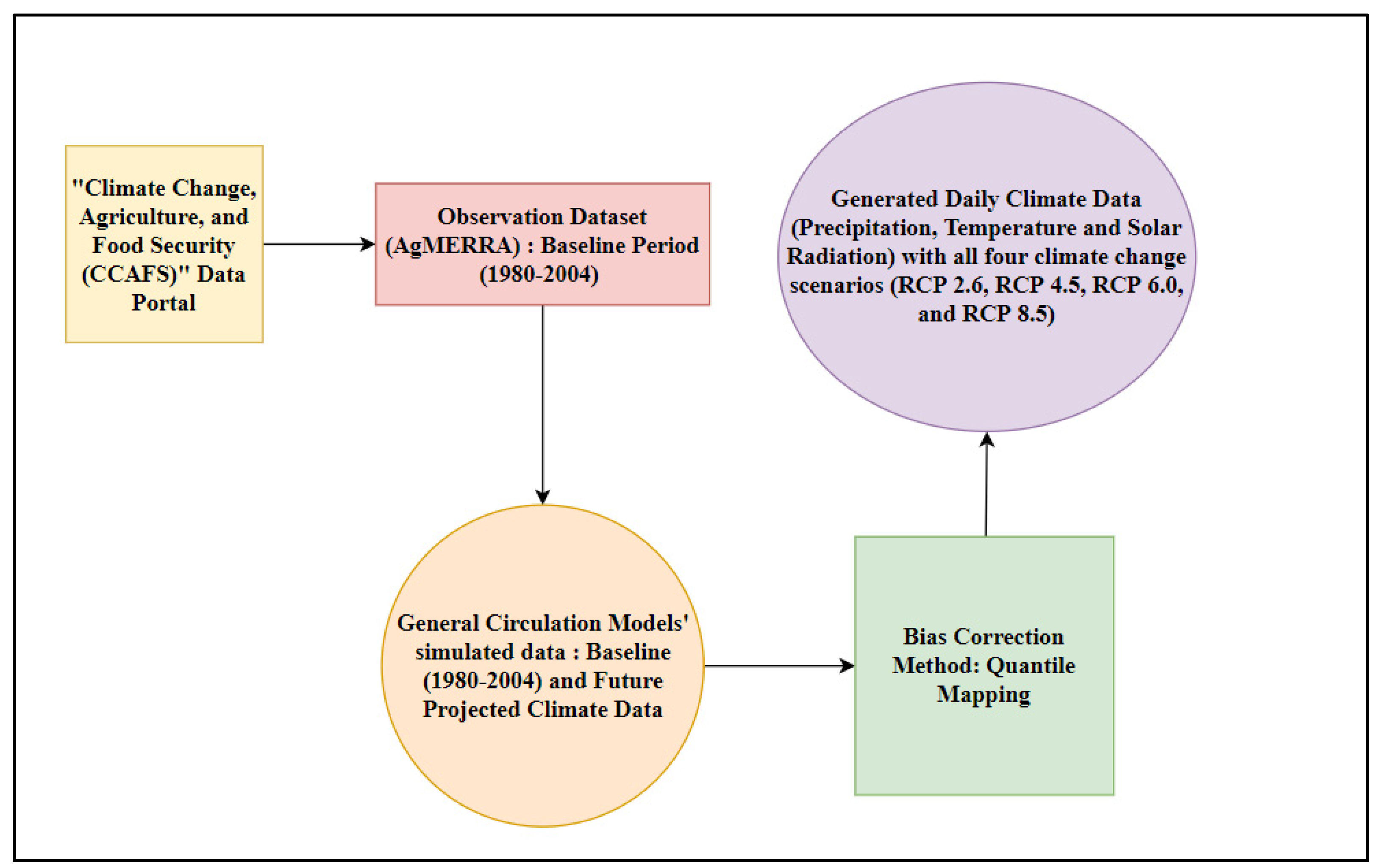
Before using the GCMs’ produced climate data for crop modeling, errors and biases need to be corrected in order to avoid the ambiguity in climate change impact results [24]. The methods of correcting these errors and biases from the climate data are called “bias correction methods,” those are based on adjusting the long-term mean and variability of GCM simulated outputs using observed data as the benchmark for the correction [20]. There are several bias correction methods; however, in this study, we used the quantile mapping method to correct the GCMs’ output data, to remove the biases and systematic errors through minimizing the differences between observed and predicted variables, based on the established relationships between cumulative density functions. The flow chart of obtaining climate data is illustrated in Figure 2. This has been described in detail by Jha et al. [12].

2.3. Ensemble Mean Method

In order to study the overall approximate change in climate, the ensemble mean of climate data of four selected GCMs was estimated. This method led us to compute the average of all four climate models’ projection with all the four climate change scenarios. This ensemble mean of climate data was used for assessing the variation in climate with box and whisker plot, and to estimate the projected climate change with all the four climate change scenarios.

2.4. Statistical Analysis of Climate Data

2.4.1. Box and Whisker Diagram (Variation in Historical Simulated Data)

To investigate the distribution of historical simulated data from 1980–2004, box and whisker plots for all the climatic factors were developed. The plots were developed on a monthly basis from the ensemble mean of all the four models. The visualization of the box and whisker plot provided information about the central tendency (median), variability range, skewness and extremity of the data [25]. The extreme values at both ends of the scale, called outliers, indicated the extension from a larger range of the data. The purpose of using the box and whisker plot was to show the variability in the data, free from the assumptions of the normal distribution.

2.4.2. Mean Absolute Error (Evaluation of Models’ Performance)

Mean absolute error, a useful statistical measure, was used to evaluate model’s performance. We used both, MAE and RMSE, to study the models’ performance for simulation of climate data. RMSE was shown in the plot of the Taylor diagram, while the MAE was computed independently. Distribution of weight to all errors are equal in MAE, while RMSE gives more weight to errors with large absolute values compared to errors with smaller absolute values [26]. It was calculated from Equation (1).

$$MAE=\frac{1}{n}{\displaystyle \sum }_{I=1}^n\left|X_i-\overline{X_i}\right|$$

(1)

where n = number of errors, $\left|X_i-\overline{X_i}\right|$ = absolute error.

2.4.3. Taylor Diagram (Association between Observed and Simulated Climate Data)

The Taylor diagram established a statistical relationship between observed and GCMs’ simulated data to show their performance for simulating the climatic variables [27]. The graphical illustration of the association between observed and simulated data was assessed in terms of their correlation, centered root-mean-square error and the standard deviation. An abbreviated name was assigned to each model, after computing the statistics for all the four GCMs. The position of each abbreviated name on the plot quantifies how closely the models’ simulated data for each variable match with the observation data. In a quadrant, the values represented on the dashed arc show the correlation. The climate models lie on or between the straight line coming from corresponding arc values demonstrate the correlation between observed and simulated data. The radial distance from the origin presents the standard deviation between observed and simulated data, and distance from the observed point on the x-axis illustrates the centered root-mean-square error (CRMSE).

The statistics that provide the degree of correspondence between simulated and observed data in the Taylor diagram were calculated using the formula below:

The correlation coefficient, R (Equation (2)), between observed and simulated climate data was estimated from Equation (2).

$$\mathrm{R}=\frac{\raisebox{1ex}{$1$}\!\left/ \!\raisebox{-1ex}{$\mathrm{N}$}\right.\left({\mathrm{S}}_{\mathrm{n}}- \overline{\mathrm{S}}\right)\left({\mathrm{O}}_{\mathrm{n}}- \overline{\mathrm{O}}\right)}{{\mathsf{\sigma }}_{\mathrm{s}}-{\mathsf{\sigma }}_{\mathrm{o}}}$$

(2)

The centered root mean square error (CRMSE) between observed and simulated climate data was computed using Equation (3).

$$\mathrm{CRMSE}=\sqrt{\frac{1}{\mathrm{N}}{\displaystyle \sum }_{\mathrm{n}=1}^{\mathrm{N}}{\left[\left({\mathrm{S}}_{\mathrm{n}}- \overline{\mathrm{S}}\right)-\left({\mathrm{O}}_{\mathrm{n}}- \overline{\mathrm{O}}\right)\right]}^2}$$

(3)

The standard deviations of the simulated (σ_s) and observed (σ_o) climate data were estimated from Equations (4) and (5).

$${\mathsf{\sigma }}_{\mathrm{s}}=\sqrt{\frac{1}{\mathrm{N}}{\displaystyle \sum }_{\mathrm{n}=1}^{\mathrm{N}}{\left({\mathrm{S}}_{\mathrm{n}}- \overline{\mathrm{S}}\right)}^2}$$

(4)

$${\mathsf{\sigma }}_{\mathrm{o}}=\sqrt{\frac{1}{\mathrm{N}}{\displaystyle \sum }_{\mathrm{n}=1}^{\mathrm{N}}{\left({\mathrm{O}}_{\mathrm{n}}-\overline{\mathrm{O}}\right)}^2}$$

(5)

where S_n and O_n are simulated and observed values at nth days; N is the total number of days; $\overline{\mathrm{S}}$ and $\overline{\mathrm{O}}$ are the average values of the total period.

2.4.4. Mann–Kendall Trend Test (Establishing a Trend in Future Climate Data)

The Mann–Kendall trend test [28,29], a non-parametric rank-based procedure, as a most appropriate test, was used to determine the positive or negative trends in the climatic variables [30]. This method is also suitable for finding the trend with non-normally distributed time series data, which contain outliers and nonlinear trends [31]. A confidence limit of 95% was used as a monotonic trend test for this study. The null hypothesis (H_o) for the assessment assumed that there was no trend in the climatic variables for the future period (2020–2059). Thus, the null hypothesis was rejected if p < 0.05. The alternate hypothesis (H₁) assumed a significant positive or negative trend in climate data. The steps followed to compute trend in the climate are as follows:

The Mann–Kendall statistic, S, of the data series, x, was calculated using Equation (6).

$$\mathrm{S}={\displaystyle \sum }_{\mathrm{i}=1}^{\mathrm{n}-1}{\displaystyle \sum }_{\mathrm{j}=\mathrm{i}+1}^{\mathrm{n}}\mathrm{sgn} \left({\mathrm{x}}_{\mathrm{j}}-{\mathrm{x}}_{\mathrm{i}}\right)$$

(6)

where sgn is the signum function, and n is the total number of data. The standard deviation associated with S was calculated from Equation (7).

$$\mathrm{SD} \left[\mathrm{S}\right]=\sqrt{\frac{1}{18} [\mathrm{n}\left(\mathrm{n}-1\right)\left(2\mathrm{n}+5\right)-{\displaystyle \sum }_{\mathrm{j}=1}^{\mathrm{k}}{\mathrm{t}}_{\mathrm{j}}\left({\mathrm{t}}_{\mathrm{j}}-1\right)\left(2{\mathrm{t}}_{\mathrm{j}}+5\right)}$$

(7)

where k represents the number of tied groups in the data set, and t_j is the number of data points in group j. However, in this case, n (40 years) was greater than 10, and thus, SD [S] was calculated using the given Equation (8).

$$\mathrm{SD} \left[\mathrm{S}\right]=\sqrt{\frac{1}{18} [\mathrm{n}\left(\mathrm{n}-1\right)\left(2\mathrm{n}+5\right)}$$

(8)

The presence of statistically significant trend was evaluated using the Z value obtained from Equation (9).

$$\mathrm{Z}=\{0\begin{array}{c}\frac{\mathrm{S}-1}{\mathrm{SD}\left[\mathrm{S}\right]} \mathrm{if} \mathrm{S}>0 \\ \mathrm{if} \mathrm{S}=0\\ \frac{\mathrm{S}+1}{\mathrm{SD}\left[\mathrm{S}\right]} \mathrm{if} \mathrm{S}<0 \end{array}$$

(9)

A positive value of Z indicated an increasing trend in the data series, while a negative Z represents a decreasing trend. Then, the Theil-Sen’s slope approach [32], a non-parametric procedure, was applied to quantify the trend in data series. The slope Q between any two values of a data series x was estimated using Equation (10).

$$\mathrm{Q}=\frac{{\mathrm{x}}_{\mathrm{j}}-{\mathrm{x}}_{\mathrm{k}}}{\mathrm{j}-\mathrm{k}}, \mathrm{j}\ne \mathrm{k}$$

(10)

where x_j and x_k represent the data values at time j and k (j > k), respectively. The Sen’s slope for the complete dataset would be the median of all the N values of Q; where$\mathrm{N}=\frac{\mathrm{n}\left(\mathrm{n}-1\right)}{2}$, n is the number of years. Therefore, the overall Sen’s slope is computed from Q_f (Equation (11)).

$${\mathrm{Q}}_{\mathrm{f}}=\mathrm{f}\left(\mathrm{x}\right)=\{\begin{array}{c}{\mathrm{Q}}_{\left(\raisebox{1ex}{$\mathrm{N}+1$}\!\left/ \!\raisebox{-1ex}{$2$}\right.\right)} \mathrm{if} \mathrm{N} \mathrm{is} \mathrm{odd}\\ \frac{{\mathrm{Q}}_{\raisebox{1ex}{$\mathrm{N}$}\!\left/ \!\raisebox{-1ex}{$2$}\right.}+{\mathrm{Q}}_{\left(\raisebox{1ex}{$\mathrm{N}+2$}\!\left/ \!\raisebox{-1ex}{$2$}\right.\right)}}{2} \mathrm{if} \mathrm{N} \mathrm{is} \mathrm{even}\end{array}$$

(11)

At the end, the final slope is estimated by a two-tailed test at 100% (1-α) confidence interval.

2.4.5. Double Mass Curve (Consistency Between Observed and Simulated Climate Data)

The double mass curve was used to check the consistency between observed and predicted results of precipitation and solar radiation data for all the four global climate models. This method consisted of the plot between two cumulative quantities for the same period. The slope of the straight line in this plot represents the proportionality between the two quantities. Plotting of 1:1 line provides the insight of biases between the observed and predicted data and captures the period where inconsistency can be observed. The correction of the data was performed by adjustment of the slope, if it was needed. The division of the average of cumulative quantity on Y-axis by X-axis provided the slope to correct the inconsistency in data.

The relationship between both the quantities on X and Y axes is represented by Y = bX, where b is the slope of the double mass curve. If an inconsistency was observed from a change in the slope of the straight line, correction was made by dividing the predicted precipitation or multiplying the observed precipitation by the slope. Slope to adjust the straight line is computed by the division of cumulative average of predicted and observed rainfall.

2.4.6. Projected Climate Change

The projected future climate change was computed to describe the expected change in the climatic variables during a specific time-period with climate change scenarios from the baseline period (1980–2004). In this study, the projected change in future climate for 10 years of the interval from 2020–2059 was calculated for the climate change scenarios, RCP 2.6, RCP 4.5, RCP 6.0, and RCP 8.5, for each of the GCMs. Further, the ensemble mean of all the four climate models were used to illustrate overall projected change. The projected climate change for each of the scenarios was estimated on a monthly basis for the 10 years of the interval using Equation (12). The average of monthly estimation for 10 years of the future segment was subtracted from the average of the baseline period (1980 –2004), provided the expected future change in a particular climatic variable.

$$\begin{gathered} \mathrm{Future} \mathrm{change} \mathrm{for} \mathrm{every} 10 \mathrm{years} \mathrm{of} \mathrm{interval} \\ =(\mathrm{Average} \mathrm{of} \mathrm{climate} \mathrm{projection} \mathrm{for} 10 \mathrm{years} \mathrm{of} \mathrm{interval} \\ - \\ \mathrm{Average} \mathrm{of} \mathrm{baseline} \mathrm{period}) \end{gathered}$$

(12)

3. Results

3.1. Variability in Historical Data

Figure 3 illustrates the monthly climate variability for the baseline period (1980–2004) of 25 years, obtained from the ensemble mean of all the four GCMs, in which the monthly variation in precipitation datasets for the baseline period is shown in Figure 3a. In winter season (November–March), maximum precipitation varies between 19.54 mm/month and 44.08 mm/month. The median of precipitation in winter season lies between 7.83 mm/month and 14.03 mm/month, and the interquartile range (IQR) changes between 4.77 mm/month and 9.78 mm/month. The maximum precipitation in monsoon season (June–September) reaches around 500 mm/month, and the median of precipitation changes between 50 mm/month and 266 mm/month.

Figure 3b demonstrates the median, dispersion, skewness, and extremes in maximum temperature for each month during the historical period. IQR for the winter season varies from 0.45 °C/month to 0.85 °C/month, and the median of the maximum temperature lies between 24.27 °C/month and 27.37 °C/month. Further, IQR in the monsoon season observes a variation from 0.54 °C/month to 1.90 °C/month, with the median of maximum temperature changing from 32.46 °C/month to 36.25 °C/month. The extremes of maxima and minima were observed to be 38 °C/month and 34 °C/month, respectively, in the monsoon season. In addition to that, Figure 3c presents the variability in minimum temperature obtained from the ensemble mean of all the four models for the historical period. Winter season observes the change in the median of minimum temperature between 9.95 °C/month and 12.03 °C/month, and the change in IQR for this period was observed from 0.52 °C/month to 0.79 °C/month. Median of minimum temperature in pre-monsoon season increases from 16.80 °C/month to 21.57 °C/month, and IQR changes from 0.80 °C/month to 0.95 °C/month. The highest and lowest in minimum temperature were observed to be 27 °C/month and 24.50 °C/month, respectively, in the monsoon season. The difference in the median of minimum temperature between each month in monsoon season is very minimum, while IQR lies between 0.31 °C/month and 0.44 °C/month.

Furthermore, the variability in solar radiation can be seen from Figure 3d. Maximum and minimum solar radiation in monsoon season was observed to be 21.26 MJ/m²/month and 14 MJ/m²/month, respectively, and IQR varies between 0.76 MJ/m²/month and 1.47 MJ/m²/month. Median of solar radiation in winter season changes between 16 MJ/m²/month and 21 MJ/m²/month, with the change in IQR from 1–1.94 MJ/m²/month. The minimal extreme of solar radiation was observed to be 13 MJ/m²/month² in the winter season.

3.2. Evaluation of Models’ Performance

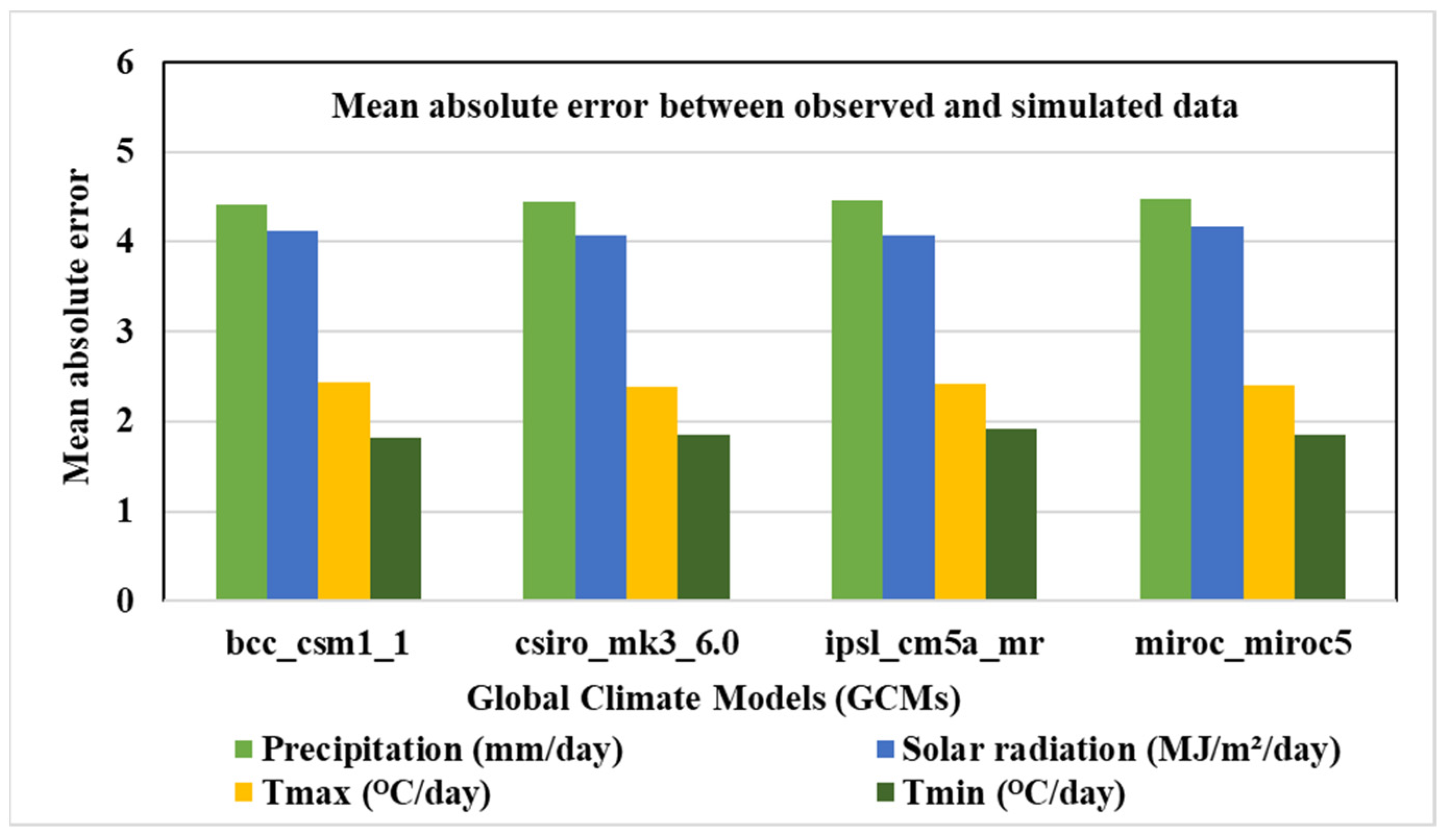
Figure 4 shows the mean absolute error between observed and simulated historical data for climatic factors (precipitation, temperature, and solar radiation) with all the GCMs. The maximum and minimum error were computed to be 4.47 mm/day and 4.42 mm/day with miroc_miroc5 and bcc_csm1_1, respectively. The maximum error with daily solar radiation data was found to be 4.17 MJ/m²/day with miroc_miroc5, and minimum error was estimated to be 4.07 MJ/m²/day with csiro_mk3_6_0. For maximum temperature, the largest error of 2.43 °C/day was calculated with bcc_csm1_1, while the smallest error of 2.39 °C/day was estimated with csiro_mk3_6_0. The highest mean absolute error for a minimum temperature of 1.92 °C/day was observed with ipsl_cm5a_mr, and the smallest error of 1.82 °C/day was shown by bcc_csm1_1.

3.3. Association between Observed and Simulated Climate Data

Figure 5a displays the statistical relationships between observed and simulated precipitation for the baseline period (1980–2004) with all the four selected climate models (bcc_csm1_1, csiro_mk3_6_0, ipsl_cm5a_mr, and miroc_miroc5). The correlation between simulated and observed precipitation for all the four models lie between 0.38 to 0.43. The model, csiro_mk3_6_0, shows a maximum correlation between observed and simulated precipitation of 0.43, and miroc_miroc5 exhibits the lowest correlation of 0.38. The highest root-mean-square error of 10 mm/day was observed with ipsl_cm5a_mr, while the smallest error of 9.62 mm/day was observed with csiro_mk3_6_0. The standard deviation of precipitation simulated by bcc_csm1_1 was found to be 8.76 mm/day, similar to the standard deviation of the observed dataset.

The correlation between observed and simulated maximum temperature was obtained in the range of 0.75 to 0.79 for all the four GCMs (Figure 5b). Among all the four models, csiro_mk3_6_0 shows the maximum correlation of 0.79. Further, the root-mean-square error value of 3.76 °C/day was found to be largest for bcc_csm1_1, and the lowest value of 3.52 °C/day was observed with csiro_mk3_6_0. The standard deviation for the miroc_miroc5 was computed to be 5.32 °C/day, relatively higher compared to the variation of 5.04 °C/day with observed maximum temperature.

Moreover, Figure 5c illustrates that ipsl_cm5a_mr has the highest correlation of 0.96 and has lowest RMS error among all the four models, whereas bcc_csm1_1 has the lowest correlation of 0.91 with observed minimum temperature and has the largest RMS error of 2.89 °C/day.

Nevertheless, with solar radiation (Figure 5d), miroc_miroc5 shows the relatively large correlation value of 0.51 MJ/m²/day, while bcc_csm1_1 has a relatively low correlation value of 0.45. The RMS error for miroc_miroc 5 was found to be 5.52 MJ/m²/day, lowest amongst all the four GCMs, while bcc_csm1_1 showed the highest RMS error of 5.86 MJ/m²/day. The amplitude of the variations (i.e., the standard deviation) for ipsl_cm5a_mr is comparatively better than all the other three models.

3.4. Establishing Climatic Variables Trend for All the GCMs

Table 1. Mann–Kendall trend test for precipitation (2020–2059) with all the four climate change scenarios.

GCMs	bcc_csm1_1			csiro_mk3_6_0			ipsl_cm5a_mr			miroc_miroc5
Climate Change Scenarios	Sen’s Slope	p-Value	Significance	Sen’s Slope	p-Value	Significance	Sen’s Slope	p-Value	Significance	Sen’s Slope	p-Value	Significance
RCP 2.6	3.721	0.048	Yes	–1.038	0.412	No	–1.872	0.042	Yes	–0.983	0.316	No
RCP 4.5	7.623	0.326	No	–0.925	0.215	No	–1.743	0.043	Yes	–1.559	0.041	Yes
RCP 6.0	6.227	0.031	Yes	–1.067	0.046	Yes	0.841	0.215	No	–3.192	0.323	No
RCP 8.5	9.810	0.005	Yes	1.723	0.265	No	3.483	0.118	No	–0.824	0.275	No

Note: Sen’s slope (mm/year).

,

Table 2. Mann–Kendall trend test for maximum annual temperature (2020–2059) with all the four climate change scenarios.

GCMs	bcc_csm1_1			csiro_mk3_6_0			ipsl_cm5a_mr			miroc_miroc5
Climate Change Scenarios	Sen’s Slope	p-Value	Significance	Sen’s Slope	p-Value	Significance	Sen’s Slope	p-Value	Significance	Sen’s Slope	p-Value	Significance
RCP 2.6	0.009	0.206	No	0.013	0.211	No	–0.035	0.101	No	–0.014	0.022	Yes
RCP 4.5	0.008	0.214	No	0.041	0.025	Yes	–0.019	0.251	No	0.005	0.372	No
RCP 6.0	0.013	0.029	Yes	0.046	0.024	Yes	–0.006	0.196	No	0.004	0.214	No
RCP 8.5	0.027	0.001	Yes	0.052	0.142	No	–0.013	0.048	Yes	–0.014	0.022	Yes

Note: Sen’s slope (°C/year).

,

Table 3. Mann–Kendall trend test for minimum annual temperature (2020–2059) with all the four climate change scenarios.

GCMs	bcc_csm1_1			csiro_mk3_6_0			ipsl_cm5a_mr			miroc_miroc5
Climate Change Scenarios	Sen’s Slope	p-Value	Significance	Sen’s Slope	p-Value	Significance	Sen’s Slope	p-Value	Significance	Sen’s Slope	p-Value	Significance
RCP 2.6	0.007	0.214	No	0.025	0.009	Yes	0.019	0.001	Yes	0.015	0.270	No
RCP 4.5	0.024	0.002	Yes	0.048	0.001	Yes	0.026	0.000	Yes	0.034	0.001	Yes
RCP 6.0	0.021	0.014	Yes	0.035	0.012	Yes	0.023	0.003	Yes	0.025	0.000	Yes
RCP 8.5	0.032	0.000	Yes	0.059	0.001	Yes	0.077	0.001	Yes	0.041	0.002	Yes

Note: Sen’s slope (°C /year).

and

Table 4. Mann–Kendall trend test for solar radiation (2020–2059) with all the four climate change scenarios.

GCMs	bcc_csm1_1			csiro_mk3_6_0			ipsl_cm5a_mr			miroc_miroc5
Climate Change Scenarios	Sen’s Slope	p-Value	Significance	Sen’s Slope	p-Value	Significance	Sen’s Slope	p-Value	Significance	Sen’s Slope	p-Value	Significance
RCP 2.6	–0.009	0.032	Yes	0.016	0.211	No	–0.035	0.101	No	–0.014	0.022	Yes
RCP 4.5	–0.011	0.020	Yes	0.014	0.025	Yes	–0.019	0.251	No	0.005	0.372	No
RCP 6.0	–0.019	0.003	Yes	0.000	0.024	Yes	–0.006	0.196	No	0.004	0.214	No
RCP 8.5	–0.025	0.002	Yes	0.000	0.142	No	–0.013	0.048	Yes	–0.014	0.022	Yes

Note: Sen’s slope (MJ/m²/year).

present the results of the Mann–Kendall trend test for all climatic variables. Table 1 shows the precipitation trend from all the four models from 2020 to 2059. With the low greenhouse gases emission scenario, RCP 2.6, both the models, bcc_csm1_1 and ipsl_cm5a_mr, showed a significant trend in precipitation change during 2020–2059, since p-value was found to be less than 0.05. The climate model, bcc_csm1_1, showed a positive trend of 3.721 mm/year, while ipsl_cm5a_mr demonstrated the negative trend of 1.872 mm/year during 2020–2059. No significant trends were observed with the other two models, csiro_mk3_6_0 and miroc_miroc5, because p-values with both of these models were found to be 0.412 and 0.316, respectively. The total annual precipitation for intermediate climate change scenario, RCP 4.5, shows decreasing trends of 1.743 mm/year and 1.559 mm/year with the models, ipsl_cm5a_mr, and miroc_miroc5, respectively. In contrast, bcc_csm1 and csiro_mk3_6_0 did not exhibit a significant trend for precipitation change with RCP 4.5. With RCP 6.0, the climate models, bcc_csm1_1 and csiro_mk3_6_0, showed the positive and negative trend of 6.227 mm/year and 1.067 mm/year, respectively. The other models did not demonstrate a significant trend in precipitation change from 2020 to 2059. Furthermore, the trend test for RCP 8.5 showed an increase in precipitation of 9.810 mm/year with the model, bcc_csm1_1, reflecting the dominance in precipitation change amongst all the models. All the other three GCMs with this scenario did not present any significant trend in precipitation change.

Table 2 demonstrates an increasing trend of 0.026 °C/year for maximum temperature with miroc_miroc5 under RCP 2.6. The other climate models did not produce significant trend for change in maximum temperature for RCP 2.6. With intermediate scenario, RCP 4.5, an increasing trend of 0.041 °C/year, 0.020 °C/year, and 0.017 °C/year were observed with csiro_mk3_6_0, ipsl_cm5a_mr, and miroc_miroc5, respectively. The model, bcc_csm1_1, were not showing a significant trend for the change in maximum temperature. All the four models, bcc_csm1_1, csiro_mk3_6_0, ipsl_cm5a_mr, and miroc_miroc5, illustrated the significant trend of 0.013 °C/year, 0.046 °C/year, 0.022 °C/year and 0.019 °C/year, respectively, with climate change scenario, RCP 6.0. The worst case scenario shows the increase of 0.027 °C/year, 0.043 °C/year, and 0.031 °C/year in maximum temperature with bcc_csm1, ipsl_cm5a_mr, and miroc_miroc5, respectively.

The trend in minimum temperature during 2020–2059 is shown in Table 3. For RCP 2.6, csiro_mk3_6_0, ipsl_cm5a_mr, and miroc_miroc5 showed a positive trend of 0.025, 0.019, 0.015, respectively. The p-value with bcc_csm1_1 was found to be higher than 0.05. Thus, it did not exhibit a significant trend in minimum temperature during 2020–2059. The trend for annual minimum temperature demonstrates the increasing trend with all the models for other scenarios, RCP 4.5, RCP 6.0, and RCP 8.5. The increase in minimum temperature is expected to increase by 0.024 °C/year, 0.048 °C/year, 0.026 °C/year, and 0.034 °C/year with bcc_csm1_1, csiro_mk3_6_0, ipsl_cm5a_mr, and miroc_miroc5, respectively, for RCP 4.5. Increasing trends of 0.021 °C/year, 0.035 °C/year, 0.023 °C/year, and 0.025 °C/year were observed with the models, bcc_csm1_1, csiro_mk3_6_0, ipsl_cm5a_mr, and miroc_miroc5, respectively, for RCP 6.0, showed a somewhat similar trend as RCP 4.5. The rate of increase in annual minimum temperature for worst case scenario, RCP 8.5, is higher compared to intermediate scenarios, RCP 4.5 and RCP 6.0. The increase in minimum temperature for RCP 8.5 was computed to be 0.032 °C/year, 0.059 °C/year, 0.077 °C/year, and 0.041 °C/year with the GCMs, bcc_csm1_1, csiro_mk3_6_0, ipsl_cm5a_mr, and miroc_miroc5, respectively.

Table 4 illustrates the trend test of solar radiation for all the four models. The models, bcc_csm1_1 and miroc_miroc5, showed a negative trend of 0.009 MJ/m²/year and 0.014 MJ/m²/year, respectively, with low emission scenario, RCP 2.6. The p-values with the other two models, csiro_mk3_6_0 and ipsl_cm5a_mr, were found to be 0.211 and 0.101, respectively, and reveal no significant trend in solar radiation. With RCP 4.5, intermediate scenario, bcc_csm1_1 was showing the decreasing trend of 0.011 MJ/m²/year, while csiro_mk3_6_0 showed the increasing trend of 0.014 MJ/m²/year. The other two models, ipsl_cm5a_mr and miroc_miroc5, did not express a significant trend in solar radiation from 2020 to 2059. The decreasing trends of 0.019 MJ/m²/year and 0.006 MJ/m²/year were observed with bcc_csm1_1 and csiro_mk3_6_0, respectively, for RCP 6.0. Trend in solar radiation for RCP 8.5 decreases by 0.025MJ/m²/year, 0.013 MJ/m²/year, and 0.014 MJ/m²/year from 2020–2059, with the models, bcc_csm1_1, ipsl_cm5a_mr, and miroc_miroc5, respectively.

3.5. Consistency between Observed and Simulated Climate Data

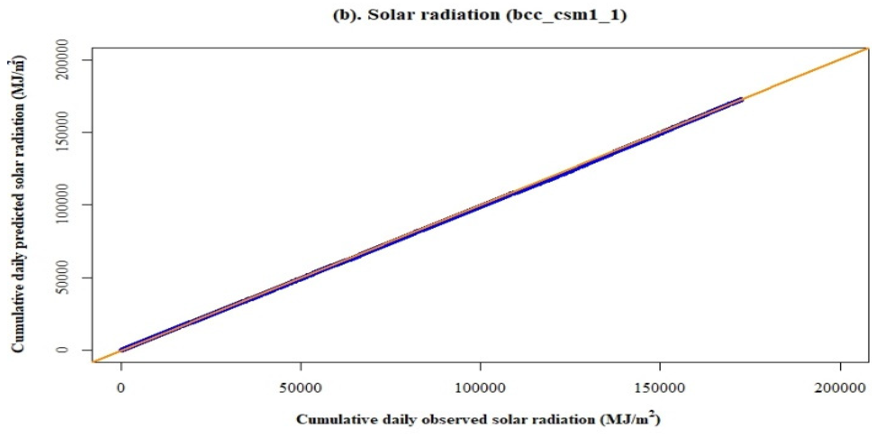
Figure 6 illustrates the relationship between predicted and observed precipitation and solar radiation with the model, bcc_csm1_1. Figure 6a,b describe a consistency between predicted and observed precipitation and solar radiation, respectively.

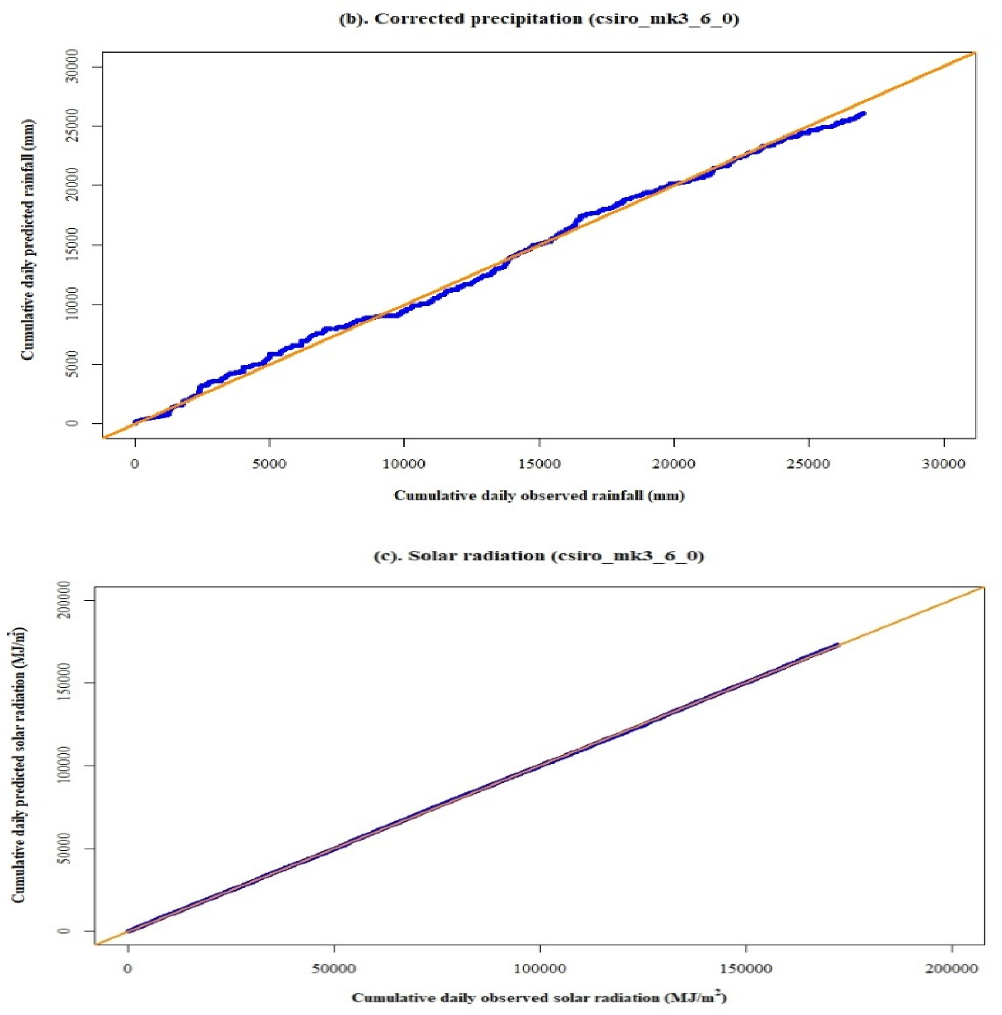
Figure 7 demonstrates the relationship between observed and predicted precipitation by the model, csiro_mk3_6_0. Figure 7a shows the biases in precipitation plot due to the change in slope between predicted and observed data. This inconsistency was removed by dividing the cumulative daily predicted with the slope of 1.13. Thus, Figure 7b was plotted after the correction of predicted precipitation. However, Figure 7c represented no change in proportionality between observed and predicted solar radiation.

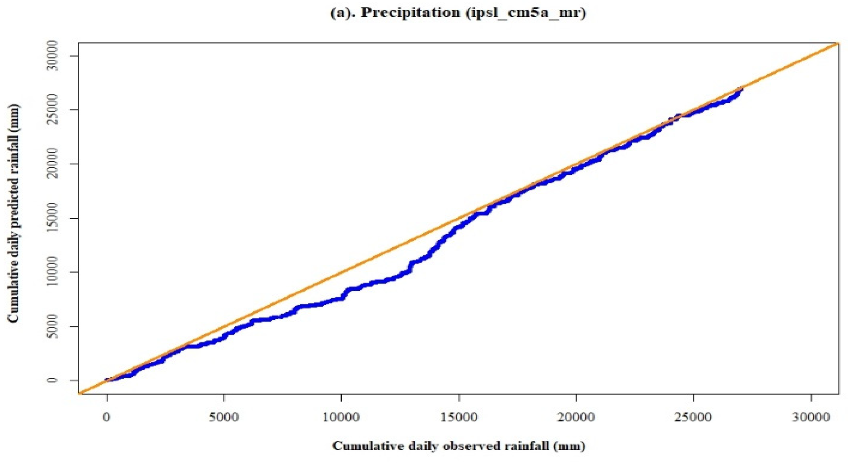
Figure 8a,b illustrate the consistency between observed and predicted precipitation and solar radiation data for the model, ipsl_cm5a_mr. During the baseline period (1980–2004), the proportionality between observed and predicted data for both the variables, precipitation, and solar radiation, was found unchanged. Therefore, it represents no break in the slope between both the variables.

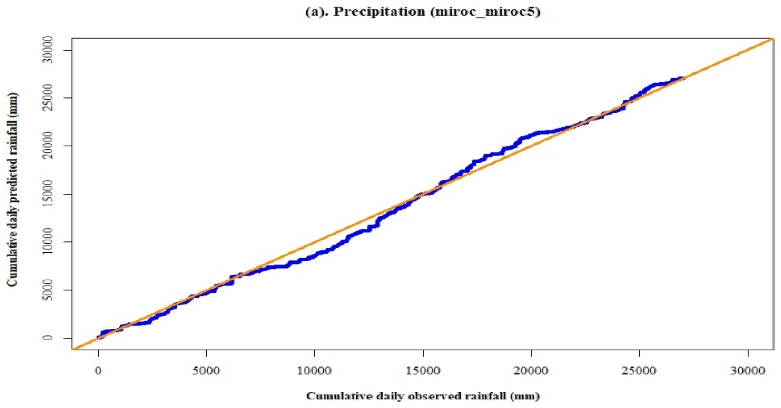
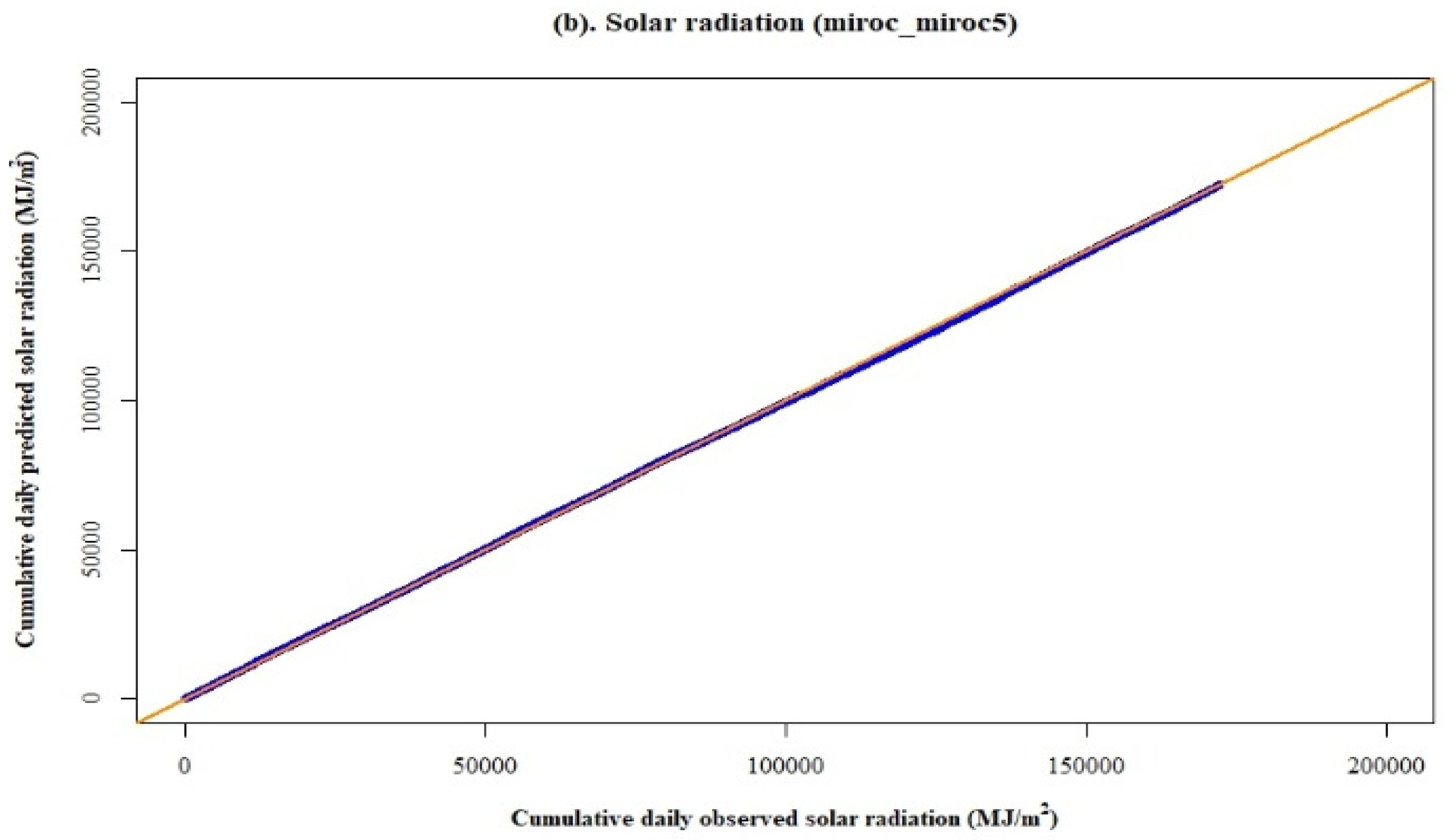
Figure 9a,b show the relationship between observed and predicted precipitation and solar radiation data for the model, miroc_miroc5. This model also demonstrates consistency between observed and predicted data for both the variables. Both the double mass curve plots represent the proportionality between observed and predicted data because the slope between them is not changing.

3.6. Projected Climate Change during 2020–2059

3.6.1. Precipitation

The projected change in rainfall during 2020–2059, from the baseline period (1980–2004) with four climate change scenarios, RCP 2.6, RCP 4.5, RCP 6.0, and RCP 8.5, are shown in Figure 10. Figure 10a (RCP 2.6) illustrates a significant increase in rainfall during monsoon season for all 10 years of the interval from 2020 to 2059. However, there was no defined increase or decrease in precipitation for each decade interval. Moreover, 2050–2059 showed an overall increase in precipitation in the monsoon season, The change in precipitation from the baseline period (1980–2004) for RCP 4.5 (Figure 10b) shows a maximum increase in rainfall that occurred between the months of May and September. The highest change in rainfall of 77.02 mm was observed in the month of September for the period of 2020–2029. Winter season exhibited no significant increase or decrease in the rainfall.

In addition to the abovementioned, RCP 6.0 (Figure 10c) presents the maximum increase in precipitation of 65 mm and 57 mm in the months of August (during 2040–2049) and September (during 2050–2059), respectively. In contrast to RCP 2.6 and RCP 4.5, an increase in rainfall by 21 mm from baseline was observed in the months of October and November, during 2050–2059. The change in precipitation for the scenario RCP 8.5, also showed the similar variability in precipitation change, which increases in the monsoon season (June–September) for all the 10 years of interval (Figure 6d).

3.6.2. Maximum Temperature

The projected change in maximum temperature from baseline period (1980– 2004) for the low greenhouse gases emission scenario, RCP. 2.6, shows that temperature is expected to increase very high up to 3 °C during 2050–2059 in the month of June. A constant increase in maximum temperature can be envisaged from Figure 11b. The maximum temperature will increase up to 1.14 °C/month and 1.94 °C/month during the winter of 2020 and 2059, respectively, with RCP 4.5. Similar to RCP 2.6, this scenario has also revealed less increase in maximum temperature during monsoon season. The highest increase of 0.94 °C was observed in the month of August during 2050–2059.

The scenario RCP 6.0 observed less increase in maximum temperature during winter season compared to RCP 4.5 (Figure 11c). During the winter of 2020–2029 and 2050–2059, the highest increase in maximum temperature was predicted to be 1 °C/month and 1.79 °C/month, respectively. Monsoon season during the years of 2020–2029 and 2050–2059 will expect the change of 0.29–0.46 °C/month and 0.79–0.88 °C/month, respectively. In addition, the worst case scenario, RCP 8.5, is expected to increase the maximum temperature during the winter of 2020–2029 and 2050–2059 by 1.58 °C/month and 2.38 °C/month, respectively. Similar to other scenarios, May and June will be hottest months all the years from 2020–2059. The maximum temperature will rise up to 3.20 °C and 3.38 °C in the months of May and June, respectively, during 2050–2059. Figure 11d also exhibits that the monsoon season will have a very high increase in maximum temperature with RCP 8.5 compared to other scenarios. The highest change from the baseline period (1980–2004) will reach up to 1.17 °C/month during 2050–2059.

3.6.3. Minimum Temperature

A continuous increase in minimum temperature for most of the months was observed with every 10 years of the interval during 2020–2059. The highest increase of 0.89 °C/month and 1.55 °C/month were predicted for winter season during 2020–2029 and 2050–2059, respectively, with RCP 2.6 (Figure 12a). Monsoon season (June–September) will expect a minimum change of 0.39 °C in the month of September during 2020–2029, while the maximum change of 1.36 °C is expected to occur in the month of June during 2050–2059. Moreover, Figure 12b shows projection change in minimum temperature with the intermediate scenario, RCP 4.5. The highest increase in minimum temperature of 2.20 °C during the winter season was observed in the month of November from 2050 to 2059. Further, the month of June in monsoon season is expected to observe the largest increase of 0.98 °C and 1.87 °C during 2020–2029 and 2050–2059, respectively. Under the scenario, RCP 6.0, the month of November will again expect the highest increase in minimum temperature of 1.03 °C and 1.72 °C during 2020–2029 and 2050–2059, respectively. All months in monsoon season, except June (1.07 °C), will experience a relatively smaller variation in minimum temperature between (0.46–0.52) °C/month, during 2020–2029. However, the projection change in minimum temperature will increase up to 2.15 °C and 1.23 °C in the month of June and September, respectively, during 200–2059. In addition to that, the pattern of change in minimum temperature with the worst case scenario, RCP 8.5 (Figure 12d), is similar to other scenarios. The month of November will experience the highest rise in minimum temperature of 1.31 °C and 2.45 °C during 2020–2029 and 2050–2059, respectively. The smallest change of 0.79 °C can be seen from Figure 12d in the month of December for 2020–2029. In the monsoon season, the month of July will expect very little change of 0.49 °C, while June will observe the maximum rise of 1.67 °C, during 2020–2029. Further, the highest increase in minimum temperature of 2.34 °C can be seen from Figure 12d in the month of June during 2050–2059.

3.6.4. Solar Radiation

Figure 13a shows the change in solar radiation with RCP 2.6. The maximum decrease in the shortwave radiation of 1.15 MJ/m² in the month of May was observed from 2050 to 2059. Further, the intermediate scenario, RCP 4.5, will cause the largest decrease of 0.35 MJ/m² during 2050–2059 for two months in the winter season, November and December (Figure 13b). No significant change of increase or decrease can be seen in the monsoon season from 2020 to 2059. Figure 13c shows the change in solar radiation with RCP 6.0, and provides a better significant trend from 2020 to 2059, compared to the other two previous scenarios. This scenario has shown less decrease in radiation in the winter season compared to RCP 4.5. In the monsoon season, June has shown the minimal increase of 0.04 MJ/m² and 0.12 MJ/m² during 2020–2029 and 2030–2039, respectively, and a maximum decrease of 1.19 MJ/m² during 2050–2059.

The worst case scenario, RCP 8.5, shows a large change in solar radiation with each decade from 2020 to 2059. This scenario also establishes the fact that the worst case scenario will hamper the incoming solar radiation very critically. In the winter season, the maximum decrease will take the place of 0.60 MJ/m²/month and 0.96 MJ/m²/month during 2020–2029 and 2050–2059, respectively. The month of June, in monsoon season, will experience the highest decrease of 2.82 MJ/m². An average decrease for all months in monsoon season can be seen around 1.30 MJ/m²/month and 1.49 MJ/m²/month during 2020–2029 and 2050–2059, respectively.

4. Discussion

The results obtained in this study suggest variability in climatic factors will affect the agricultural production and water requirements for those productions [12,18]. Variability in rainfall may cause flooding conditions, as currently, this situation also exists in major agricultural states in India, while change in temperature will lead to affect the crop production by altering the phenological days [33,34].

The analysis of mean absolute errors showed that the magnitude of errors for maximum and minimum temperature were lower than precipitation and solar radiation. Further, the magnitude of mean absolute error for minimum temperature was smaller than the error in maximum temperature. The three models exhibit the marginally smaller standard deviation for simulated precipitation compared to the observed standard deviation. The minimum errors and high correlation between observed and predicted climate data reveals large confidence on the climate data for the use of agricultural modeling purpose and effectively applying for agricultural management policies [35,36]. The trend for precipitation is unpredictable, which may cause an increase or decrease in water requirements as well as affecting farming practices [37,38]. However, a significant increasing trend for temperature indicates large water demand for crop production, caused due to high evapotranspiration [39,40]. Further, decreasing trend of solar radiation reduces the assimilation of dry matter in plants, by affecting metabolic growth [12,41,42].

It can be inferred from the projected climate that rainfall may fluctuate from a very high to a very low level. This is a significant result—this variability in the precipitation due to the uncertainty in monsoon rainfall causes floods and droughts in the state of Bihar [43]. The range of increase in maximum temperature during monsoon season was very low compared to other seasons (Figure 11a). Since frequent rainfall and appearance of cloudy skies commence in the month of July, the temperature starts decreasing from this month [44,45]. Due to the late arrival of monsoon in June, the change in T_max was found to be at peak during this month [46,47]. A non-uniform shift for each decade in shortwave radiation is caused by increase in greenhouse gases concentration which holds the radiation in the atmosphere from reaching the earth’s surface [45,46,47]. Therefore, in summary, the three major understandings of our study are:

1. The results show predominant climate change patterns affecting rice production in the state of Bihar, and if nothing changes, the farming practices will be unsustainable.

2. The study also provided information on how and which production practices may be changed/shifted to accommodate the climate change patterns in order to maximize the rice production and effectively utilize climatic variables.

3. The results would be used to educate the farmers to change their production practices. It can also help to introduce new policy and justification for incentives to the farmers for adopting the change.

5. Conclusions

This study was carried out to project the variability in future climate change, to establish the relationship between historical observed and model-simulated data, to determine the future climate trends from all the four selected GCMs, and to project a total climate change from ensemble mean of all the GCMs. The analysis of variability in precipitation and temperature explains the reason of flood or drought appearing at the intermittent interval, during monsoon season. Due to the cloudiness during monsoon season and variability in precipitation, the correlation for precipitation and solar radiation was observed low, and the deviation between observed and simulated data for these two factors was also found considerably higher compared to the maximum and minimum temperature. Trend analysis and projection change of climatic factors revealed how the crop production and water requirement will become affected in future. A significant increasing trend for maximum and minimum temperature will lead the agricultural practices to require more water, and both of these factors including decrease in solar radiation will cause reduction in phenological days. The results of this study have potential for policy change for the rice production practices in Bihar, India. This study shows that climate variability (temperature, precipitation, etc.) is predominant and the rice production practices are unsustainable if no change in practices or policy are adopted. Based on temperature and precipitation, the crop growth period may be slightly changed (advanced) in order to capture and utilize most of the natural precipitation. The local authorities may help in making people understand the need for these changes and their implications, and perhaps incentivize farmers who adopt these practices for taking the risk of yield uncertainty.

References

1. Awal, R.; Bayabil, H.K.; Fares, A. Analysis of Potential Future Climate and Climate Extremes in the Brazos Headwaters Basin, Texas. Water 2016, 8, 603. [Google Scholar] [CrossRef] [Green Version]
2. Kumar, R.; Gautam, H.R. Climate Change and Its Impact on Agricultural Productivity in India. J. Climatol. Weather Forecast. 2014, 2. [Google Scholar] [CrossRef] [Green Version]
3. Jena, P.; Azad, S.; Rajeevan, M.N. CMIP5 Projected Changes in the Annual Cycle of Indian Monsoon Rainfall. Climate 2016, 4, 14. [Google Scholar] [CrossRef] [Green Version]
4. Intergovernmental Panel on Climate Change (IPCC) Working Group II. Climate Change 2014: Impacts, Adaptation, and Vulnerability. Part B: Regional Aspects, Polar Regions; Cambridge University Press: New York, NY, USA, 2014; pp. 1567–1612. [Google Scholar] [CrossRef]
5. Gehne, M.; Hamill, T.M.; Kiladis, G.N.; Trenberth, K.E. Comparison of Global Precipitation Estimates across a Range of Temporal and Spatial Scales. J. Clim. 2016, 29, 7773–7795. [Google Scholar] [CrossRef]
6. Bosello, F.; Zhang, J. Assessing Climate Change Impacts: Agriculture; FEEM Working Paper No. 94.05; CMCC Research Paper No. 2; Elsevier: New York, NY, USA, 2005; Available online: https://ssrn.com/abstract=771245 (accessed on 31 May 2021).
7. Meinshausen, M.; Smith, S.J.; Calvin, K.; Daniel, J.S.; Kainuma, M.L.T.; Lamarque, J.; Matsumoto, K.; Montzka, S.A.; Raper, S.C.B.; Riahi, K.; et al. The RCP Greenhouse Gas Concentrations and Their Extensions from 1765 to 2300. Clim. Chang. 2011, 109, 213–241. [Google Scholar] [CrossRef] [Green Version]
8. Van Vuuren, D.P.; Edmonds, J.; Kainuma, M.; Riahi, K.; Thomson, A.; Hibbard, K.; Hurtt, G.C.; Kram, T.; Krey, V.; Lamarque, J.F.; et al. The Representative Concentration Pathways: An Overview. Clim. Chang. 2011, 109, 5–31. [Google Scholar] [CrossRef]
9. Budhathoki, N.K.; Zander, K.K. Nepalese Farmers’ Climate Change Perceptions, Reality and Farming Strategies. Clim. Dev. 2020, 12, 204–215. [Google Scholar] [CrossRef]
10. Dasgupta, P.; Morton, J.F.; Dodman, D.; Karapinar, B.; Meza, F.; Rivera-Ferre, M.G.; Toure Sarr, A.; Vincent, K.E. Rural areas. In Climate Change 2014: Impacts, Adaptation, and Vulnerability; Part A: Global andSectoral Aspects; Contribution of Working Group II to the Fifth Assessment Report of the Intergovernmental Panel on Climate Change; Field, C.B., Barros, V.R., Dokken, D.J., Mach, K.J., Mastrandrea, M.D., Bilir, T.E., Chatterjee, M., Ebi, K.L., Estrada, Y.O., Genova, R.C., et al., Eds.; Cambridge University Press: Cambridge, UK; New York, NY, USA, 2014; pp. 613–657. [Google Scholar]
11. Fróna, D.; Szenderák, J.; Harangi-Rákos, M. The Challenge of Feeding the World. Sustainability 2019, 11, 5816. [Google Scholar] [CrossRef] [Green Version]
12. Jha, R.K.; Kalita, P.K.; Cooke, R.A.; Kumar, P.; Davidson, P.C.; Jat, R. Predicting the Water Requirement for Rice Production as Affected by Projected Climate Change in Bihar, India. Water 2020, 12, 3312. [Google Scholar] [CrossRef]
13. Raza, A.; Razzaq, A.; Mehmood, S.S.; Zou, X.; Zhang, X.; Lv, Y.; Xu, J. Impact of Climate Change on Crops Adaptation and Strategies to Tackle Its Outcome: A Review. Plants 2019, 8, 34. [Google Scholar] [CrossRef] [PubMed] [Green Version]
14. Aryal, J.P.; Sapkota, T.B.; Khurana, R.; Khatri-Chhetri, A.; Rahut, D.B.; Jat, M.L. Climate Change and Agriculture in South Asia: Adaptation Options in Smallholder Production Systems. Environ. Dev. Sustain. 2020, 22, 5045–5075. [Google Scholar] [CrossRef] [Green Version]
15. Rojas-Downing, M.M.; Nejadhashemi, A.P.; Harrigan, T.; Woznicki, S.A. Climate Change and Livestock: Impacts, Adaptation, and Mitigation. Clim. Risk Manag. 2017, 16, 145–163. [Google Scholar] [CrossRef]
16. Arora, N.K. Impact of Climate Change on Agriculture Production and Its Sustainable Solutions. Environ. Sustain. 2019, 2, 95–96. [Google Scholar] [CrossRef] [Green Version]
17. Mall, R.K.; Singh, R.; Gupta, A.; Srinivasan, G.; Rathore, L.S. Impact of Climate Change on Indian Agriculture: A Review. Clim. Chang. 2006, 78, 445–478. [Google Scholar] [CrossRef] [Green Version]
18. Tesfaye, K.; Aggarwal, P.K.; Mequanint, F.; Shirsath, P.B.; Stirling, C.M.; Khatri-Chhetri, A.; Rahut, D.B. Climate Variability and Change in Bihar, India: Challenges and Opportunities for Sustainable Crop Production. Sustainability 2017, 9, 1998. [Google Scholar] [CrossRef] [Green Version]
19. Joshi, P.K.; Roy, D.; Sonkar, V.; Tripathi, G. Technologies for Maize, Wheat, Rice and Pulses in Marginal Districts of Bihar and Odisha. In Technological and Institutional Innovations for Marginalized Smallholders in Agricultural Development; Gatzweiler, F.W., von Braun, J., Eds.; Springer International Publishing: Cham, Switzerland, 2016; pp. 323–367. [Google Scholar] [CrossRef] [Green Version]
20. High-Resolution and Bias-Corrected CMIP5 Projections for Climate Change Impact Assessments|Scientific Data. Available online: https://www.nature.com/articles/s41597-019-0343-8 (accessed on 31 May 2021).
21. Tang, X.; Zhang, J.; Gao, C.; Ruben, G.B.; Wang, G. Assessing the Uncertainties of Four Precipitation Products for Swat Modeling in Mekong River Basin. Remote Sens. 2019, 11, 304. [Google Scholar] [CrossRef] [Green Version]
22. Chisanga, C.; Phiri, E.; Chinene, V.R.N. Statistical Bias Correction of Fifth Coupled Model Intercomparison Project Data from the CGIAR Research Program on Climate Change, Agriculture and Food Security-Climate Portal for Mount Makulu, Zambia. Br. J. Appl. Sci. Technol. 2017, 21, 1–16. [Google Scholar] [CrossRef] [Green Version]
23. Yaghoubi, F.; Bannayan, M.; Asadi, G.-A. Performance of Predicted Evapotranspiration and Yield of Rainfed Wheat in the Northeast Iran Using Gridded AgMERRA Weather Data. Int. J. Biometeorol. 2020, 64, 1519–1537. [Google Scholar] [CrossRef]
24. Mehrotra, R.; Sharma, A. A Multivariate Quantile-Matching Bias Correction Approach with Auto- and Cross-Dependence across Multiple Time Scales: Implications for Downscaling. J. Clim. 2016, 29, 3519–3539. [Google Scholar] [CrossRef]
25. Banacos, P.C. Eastern Region Technical Attachment Box and Whisker Plots for Local Climate Datasets: Interpretation and Creation Using Excel 2007/2010. Interpret. J. Bible Theol. 2011, 1, 2–20. [Google Scholar]
26. Chai, T.; Draxler, R.R. Root Mean Square Error (RMSE) or Mean Absolute Error (MAE)?—Arguments against Avoiding RMSE in the Literature. Geosci. Model Dev. 2014, 7, 1247–1250. [Google Scholar] [CrossRef] [Green Version]
27. Taylor, K.E. Summarizing Multiple Aspects of Model Performance in a Single Diagram. J. Geophys. Res. Atmos. 2001, 106, 7183–7192. [Google Scholar] [CrossRef]
28. Mann, H.B. Non-Parametric Test against Trend. Econometrica 1945, 13, 245–259. [Google Scholar] [CrossRef]
29. Kendall, M.G. Rank Correlation Methods, 4th ed.; Charles Griffin: London, UK, 1975; p. 272. [Google Scholar]
30. Fraile, R. On the Statistical Analysis of Series of Observations: By R. Sneyers. World Meteorological Organization, Geneva, Technical Note N° 143, 1990, U.D.C. 551.501.45, 192 p. Atmos. Res. 1993, 29, 274. [Google Scholar] [CrossRef]
31. Karpouzos, D.; Kavalieratou, S.; Babajimopoulos, C. Trend Analysis of Precipitation Data in Pieria Region (Greece). Eur. Water 2010, 30, 30–40. [Google Scholar]
32. Sen, P.K. Estimates of the Regression Coefficient Based on Kendall’s Tau. J. Am. Stat. Assoc. 1968, 63, 1379–1389. [Google Scholar] [CrossRef]
33. Mahmood, R. Impacts of Air Temperature Variations on the Boro Rice Phenology in Bangladesh: Implications for Irrigation Requirements. Agric. For. Meteorol. 1997, 84, 233–247. [Google Scholar] [CrossRef]
34. Sharma, H.L.; Kumar, R. Simulating Phenology and Yield of Rice Using Ceres- Rice Model in North Western Himalayas. Indian J. Plant Physiol. 2005, 10, 280–282. [Google Scholar]
35. Shi, W.; Tao, F.; Zhang, Z. A Review on Statistical Models for Identifying Climate Contributions to Crop Yields. J. Geogr. Sci. 2013, 23, 567–576. [Google Scholar] [CrossRef]
36. Asare-Nuamah, P.; Botchway, E. Understanding Climate Variability and Change: Analysis of Temperature and Rainfall across Agroecological Zones in Ghana. Heliyon 2019, 5, e02654. [Google Scholar] [CrossRef] [PubMed] [Green Version]
37. Joshi, N.; Maharjan, K.; Piya, L. Effect of Climate Variables on Yield of Major Food-Crops in Nepal: A Time-Series Analysis. J. Contemp. Indian Stud. Space Soc. 2011, 1, 19–26. [Google Scholar] [CrossRef] [Green Version]
38. Kelkar, S.; Kulkarni, A.; KUNDETI, K. Impact of Climate Variability and Change on Crop Production in Maharashtra, India. Curr. Sci. 2020, 118, 1235–1245. [Google Scholar] [CrossRef]
39. Ali, M.; Adham, A.K.M. Impact of Climate Change on Crop Water Demand and Its Implication on Water Resources Planning: Bangladesh Perspective. J. Agrometeorol. 2007, 9, 20–25. [Google Scholar]
40. Rao, V.; Subbarao, A.; Rao, G.; Satyanarayana, T.; Narayanan, M.; Venkateshwarlu, B. Impact of Climate Change on Crop Water Requirements and Adaptation Strategies. In Challenges and Opportunities in Agrometeorology; Springer: Berlin/Heidelberg, Germany, 2011; pp. 311–319. [Google Scholar] [CrossRef]
41. Nieuwenhuizen, W.N. The Effects of Solar Radiation and Nutrient Solution Temperature on the Uptake of Oxygen by Submerged Roots of Mature Tomato Plants. Plant Soil 1983, 70, 353–366. [Google Scholar] [CrossRef]
42. Ferrante, A.; Mariani, L. Agronomic Management for Enhancing Plant Tolerance to Abiotic Stresses: High and Low Values of Temperature, Light Intensity, and Relative Humidity. Horticulturae 2018, 4, 21. [Google Scholar] [CrossRef] [Green Version]
43. Praveen, B.; Talukdar, S.; Mahato, S.; Mondal, J.; Sharma, P.; Islam, A.R.M.T.; Rahman, A. Analyzing Trend and Forecasting of Rainfall Changes in India Using Non-Parametrical and Machine Learning Approaches. Sci. Rep. 2020, 10, 10342. [Google Scholar] [CrossRef]
44. Naidu, C.V.; Durgalakshmi, K.; Krishna, K.; Rao, S.; Satyanarayana, G.; Lakshminarayana, P.; Rao, L. Is Summer Monsoon Rainfall Decreasing over India in the Global Warming Era? J. Geophys. Res. 2009, 114. [Google Scholar] [CrossRef] [Green Version]
45. Gajbhiye, S.; Meshram, C.; Mirabbasi, R.; Sharma, S. Trend Analysis of Rainfall Time Series for Sindh River Basin in India. Theor. Appl. Climatol. 2015, 125, 593–608. [Google Scholar] [CrossRef]
46. Rajeevan, M.; Unnikrishnan, C.K.; Bhate, J.; Niranjan Kumar, K.; Sreekala, P.P. Northeast Monsoon over India: Variability and Prediction. Meteorol. Appl. 2012, 19, 226–236. [Google Scholar] [CrossRef]
47. Jaswal, A.K.; Rao, P.C.S.; Singh, V. Climatology and Trends of Summer High Temperature Days in India during 1969–2013. J. Earth Syst. Sci. 2015, 124, 1–15. [Google Scholar] [CrossRef] [Green Version]
Figure 1. Topography map of the study area, Bihar, located in India, showing elevation.
Climate 09 00111 g001
Figure 2. Flowchart for obtaining and processing of the climate data.
Climate 09 00111 g002
Figure 3. Box and whisker plot of the ensemble mean of climate simulated data from all four selected models for the baseline period (1980–2004).
Climate 09 00111 g003
Figure 4. Comparison of mean absolute error for climatic factors with all the four global climate models.
Climate 09 00111 g004
Figure 5. Taylor diagram exhibiting statistical comparisons of observation and four global climate models predicted data for (a) precipitation, (b) maximum temperature, (c) minimum temperature, and (d) solar radiation.
Climate 09 00111 g005
Figure 6. Double mass curve plots for the precipitation and solar radiation data by the model, bcc_csm1_1, for the baseline period (1980–2004).
Climate 09 00111 g006aClimate 09 00111 g006b
Figure 7. Double mass curve plots for the precipitation (a,b) and solar radiation data (c) by the model, csiro_mk3_6_0, for the baseline period (1980–2004).
Climate 09 00111 g007aClimate 09 00111 g007b
Figure 8. Double mass curve plots for the precipitation and solar radiation data by the model, ipsl_cm5a_mr, for the baseline period (1980–2004).
Climate 09 00111 g008aClimate 09 00111 g008b
Figure 9. Double mass curve plots for the precipitation and solar radiation data by the model, miroc_miroc5, for the baseline period (1980–2004).
Climate 09 00111 g009aClimate 09 00111 g009b
Figure 10. Projection of precipitation change for 10 years of the interval during 2020–2060 for (a) RCP 2.6, (b) RCP 4.5, (c) RCP 6.0, and (d) RCP 8.5.
Climate 09 00111 g010aClimate 09 00111 g010b
Figure 11. Projection of maximum temperature change for 10 years of the interval during 2020–2060 for (a) RCP 2.6, (b) RCP 4.5, (c) RCP 6.0, and (d) RCP 8.5.
Climate 09 00111 g011aClimate 09 00111 g011b
Figure 12. Projection of minimum temperature change for 10 years of the interval during 2020–2060 for (a) RCP 2.6, (b) RCP 4.5, (c) RCP 6.0, and (d) RCP 8.5.
Climate 09 00111 g012aClimate 09 00111 g012b
Figure 13. Projection of solar radiation change for 10 years of interval during 2020–2060 for (a) RCP 2.6, (b) RCP 4.5, (c) RCP 6.0, and (d) RCP 8.5.
Climate 09 00111 g013aClimate 09 00111 g013b