A Simple Theoretical Model for Lags and Asymmetries of Surface Temperature

Abstract

Here, we study three fundamental climatic phenomena: The seasonal lag, the diurnal lag, and the asymmetry of daily temperature variation. We write a nonlinear ODE based on an energy balance for surface temperature and humidity. The model focuses on small regions of the Earth’s surface; it reproduces the three phenomena with a reasonable accuracy if a few parameters are chosen according to the climatic type of the regions. The plots in this manuscript compare real climatic data with numerical solutions of the model we propose. The model takes into account the doubly periodic forcing of the solar radiation (annual and daily), IR radiation, the existence of thermodynamic bodies with different thermal inertia (land and oceans), and the effect of humidity on the thermal inertia of the air. We write the equations using astronomical parameters with the possibility of applications to exoplanets in mind. We conclude this article investigating the evolution of temperatures in Catania and Sydney if the Earth was on an orbit around the Sun with the same mean distance but greater eccentricity.

1. Introduction

The first models in modern climatology date back to the late 1800s, early 1900s [1,2,3]. They were based on a combination of incoming and outgoing radiation and Navier–Stokes equations, since climate is driven by energy balance and motion of fluid masses. Energy balance has however different effects on the surface temperatures on Earth, because each region has different composition and hence different effective thermal inertia. Moreover, average heat exchanges inside the region and between different regions can be very different depending on their composition.

Relying on these ingredients, early meteorologists considered weather forecasting impossible [3]. This is not so obvious when dealing with climatology. In climatology, the evolution of average thermodynamic variables is reasonably not as much influenced by diffusion phenomena [4]. Some local variations of temperature and other thermodynamic variables are due to motion of fluid masses. Excluding systematic effects (caused for example by the rotation of the Earth, the difference between polar and equatorial temperatures, etc.), these type of variations average out in a climatic period of 30–50 years. The systematic effects can be accounted for indirectly, by adapting the parameters. For the reasons above, some climatic phenomena can be investigated including diffusion only as a marginal effect through a compensation in the parameters. This allows one to reproduce many climatic effects considering non-sophisticated models which, despite their simplicity, can be reasonably predictive.

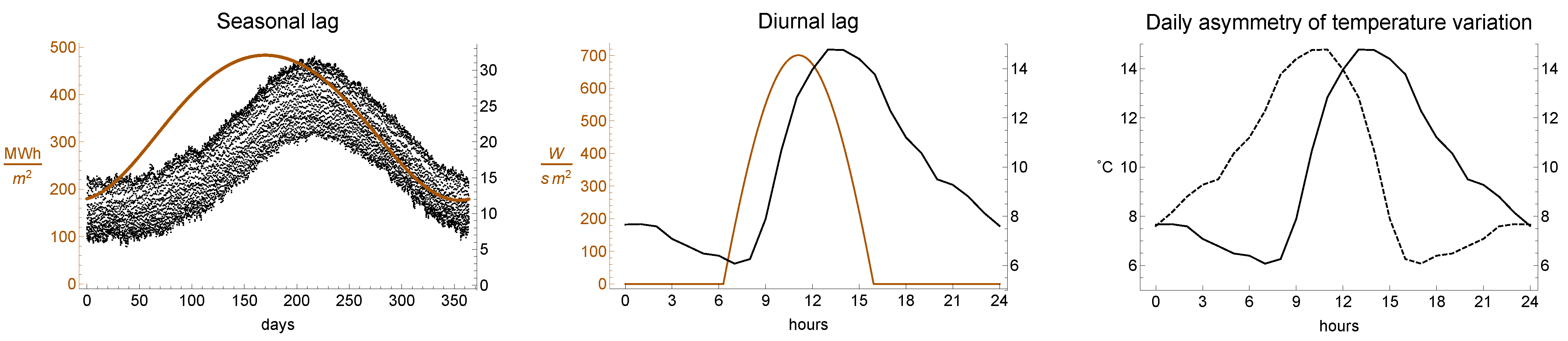
In this article we focus on three main climatic effects. The first phenomenon is called seasonal lag, or lag of seasons. With this name one indicates the well known fact that the warmer days of the year take place a variable number of weeks after the days of maximal solar irradiance. The second phenomenon is the less celebrated phenomenon of diurnal lag, or lag of noons. With this name we indicate the fact that the warmer hours of the day take place from one to a few hours after the moment of strongest solar irradiance. The third phenomenon is the daily asymmetry of temperature variation. With this name we indicate the fact that daily temperatures rise much faster in the morning than they fall in the afternoon. In Figure 1 we graphically represent the three phenomena.

The delays are well known in boundary layer meteorology and play an important role for example in urban climate. What we prove in this manuscript is that the most basic model that displays these three phenomena must necessarily include two thermodynamic bodies (land and ocean) and the humidity. The two thermodynamic bodies and their thermal inertia do provide the two distinct and independent delays, which are very different depending on the climatic zone in which one is performing the investigation. The evolution of air humidity during the day does provide a changing thermal inertia of the air, which in turns creates a difference between the morning raise of temperatures and their afternoon decay.

The ultimate goal of this manuscript is to suggest a model that reproduces the three climatic effects above but also, where possible, provides a realistic evolution of average surface temperatures and humidity. In this manuscript with average temperatures of a region $\mathcal{R}$ we mean the function $\overline{T}:[01/01\mathrm{at}00:00,12/31\mathrm{at}24:00]\to \mathbb{R}$ obtained by averaging the surface temperatures at a chosen day, hour and minute of the years from 1973 to 2020 (48 years) measured at a chosen WMO station inside $\mathcal{R}$. More explicitly

$$\overline{T}(\overline{month},\overline{day},\overline{hour},\overline{min})=\frac{1}{48}\sum _{y=1973}^{2020}T(y,\overline{month},\overline{day},\overline{hour},\overline{min}),$$

(1)

with $T(year,month,day,hour,minute)$ being the temperature at a given UTC time. The same procedure has been used to define the average relative humidity of a region. Nowadays temperatures and humidity datasets are easily available also to non-professional meteorologists. There are about 10,000 WMO station around the world, each of which makes from 5000 to 20,000 measures a year since 1973. This allowed us to compute the averaged functions for temperature and relative humidity with time steps of 1 h, and compare them with simulations.

In this work we operate a number of simplifications that might be reasonable or partially acceptable. For example we do not consider altitude and meridional heat fluxes. To deal with altitude one could not exclude the contribution of neighbouring cooler regions; also meridional fluxes have a stationary component. Even worse, stationary heats fluxes such as the Gulf Stream can be accounted for only with a detailed inclusion of global geomorphology. We also disregard synoptic storms and eddy-diffusion [5], effects that could give a sensible deviation the model. This is stated to make it clear that our intent is not to give an accurate predictive system, but to provide a simple model that supports and justifies the three climatic phenomena described above.

In [6] the authors discuss a very simple mathematical model to explain the phenomenon of lag of seasons. Elementary mathematics proves that the long-term solution to the equation

$$\dot{T}\left(t\right)=(-\lambda T\left(t\right)+\mu )+(acos\left(\omega t\right)+b)$$

(2)

is

$$\frac{\mu +b}{\lambda }+\frac{a}{\sqrt{{\lambda }^2+{\omega }^2}}cos\left(\omega (t-\tau )\right),$$

(3)

where $\tau =\phi /\omega$ and $\phi =arg(\lambda +i\omega )$. Equation (2) is an extremely basic model for the evolution of temperature T of a region $\mathcal{R}$ on the surface of a planet. In this model T is the temperature of $\mathcal{R}$. The term $-\lambda T+\mu$ is a linearisation of the outgoing radiation from $\mathcal{R}$, while the forcing term $acos\left(\omega t\right)+b$ models the solar irradiance absorbed by $\mathcal{R}$, and $\omega$ is related to the revolution of Earth. It clearly follows from (3) that the temperature T has maxima and minima delayed with respect to the maxima and minima of solar irradiance, and the lag of these extremes $\tau$ corresponds to the lag of seasons.

An approach that takes into consideration only Sun’s irradiation and Fourier’s law cannot reproduce the three phenomena. The simple introduction of a forcing term containing two frequencies (daily rotation and annual revolution) is not enough to give realistic predictions of both lags (noon and seasons) [7]. To make such predictions one must increase the number of degrees of freedom. In fact, the first model whose solutions correctly predict both effects uses at least two different thermodynamic bodies with different thermal inertia, which correspond to a system with two degrees of freedom [8]. A quantitative analysis of the two lags is performed in Appendix A. The asymmetry of temperatures is a further effect, and to be reproduced it requires the introduction of one more degree of freedom, that models the evolution of the absolute humidity of the air.

In the literature, climatic models can be roughly divided into two categories: global circulation models (GCMs) [4] and energy balance models (EBMs) [6]. In GCMs land, oceans, and atmosphere are discretised into cells, and flows and energy transfer among cells are integrated over time; in EBMs the evolution of temperature is computed through low-dimensional systems, and the investigation is typically local or mediated along a parallel. GCMs can predict climate more accurately, but they require great effort to acquire data, to set up the simulation, and need large computing capacities. EBMs are possibly less accurate but require much less computational resources. EBMs have often been used to investigate climate under hypothetical variations of orbital and environmental parameters [9,10]. Our work belongs to this second class of models. Our model could be used to investigate possible climate changes on Earth (e.g., greenhouse effect) and climate habitability of exoplanets in specific parts of their surface. In particular, at difference from classical one-dimensional EBMs [11], our approach is applicable when the revolution period and the rotation period are in 1:1 resonance (tidal locking) or other low-order resonance.

The outline of the work is the following. In Section 2 we give some geometric definitions and we write explicitly the expression of solar rays inclination. In Section 3 we recall the general laws of heat exchange and evaporation, and we write the evolution equations for temperature and humidity of a region in a generic planet. In Section 4 we numerically solve the equations for various regions on Earth, showing that our model well describes different types of climates (according to the Köppen climate classification [12]) and reproduces the three climatic effects. In Section 5 we discuss the daily and seasonal lags, and compare simulated and measured ones. In Section 6, we discuss the results and indicate possible improvements and applications of the model.

2. The Geometry of Solar Radiation

The motion and orientation in space of a region $\mathcal{R}$ on the surface of a planet is in good approximation due to the composition of the Keplerian revolution of the planet around its star and the rotation of the planet around its axis. The combination of such motions determines intensity and angle of the solar radiation responsible for the heating of the region. Disregarding all possible perturbations to this setting, the power of incoming solar radiation in $\mathcal{R}$ is hence completely determined by its exposition on the planet and the position of the planet in space.

2.1. Geometrical Definitions

In our model the planet is assumed to be an ellipsoid. Its center of mass, following Kepler’s laws, revolves around the Sun along an ellipse belonging to a plane called ecliptic plane. The planet also rotates uniformly around an invariable axis which makes a fixed angle $\gamma$, called obliquity, with respect to the normal of the ecliptic plane. The two points of the planet whose movement is not due to rotation are called North and South poles, which are posed respectively at latitude $+90$ and $-90$ degrees (or $\pi /2$ and $-\pi /2$ radians). The tropics are the two circles of points that have latitude $\pm \gamma$. We plan to describe the evolution of temperature in a certain region of the planet situated at a fixed latitude $\phi$ and longitude $\psi$.

Astronomically speaking, significant times are those in which the Sun rays have global and local minimal (or maximal) angle from the zenith, and they are called solar solstices and solar noon. Climatically speaking, significant instants are those in which the temperature has global and local maximum (or minimum).

Definition 1.

The thermal solstices are the global extremes (maximum and minimum) of the temperature in a zone of the planet during the year. The thermal noon is the moment in which the temperature is at a local maximum.

It is an empirical climatic fact that the thermal solstice and thermal noon are delayed with respect to the respective solar solstice and noon. Such delays are called seasonal lag and diurnal lag.

2.2. Inclination of Solar Rays

Let us consider a planet P rotating around its sun S, and let $\overrightarrow{e_1},\overrightarrow{e_2},\overrightarrow{e_3}$ be an orthonormal reference frame fixed with respect to the stars. The vector $\overrightarrow{e_1}$ is parallel to the semi-major axes of the Keplerian orbit of P and is directed from S to P when P is at the perihelion; the vector $\overrightarrow{e_3}$ is normal to the ecliptic plane and is such that the rotation of P around the sun is counterclockwise; the vector $\overrightarrow{e_2}=\overrightarrow{e_3}\times \overrightarrow{e_1}$ completes the frame and is parallel to the semi-minor axis.

Following the classical description of Keplerian motions, and supposing that at time $t_0=0$ the planet P is located at a certain angle ${\vartheta }_0$ along the orbit, the position of P with respect to the sun is given in polar coordinates by the formulas

$$\rho \left(t\right)=\frac{a(1-e^2)}{1+ecos\left(\vartheta \right(t\left)\right)},\dot{\vartheta }\left(t\right)=\frac{2\pi }{Y{\sqrt{1-e^2}}^3}{(1+ecos\left(\vartheta \left(t\right)\right))}^2,\vartheta \left(0\right)={\vartheta }_0$$

(4)

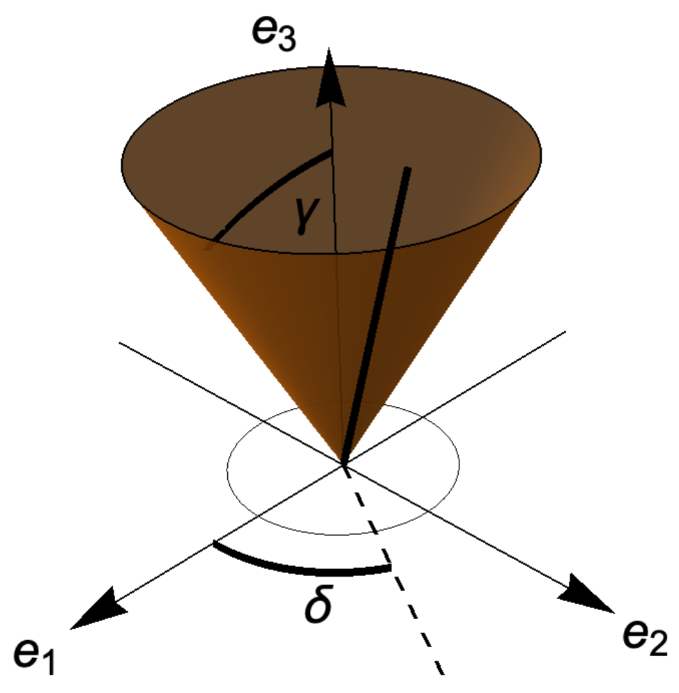
where e is the eccentricity, a is the length of the semi-major axis of the orbit, and Y is the period of revolution. We also suppose that the planet P rotates with angular velocity $\mathsf{\Omega }=2\pi /D$ around an axis invariable in space (D is the period of one rotation, also called sidereal day). Such invariable axis can be determined by two angles, in fact the axis belongs to the cone that forms an angle $\gamma$ with $\overrightarrow{e_3}$ and its projection on the $\overrightarrow{e_1},\overrightarrow{e_2}$ plane forms an angle $\delta$ with the $\overrightarrow{e_1}$-axis moving counterclockwise (see Figure 2).

It follows that a convenient choice of reference frame $\overrightarrow{f_1},\overrightarrow{f_2},\overrightarrow{f_3}$ attached to the rotating body with $\overrightarrow{f_3}$ parallel to the axis of rotation is

$$\left\{\begin{array}{c}\overrightarrow{f_1}\left(t\right)=(cos\gamma cos\delta cos(\Omega t+{\omega }_0)+sin\delta sin(\Omega t+{\omega }_0))\overrightarrow{e_1}+\hfill \\ +(cos\delta sin(\Omega t+{\omega }_0)-cos\gamma sin\delta cos(\Omega t+{\omega }_0))\overrightarrow{e_2}-sin\gamma cos(\Omega t+{\omega }_0)\overrightarrow{e_3}\hfill \\ \overrightarrow{f_2}\left(t\right)=(sin\delta cos(\Omega t+{\omega }_0)-cos\gamma cos\delta sin(\Omega t+{\omega }_0))\overrightarrow{e_1}+\hfill \\ +(cos\delta cos(\Omega t+{\omega }_0)+cos\gamma sin\delta sin(\Omega t+{\omega }_0))\overrightarrow{e_2}+sin\gamma sin(\Omega t+{\omega }_0)\overrightarrow{e_3}\hfill \\ \overrightarrow{f_3}\left(t\right)=sin\gamma cos\delta \overrightarrow{e_2}-sin\gamma sin\delta \overrightarrow{e_1}+cos\gamma \overrightarrow{e_3}.\hfill \end{array}\right.$$

The reference frame $\overrightarrow{f_1},\overrightarrow{f_2},\overrightarrow{f_3}$ can be computed from $\overrightarrow{e_1},\overrightarrow{e_2},\overrightarrow{e_3}$ composing the rotation matrices $R_z(-\delta )R_y(-\gamma )R_z(\Omega t+{\omega }_0)$, where $R_y(-\gamma )$ is the rotation around the y axis of an angle $-\gamma$ and ${\omega }_0$ is needed to pose a specific meridian at midnight when $t=0$. The unit vector pointing from the planet to the sun is

$$\overrightarrow{d}\left(t\right)=-cos\left(\vartheta \left(t\right)\right)\overrightarrow{e_1}-sin\left(\vartheta \left(t\right)\right)\overrightarrow{e_2}.$$

Since the region $\mathcal{R}$ at latitude $\phi$ and longitude $\psi$ has normal to the surface

$$\overrightarrow{n}\left(t\right)=\frac{R_{e}cos\psi cos\phi \overrightarrow{f_1}\left(t\right)+R_{e}sin\psi cos\phi \overrightarrow{f_2}\left(t\right)+R_{p}sin\phi \overrightarrow{f_3}\left(t\right)}{\sqrt{R_e^2{cos}^2\phi +R_p{sin}^2\phi }},$$

where we take into account the fact that the Earth is an ellipsoid with equatorial radius $R_e$ and polar radius $R_p$, it follows that

$$\begin{array}{cc}\hfill \overrightarrow{n}\left(t\right)·\overrightarrow{d}\left(t\right)=& -R_e\frac{cos\phi sin(\psi +\Omega t+{\omega }_0)sin(\delta +\vartheta \left(t\right))}{\sqrt{R_e^2{cos}^2\phi +R_p{sin}^2\phi }}+\hfill \\ & -R_p\frac{sin\gamma sin\phi cos(\delta +\vartheta (t\left)\right)}{\sqrt{R_e^2{cos}^2\phi +R_p{sin}^2\phi }}-R_e\frac{cos\gamma cos\phi cos(\psi +\Omega t+{\omega }_0)cos(\delta +\vartheta \left(t\right))}{\sqrt{R_e^2{cos}^2\phi +R_p{sin}^2\phi }}.\hfill \end{array}$$

(5)

This scalar product will be used in the following section, when writing the solar irradiance. In 

Table 1. Fundamental astronomical parameters for planet Earth.

e	$0.0167$	Eccentricity of Earth’s orbit
a	$1.496\times {10}^{11}\mathrm{m}$	Average Earth-Sun distance
$\gamma$	$23.437{}^{\circ }$	Earth’s mean obliquity
$\delta$	$12.8219{}^{\circ }$	Angle between solstices and perihelion/aphelion
D	$8.616409\times {10}^4\mathrm{s}$	Period of rotation of the Earth
Y	$3.15569\times {10}^7\mathrm{s}$	Period of revolution of the Earth
$R_e$	6,378,136 m	equatorial radius of the Earth
$R_p$	6,356,751 m	polar radius of the Earth

the values of all parameters for the planet Earth are indicated. In particular ${\vartheta }_0=-3(D/Y)2\pi$ to pose January 1st at $t=0$, and ${\omega }_0={\vartheta }_0-\delta =10(D/Y)2\pi$ to pose Greenwich’s meridian at midnight when $t=0$.

3. The Physics of Heat Transfer

The temperature of a region $\mathcal{R}$ on a planet is the result of a balance between the incoming radiation from the sun, the outgoing radiating energy, latent heats and heat exchanges within the system. We model the heat dynamics of such limited region $\mathcal{R}$ located at a certain latitude $\phi$ and a certain longitude $\psi$. We disregard spatial diffusion and hence we use ordinary differential equations in which time is the independent variable. This is not a reasonable assumption when dealing with meteorology, and it is also climatically unreasonable due to stationary heat flows among regions, such as the meridional heat transport. In this model such systematical contributions can be taken into account slightly modifying the parameters which model the incoming and outgoing fluxes (reflectance and absorbance). All other effects will average out because we do compare numerical solutions of the system with average temperatures and humidity of a region. For these reasons we suppose that the region $\mathcal{R}$ is physically isolated from the rest of the planet. Our choice of parameters will clearly be slightly biased by this assumptions. Nonetheless, the qualitative and quantitative reproduction of the three climatic effects described above will be a demonstration that their existence strongly relies on the thermodynamic variables we took into consideration, and dispersion and diffusion do not play an important role.

We restrict our study to the lowest part of the atmosphere and to the superficial layer of the planet’s surface. As we said in the Introduction, in order to reproduce lags, daily patterns, and more generally local climates, we consider three different homogeneous thermodynamic bodies, that in the case of Earth are air (which temperature we measure), land, and sea. To keep the model simple, for air and sea we consider well mixed unique layers in which the temperature is constant throughout the layer. This is a reasonable assumption considering that the depth of these superficial layers is relatively small. In the following, we refer to the air layer using the index 0, to the land using the index 1, and to the ocean using the index 2.

This model represents the energy balance of the region $\mathcal{R}$ of the Earth’s surface which extension is reasonably of the order of 100 km${}^2$. The real value of this surface plays no role in our investigation. In fact all quantities will be expressed “per unit surface”, and the units will always be multiplied by m${}^{-2}$.

3.1. Solar Irradiance

Approximating our Sun to a black body, $\sigma T_s^4{R}_s^2$ is the total energy emitted by the Sun per second, where $\sigma$ is the Stephan-Boltzmann constant ($\mathrm{J}{\mathrm{s}}^{-1}{\mathrm{K}}^{-4}{\mathrm{m}}^{-2}$), $R_s$ is the radius of the Sun, $T_s$ is the temperature of the Sun (see

Table 2. Fundamental physical parameters for the solar irradiance.

Parameter	Value	Description
$\sigma$	$5.670\times {10}^{-8}\mathrm{J}{\mathrm{s}}^{-1}{\mathrm{K}}^{-4}{\mathrm{m}}^{-2}$	Stefan-Boltzmann constant
$R_S$	$6.955\times {10}^8\mathrm{m}$	Solar radius
$T_S$	$5778\mathrm{K}$	Sun superficial temperature

). The solar irradiance flowing through a unit area perpendicular to the rays at distance $\rho$ from the Sun is given by the Stefan-Boltzmann law

$$I=\frac{\sigma T_s^4{R}_s^2}{{\rho }^2}.$$

(6)

In order to have the effective power received by a unit region $\mathcal{R}$ on the planet, we must multiply (6) by the scalar product (5). Considering the fact that during the night the contribution of the solar radiation is zero, the solar irradiance on $\mathcal{R}$ is

$$W\left(t\right)=max\left\{\frac{\sigma T_s^4{R}_s^2}{\rho {\left(t\right)}^2}n\left(t\right)·d\left(t\right),0\right\}.$$

(7)

Observe that W is expressed in $\mathrm{J}{\mathrm{s}}^{-1}{\mathrm{m}}^{-2}$ and is the power of solar irradiance per unit area. When a light ray hits a body, its energy can be absorbed, transmitted or reflected. These three phenomena can be modelled introducing three parameters: absorbance $\alpha$, transmittance $\tau$, and reflectance r such that $\alpha +\tau +r=1$. We mention here that in the literature the fraction of reflected radiation is commonly called albedo.

The solar rays cross the whole atmosphere, which absorbs a part of them. When the rays reach the surface, a part of them is absorbed by the superficial layer, another part is transmitted to a deeper underlying layer and a last part is reflected back to the atmosphere. Again, a part of this reflected radiation is absorbed, reflected or transmitted by the atmosphere. In our model, the layer of land and sea absorb all the incoming radiation, but in a very different way. For this reason we must keep in mind that each region $\mathcal{R}$ is partly land and partly water. Thus we introduce one of the main climatic parameters in our model: a number $p\in [0,1]$ which represents the fraction of land and is referred to as solid fraction parameter. Its complementary parameter $q=1-p$ is the fraction of ocean. The constant p models the presence of two thermodynamic bodies which have different thermal inertia. It is one of the main parameters that allows the model to discriminate between different climatic zones (for example temperate and continental climates are very different mostly because parameter p is different). More details will be given in Section 3.7.

The amount of solar radiation absorbed by the three layers follows the laws

$$\left\{\begin{array}{c}{\displaystyle \frac{d{Q}_0^{SR}}{dt}}={\alpha }_0(1+p{\tau }_0{r}_1+q{\tau }_0{r}_2)W\left(t\right)\hfill \\ {\displaystyle \frac{d{Q}_1^{SR}}{dt}}=p{\tau }_0{\alpha }_{1}W\left(t\right)\hfill \\ {\displaystyle \frac{d{Q}_2^{SR}}{dt}}=q{\tau }_0{\alpha }_{2}W\left(t\right).\hfill \end{array}\right.$$

(8)

The superscript $SR$ indicates that the contribution comes from Solar Radiation. The quantities $Q_i$ are expressed in $\mathrm{J}{\mathrm{m}}^{-2}$ and represent the heat quantity of the three thermodynamic bodies per unit area. The true amount of energy stored in such bodies can be obtained multiplying by the surface taken into consideration.

The parameters ${\tau }_i,{\alpha }_i,r_i=1-{\alpha }_i-{\tau }_i,p,q=1-p$ are considered constants. We are aware that they actually are slightly variable, depending on the zenith angle of the Sun’s rays, the atmosphere composition, the superficial temperature, and other factors. We will use their average value in the numeric integration. In our simulations, we have chosen $r_1=0.2$ for the reflectance of the land, which is a good approximation for Earth continents [13]. For other types of surface we can consider values of $r_1$ in the range $[0.1,0.4]$ [14]. The lowest values are appropriate for basaltic rocks or conifer forests, Sahara’s desert has $r_1\simeq 0.4$ [15], while grasslands have $r_1\simeq 0.2$ [16]. With respect to the ice, it has been documented a difference between ices over lands and over oceans [16,17]. Therefore, following [14], we adopt $r_1=0.85$ and $r_2=0.62$ for ices over lands and ices over oceans respectively. We also suppose that all of the solar radiation not reflected by the surface is absorbed, giving ${\alpha }_1=1-r_1$, and ${\alpha }_2=1-r_2$. For the atmosphere the absorbance of solar radiation ${\alpha }_0$ is slightly variable [18], we assign to it the average values $0.25$. The transmittances ${\tau }_i$ are given by the relation ${\tau }_i=1-{\alpha }_i-r_i$. In

Table 3. Reflectance r, absorbance $\alpha$ and transmittance $\tau$ of solar radiation for various thermodynamic bodies on Earth.

	Reflectance r	Absorbance $\mathit{\alpha }$	Transmittance $\mathit{\tau }$
Atmosphere (solar light)	0.23	$0.25$	0.52
Soil	0.2	0.8	0
Desert	0.4	0.6	0
Ocean	0.15	0.85	0
Ice over land	0.85	0.15	0
Ice over oceans	0.62	0.38	0

the values of all relevant parameters are listed.

3.2. Thermal Radiation

All hot objects radiate with a Stefan-Boltzmann law. Unlike the Sun, warm objects cannot be assumed to be black bodies and hence the power of emitted energy is $\epsilon \sigma T^4$, where $\epsilon$ is the emissivity of the body, a number in $[0,1]$ which depends on chemical and physical properties of the hot body. In this model the layer of atmosphere will be assumed to radiate in two directions, down towards the Earth with emissivity ${\epsilon }_0^d$, and up towards outer space with emissivity ${\epsilon }_0^u$. We also assume that ${\epsilon }_0^d>{\epsilon }_0^u$ because of lower density and temperature of the upper part of the atmosphere, and that all downward infrared radiation is absorbed by soil and water. We choose ${\epsilon }_0^d=0.8$ for the radiation towards the surface of the Earth and ${\epsilon }_0^u=0.45$ for the radiation towards outer space.

The correct energy balance at our temperatures must include a parameter ${\alpha }_0^T$ to model the absorbance by the atmosphere of the radiation, called thermal radiation, emitted from Earth [18]. Unlike solar radiation, the spectrum of thermal radiation is mainly infrared, and ${\alpha }_0^T$ is much higher than ${\alpha }_0$. The value assigned to ${\alpha }_0^T$ is connected to the modelling of the greenhouse effect and it belongs to the interval $[0.8,0.95]$.

Summarizing, the power of energy transferred through thermal radiation between the thermodynamic bodies in $\mathcal{R}$ is

$$\left\{\begin{array}{c}{\displaystyle \frac{d{Q}_0^{TR}}{dt}}=\sigma (p{\alpha }_0^T{\epsilon }_1{T}_1^4+q{\alpha }_0^T{\epsilon }_2{T}_2^4-({\epsilon }_0^d+{\epsilon }_0^u)T_0^4)\hfill \\ {\displaystyle \frac{d{Q}_1^{TR}}{dt}}=p\sigma ({\epsilon }_0^d{T}_0^4-{\epsilon }_1{T}_1^4)\hfill \\ {\displaystyle \frac{d{Q}_2^{TR}}{dt}}=q\sigma ({\epsilon }_0^d{T}_0^4-{\epsilon }_2{T}_2^4).\hfill \end{array}\right.$$

(9)

The superscript TR stands for Thermal Radiation. For the thermal radiation, we consider these values of emissivity ${\epsilon }_1^{soil}=0.94$ for soil, ${\epsilon }_1^{sand}=0.75$ for deserts, ${\epsilon }_2=0.96$ for oceans, and ${\epsilon }_1^{ice}={\epsilon }_2^{ice}=0.85$ for ices over land and over ocean [19]. We suppose that the atmosphere absorbs most of the radiation emitted by the surface. All values are summarised in

Table 4. Atmospheric absorbance ${\alpha }_0^T$ to thermal radiation and emissivity $\epsilon$ for various thermodynamic bodies on Earth.

Parameter	Value	Description
${\alpha }_0^T$	[0.8, 0.95]	Atmosphere absorbance (infrared light)
${\epsilon }_0^d$	0.8	Atmosphere emissivity downwards
${\epsilon }_0^u$	0.45	Atmosphere emissivity upwards
${\epsilon }_1^{soil}$	0.94	Soil emissivity
${\epsilon }_1^{sand}$	0.75	Sand emissivity
${\epsilon }_1^{ice}$	0.85	Ice over land emissivity
${\epsilon }_2^{water}$	0.96	Water emissivity
${\epsilon }_2^{ice}$	0.85	Ice over oceans emissivity

.

3.3. Conduction and Convection

According to Fourier’s law, the rate at which two warm bodies exchange heat is proportional to the negative gradient of the temperature and to the area through which the heat flows. A similar law exists for convection, and is called Newton’s law of cooling. Altogether, if $T_1$ and $T_2$ are the temperatures of the two thermodynamic bodies, the heat flow Q due to conduction and convection between them follows the law

$$\frac{dQ}{dt}=h(T_2-T_1),$$

where h is the cumulative heat transfer coefficient. In our model, the contributions of heat exchange due to conduction and convection are

$$\left\{\begin{array}{c}{\displaystyle \frac{d{Q}_0^C}{dt}}=p{h}_{01}(T_1\left(t\right)-T_0\left(t\right))+q{h}_{02}(T_2\left(t\right)-T_0\left(t\right))\hfill \\ {\displaystyle \frac{d{Q}_1^C}{dt}}=-p{h}_{01}(T_1\left(t\right)-T_0\left(t\right))\hfill \\ {\displaystyle \frac{d{Q}_2^C}{dt}}=-q{h}_{02}(T_2\left(t\right)-T_0\left(t\right)),\hfill \end{array}\right.$$

(10)

where $h_{ij}$ is the heat transfer coefficient among the two components labelled i and j. In

Table 5. Heat transfer coefficients between air and land and air and water.

Parameter	Value	Description
$h_{01}$	$[5,40]\mathrm{J}{\mathrm{s}}^{-1}{\mathrm{m}}^{-2}$	land-air heat transfer coefficient
$h_{02}$	$[5,40]\mathrm{J}{\mathrm{s}}^{-1}{\mathrm{m}}^{-2}$	water-air heat transfer coefficient

the range for such coefficients are reported.

3.4. Geothermal Heat

In our model we take into consideration geothermal energy, that is heat coming from the mantle. There is a well defined region separating the mantle from the planet’s crust, called Mohorovičić discontinuity or Moho. Since the temperature of the mantle is much higher than the temperatures on the surface, we can assume that the geothermal heat flow is constant and we write

$${\displaystyle \frac{d{Q}_1^M}{dt}}=p{\eta }_1,{\displaystyle \frac{d{Q}_2^M}{dt}}=q{\eta }_2,{\displaystyle \frac{d{Q}_0^M}{dt}}=0.$$

(11)

The parameter ${\eta }_i$ is the power of energy conducted from the mantle to the body i per unit area. Using experimental data from 20201 sites covering 62% of the Earth’s surface, Pollack et al. in [20] have obtained the values shown in

Table 6. Geothermal powers.

Parameter	Value	Description
${\eta }_1$	$0.345\mathrm{J}{\mathrm{s}}^{-1}{\mathrm{m}}^{-2}$	continental geothermal power
${\eta }_2$	$0.802\mathrm{J}{\mathrm{s}}^{-1}{\mathrm{m}}^{-2}$	oceanic geothermal power

. The contribution of geothermal heat is between two and three order of magnitude lower than the contribution given by solar radiation. Its effect is hence feeble on Earth.

3.5. Evaporation

The evaporation is a phenomenon that affects the absolute humidity of the air, and it depends on the wind speed and on the difference between the absolute humidity (the amount of kilograms of water vapour that a kilogram of dry air contains) and the saturation humidity of the air (the amount of kilograms of water vapour that a kilogram of dry air can contain at saturation). Saturated air cannot absorb water vapour, while dry air does absorb vapour faster. We will assume that evaporation from land and sea is given by the law [21]

$${\mu }_i(U_s\left(T_0\right)-U\left(t\right)),$$

(12)

where the rate of evaporation ${\mu }_i$ from land and sea is expressed as a frequency over square meter (${\mathrm{s}}^{-1}{\mathrm{m}}^{-2}$). The dependence of the evaporation parameters on the environmental conditions is very variable. The parameter ${\mu }_2$ has very low values when there are no large bodies of water in contact with the surface to very high. The parameter ${\mu }_1$ has very low values in the desert and very high values in tropical forests [21].

Another factor that subtracts water vapour from the atmosphere is rain. The physical process that causes rain is condensation when the moist air rises to higher and colder strata of the atmosphere. We model this effect assuming a rate of rainfall proportional to the absolute humidity of the low atmosphere, and we call the coefficient of proportionality $\nu$, expressed in ${\mathrm{s}}^{-1}$. The values of $\nu$ can be computed knowing average rain precipitation in a year $\Pi$ (in meter of rain per square-meter), average humidity of the air $\overline{U}$ in kilograms of water vapour per kilogram of dry air. The parameter $\nu$ can be obtained using the formula

$$\nu \overline{U}Y{\rho }_0{\ell }_0={\rho }_2\Pi .$$

We indicate with ${\rho }_0$ the density of air, with ${\rho }_2$ the density of water, and with ${\ell }_0$ the depth of the atmospheric layer. It turns out that reasonable values for $\nu$ are of the order of ${10}^{-5}$. We summarise the relevant parameters in

Table 7. Evaporation rate, rainfall rate, and latent heat of evaporation and condensation.

Parameter	Value		Description
${\mu }_1$	$[{10}^{-8},{10}^{-4}]$	${\mathrm{s}}^{-1}{\mathrm{m}}^{-2}$	Evaporation rate from land
${\mu }_2$	$[{10}^{-8},{10}^{-4}]$	${\mathrm{s}}^{-1}{\mathrm{m}}^{-2}$	Evaporation rate from water
$\nu$	$[{10}^{-5},5\times {10}^{-5}]$	${\mathrm{s}}^{-1}{\mathrm{m}}^{-2}$	Rainfall rate
$\lambda$	$2.26\times {10}^6$	$\mathrm{J}{\mathrm{kg}}^{-1}{\mathrm{m}}^{-2}$	Latent heat

.

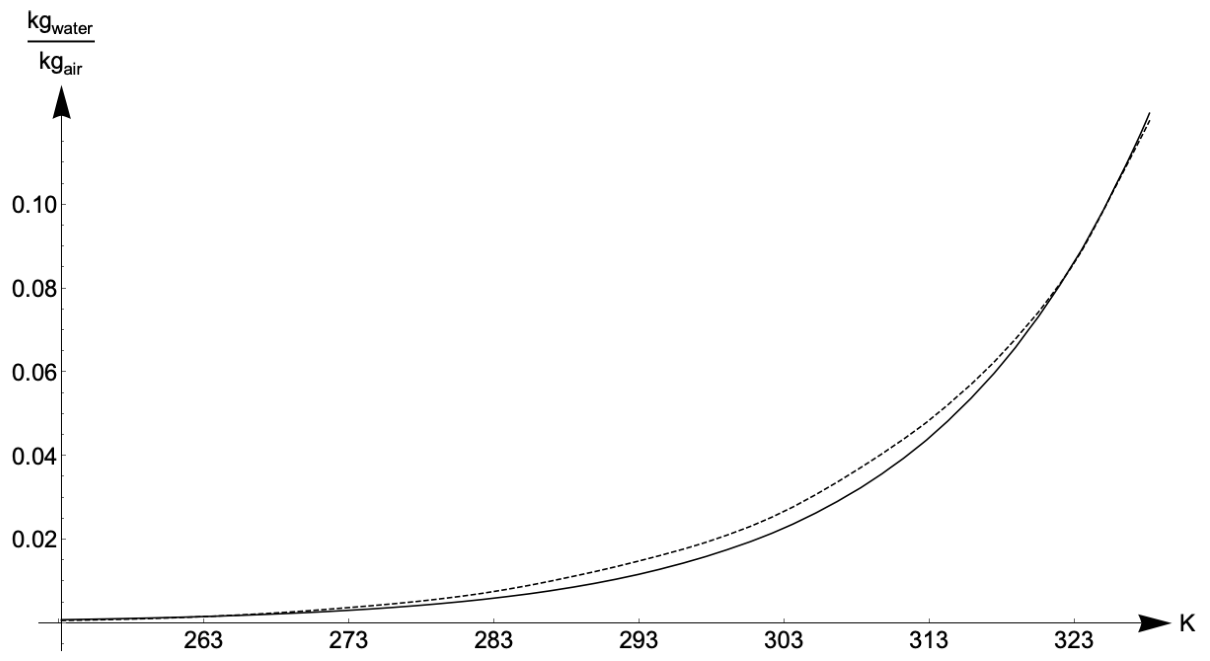
Summarizing, the law that regulates the evolution of humidity in the air is

$$\begin{array}{cc}\hfill {\displaystyle \frac{dU}{dt}}\left(t\right)& =p{\mu }_1(U_s\left(T_0\left(t\right)\right)-U\left(t\right))+q{\mu }_2(U_s\left(T_0\left(t\right)\right)-U\left(t\right))-\nu U\hfill \\ & =(p{\mu }_1+q{\mu }_2)(U_s\left(T_0\left(t\right)\right)-U)-\nu U,\hfill \end{array}$$

(13)

where

$$U_s\left(T\right)=e^{0.0666T-23.96}$$

(14)

is the humidity of saturation, a function of the air temperature T whose values are the maximal amount of kg of water vapour that a kg of dry air can contain. This function has been obtained fitting well known values, its graph is represented in Figure 3.

3.6. Latent Heat of Evaporation and Condensation

As we have seen in last section, humidity plays a crucial role in the thermodynamics of the system under investigation. In fact, given a certain temperature and atmospheric composition, evaporation and condensation of water take place, depending on the difference between the absolute humidity and the saturation humidity. As we know, for each phase transition there is a latent heat, that is heat used for phase transition. During the process of evaporation part of the solar energy is used to change from liquid to vapour phase. That energy is not used to increase the temperature of the thermodynamic body. Therefore, if the mass of water undergoing evaporation per unit time and area is given by ${\rho }_0{\ell }_{0}dU/dt>0$, the related latent heat of evaporation is given by the formula

$${\displaystyle \frac{d{Q}_1^{LE}}{dt}}=-p\lambda {\rho }_0{\ell }_0{\frac{dU}{dt}}^{+},{\displaystyle \frac{d{Q}_2^{LE}}{dt}}=-q\lambda {\rho }_0{\ell }_0{\frac{dU}{dt}}^{+},$$

(15)

where $\lambda$ is the specific latent heat for evaporation of water [22] and the superscript + indicates the “positive part”. If $dU/dt<0$, the opposite process, called condensation, takes place. During this process, heat is released to the environment, with the same law as that for evaporation. In our system, the latent heat of condensation is released directly to the atmosphere, with the law

$${\displaystyle \frac{d{Q}_0^{LC}}{dt}}=\lambda {\rho }_0{\ell }_0{\frac{dU}{dt}}^{-},$$

(16)

where the superscript “−” indicates the “negative part” (which is non-negative). Averaging for the year, it is known that heat exchanged through these processes amounts to about 25% of the solar irradiance [23]. To compare the magnitude of this process, heat transfer through convection amounts to about $5\%$ of the solar irradiance, and the energy absorbed directly by the atmosphere is between $18\%$ and $25\%$ of solar irradiance.

3.7. Thermal Inertia

Under the effect of heat transfers, the rate at which the temperature of a thermodynamic body change depends on its thermal capacity. In our case

$$\frac{d{Q}_0}{dt}=C_0\left(U\right)\frac{d{T}_0}{dt},\frac{d{Q}_1}{dt}=p{C}_1\frac{d{T}_1}{dt},\frac{d{Q}_2}{dt}=q{C}_2\frac{d{T}_2}{dt}.$$

(17)

The parameters $C_i$ are the thermal capacities per unit surface ($\mathrm{J}{\mathrm{K}}^{-1}{\mathrm{m}}^{-2}$). For a body i with density ${\rho }_i$ ($\mathrm{kg}/{\mathrm{m}}^3$), specific heat capacity $c_i$ ($\mathrm{J}\mathrm{K}\mathrm{kg}$), and depth ${\ell }_i$, the thermal capacity per unit surface is $C_i={\rho }_i{c}_i{\ell }_i$. We will assume the thermal capacities constant for all thermodynamic bodies except for the air. This is justified by the fact that the thermal capacity of the air depends on its content of water vapour. Recalling that U is the absolute humidity of the air, measured in kg of water per kg of air, we will assume that the heat capacity of the air is

$$C_0\left(U\right)=c_0^d{\rho }_0^d{\ell }_0+c_0^v{\rho }_0^d{\ell }_{0}U=C_0^d+C_0^{v}U,$$

where $c_0^d$ is the specific heat capacity of dry air, and $c_0^v$ is the specific heat capacity of water vapour, ${\rho }_0^d$ is the density of dry air, and ${\ell }_0$ is the effective depth of the layer of air. The new independent variable U here introduced will in turn depend, via a differential equation, from the temperature of the air. The specific heat of dry air is $711.28\mathrm{J}\mathrm{kg}\mathrm{K}$, the specific heat of water vapour is $2050.16\mathrm{J}\mathrm{kg}\mathrm{K}$. In our model we consider a layer of lower atmosphere ${\ell }_0=400\mathrm{m}$.

Following [13,16], we choose ${\ell }_1\in [0.3,0.5]\mathrm{m}$ for soil, ${\ell }_2\in [40,60]\mathrm{m}$ for oceans. The thermal characteristics of land and water differ from region to region. For this reason in different cases we use different heat capacities. For details on such values see [14,24,25,26]. Using the arguments above one obtains the values shown in

Table 8. Heat capacities.

Parameter	Value		Description
$C_0^d$	$3.5\times {10}^5$	$\mathrm{J}{\mathrm{K}}^{-1}{\mathrm{m}}^{-2}$	dry air thermal capacity
$C_0^v$	$1\times {10}^6$	$\mathrm{J}{\mathrm{K}}^{-1}{\mathrm{m}}^{-2}$	water vapor thermal capacity
$C_1^{soil}$	$1.0\times {10}^6$	$\mathrm{J}{\mathrm{K}}^{-1}{\mathrm{m}}^{-2}$	soil thermal capacity
$C_1^{ice}$	$1.0\times {10}^6$	$\mathrm{J}{\mathrm{K}}^{-1}{\mathrm{m}}^{-2}$	ice thermal capacity
$C_1^{forest}$	$1.7\times {10}^6$	$\mathrm{J}{\mathrm{K}}^{-1}{\mathrm{m}}^{-2}$	forest thermal capacity
$C_1^{sand}$	$3.2\times {10}^6$	$\mathrm{J}{\mathrm{K}}^{-1}{\mathrm{m}}^{-2}$	sand thermal capacity
$C_2$	$[1.7,2.5]\times {10}^8$	$\mathrm{J}{\mathrm{K}}^{-1}{\mathrm{m}}^{-2}$	ocean thermal capacity

.

3.8. Final System

Summarizing Equations (4), (5), (7)–(11), (13) and (15)–(17), with some minimal algebra, the dynamical system that models the temperature evolution of $\mathcal{R}$ is modelled by the evolution of the 4 independent variables $T_0,T_1,T_2,U$, and the variable $\vartheta$, whose evolution is fixed for planet Earth,

$$\left\{\begin{array}{c}(C_0^d+U{C}_0^v)\frac{d{T}_0}{dt}={\alpha }_0(1+p{\tau }_0{r}_1+q{\tau }_0{r}_2)W+\sigma {\alpha }_0^T(p{\epsilon }_1{T}_1^4+q{\epsilon }_2{T}_2^4)+\hfill \\ -\sigma ({\epsilon }_0^d+{\epsilon }_0^u)T_0^4+p{h}_{01}(T_1-T_0)+q{h}_{02}(T_2-T_0)+\lambda {\rho }_0{\ell }_0{\frac{dU}{dt}}^{-}\hfill \\ C_1\frac{d{T}_1}{dt}={\tau }_0{\alpha }_{1}W+\sigma ({\epsilon }_0^d{T}_0^4-{\epsilon }_1{T}_1^4)-h_{01}(T_1-T_0)+{\eta }_1-\lambda {\rho }_0{\ell }_0{\frac{dU}{dt}}^{+}\hfill \\ C_2\frac{d{T}_2}{dt}={\tau }_0{\alpha }_{2}W+\sigma ({\epsilon }_0^d{T}_0^4-{\epsilon }_2{T}_2^4)-h_{02}(T_2-T_0)+{\eta }_2-\lambda {\rho }_0{\ell }_0{\frac{dU}{dt}}^{+}\hfill \\ \frac{dU}{dt}=(p{\mu }_1+q{\mu }_2)U_s\circ T_0-(p{\mu }_1+q{\mu }_2+\nu )U\hfill \\ \frac{d\vartheta }{dt}={\displaystyle \frac{2\pi }{Y{\sqrt{1-e^2}}^3}}{(1+ecos\vartheta )}^2.\hfill \end{array}\right.$$

(18)

4. Numerical Analysis

In this section we choose regions with various types of climate. For each region we choose the parameters depending on its climatic type, and we run the simulation of the model proposed above. We then compare the plots of the numerical computed temperatures and humidities with those of the real averaged ones. The numerics, the acquisition of real temperatures, and their manipulation have been done using the software Mathematica Wolfram Research Inc. [27]. In particular WeatherData[] allowed us to acquire the dataseries of temperatures and humidity with respect to coordinated universal time (UTC) from weather stations belonging to a variety of different Köppen climates. The real temperatures are averaged over a period of 48 years (from 1973 to 2020) using a sampling step of 60 min whenever possible. The creation of the datasets, the numerical simulation of temperature and humidity, the comparison of the results, can all be produced using the Mathematica notebook provided in the supplementary material.

We consider 5 regions: Hilo–Hawaii, Kufra–Lybia, Catania–Italy, Lincoln–USA, Vostok–Antarctica. Each region belongs to one of the Köppen climate zones [12]: Tropical (A), Arid (B), Temperate (C), Continental (D), and Polar (E), respectively. In the following subsections we choose the local parameters by taking into consideration the type of climate and surface composition and by optimising them in their given ranges. For each simulation we estimate its accurateness by computing a discretized $L_1$-distance,

$$dist(T_{re},T_{sim})=\frac{1}{24\ast 365}\sum _{i=1}^{24\ast 365}\left|T_{re}\left(t_i\right)-T_0\left(t_i\right)\right|,$$

where $T_{re}\left(t_i\right)$ are the average real values of temperature at the $24\ast 365$ times $t_i$ equally distributed during a year made by the meteorological stations (assuming we have 24 measures per day), and $T_0\left(t_i\right)$ are the values of the function $T_0$ solutions of our model at the same times (same for humidity separately). The plot comparison is done superimposing the real mean temperature and humidity with those obtained with our model for each region. In the yearly plots we indicate with dashed lines the solstices and equinoxes; in the daily plots we indicate middays and midnights.

4.1. Tropical Climate: Hilo, Hawaii

Hilo belongs to a region with Tropical, Rainforest Köppen climate (AF type). It is situated at latitude $19.72$ and longitude $-155.05$. Belonging to an Hawaiian island, we choose $p=0.05$. The presence of forest makes it reasonable to choose an higher value for the land’s thermal capacity $C_1=1.7\times {10}^6\mathrm{J}{\mathrm{K}}^{-1}{\mathrm{m}}^{-2}$, while considering ${\ell }_2=50\mathrm{m}$ for oceans gives $C_2=2.1\times {10}^8\mathrm{J}{\mathrm{K}}^{-1}{\mathrm{m}}^{-2}$. We also consider the following values for other location-dependent parameters:

$$\begin{array}{cc}& {\alpha }_0^T=0.8,h_{01}=1\frac{\mathrm{J}}{\mathrm{s}{\mathrm{m}}^2},h_{02}=43\frac{\mathrm{J}}{\mathrm{s}{\mathrm{m}}^2},\hfill \\ & p{\mu }_1+q{\mu }_2=1\times {10}^{-5}{\mathrm{s}}^{-1}{\mathrm{m}}^{-2},\nu =0.3\times {10}^{-5}{\mathrm{s}}^{-1}{\mathrm{m}}^{-2}.\hfill \end{array}$$

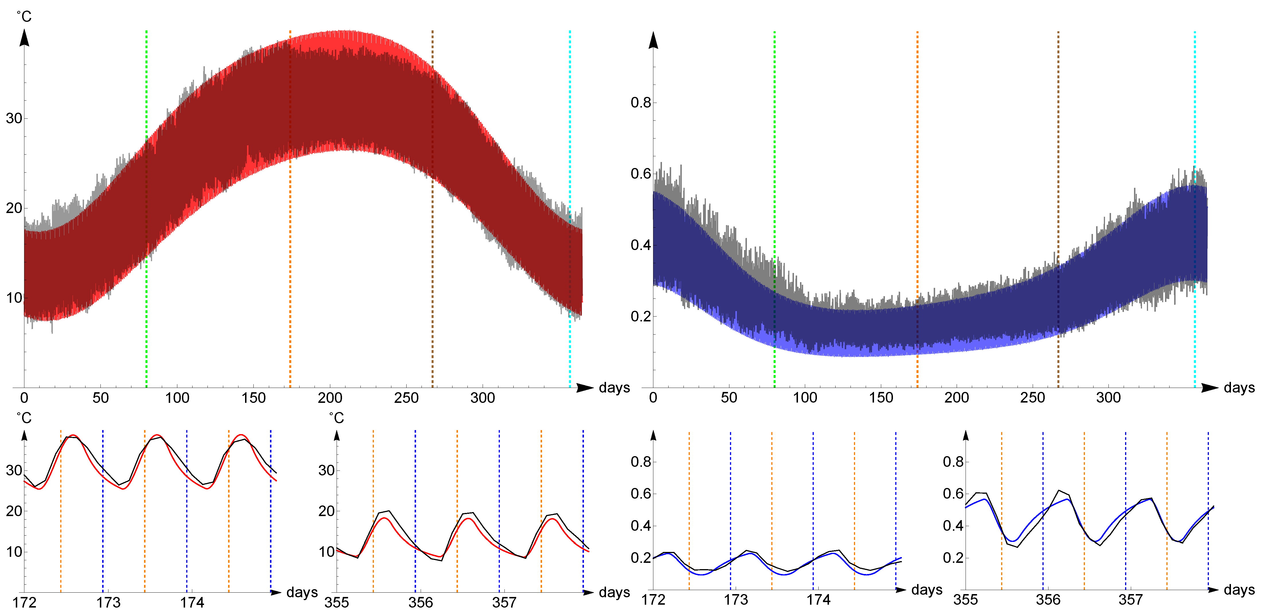
The computed evolution of temperature (red) and humidity (blue) of the air and the real averaged temperatures and humidities (black) from 1973 to 2020 are represented in Figure 4. The $L_1$ distance of the temperatures is $0.60K$, of the relative humidities is $0.036$.

4.2. Arid Climate: Kufra, Libya

Kufra belongs to the eastern part of Sahara with Arid, Hot Desert (BWH type) Köppen climate. It is situated at latitude 24.18 and longitude 23.31. Being in a desert, water has almost no influence and we hence have chosen $p=0.88$. We use the parameters of sand $C_1,r_1,{\alpha }_1,{\epsilon }_1$ in Table 3, Table 4 and Table 8, the optimal parameters for this type of climate are ${\ell }_2=40\mathrm{m}$ and

$$\begin{array}{cc}& {\alpha }_0^T=0.89,h_{01}=9.5\frac{\mathrm{J}}{\mathrm{s}{\mathrm{m}}^2},h_{02}=23\frac{\mathrm{J}}{\mathrm{s}{\mathrm{m}}^2},\hfill \\ & p{\mu }_1+q{\mu }_2=3.4\times {10}^{-8}{\mathrm{s}}^{-1}{\mathrm{m}}^{-2},\nu =1.3\times {10}^{-7}{\mathrm{s}}^{-1}{\mathrm{m}}^{-2}.\hfill \end{array}$$

The computed evolution of temperature (red) and humidity (blue) of the air and the real averaged temperatures and humidities (black) from 1973 to 2020 are represented in Figure 5. In this case the sampling rate is every 3 h. The $L_1$ distance of the temperatures is $1.16\mathrm{K}$, of the relative humidities is $0.026$.

Being on a desert, in this case the chosen evaporation and rainfall parameters are very low. This is necessary to reproduce the large annual variability of humidity observed in the data.

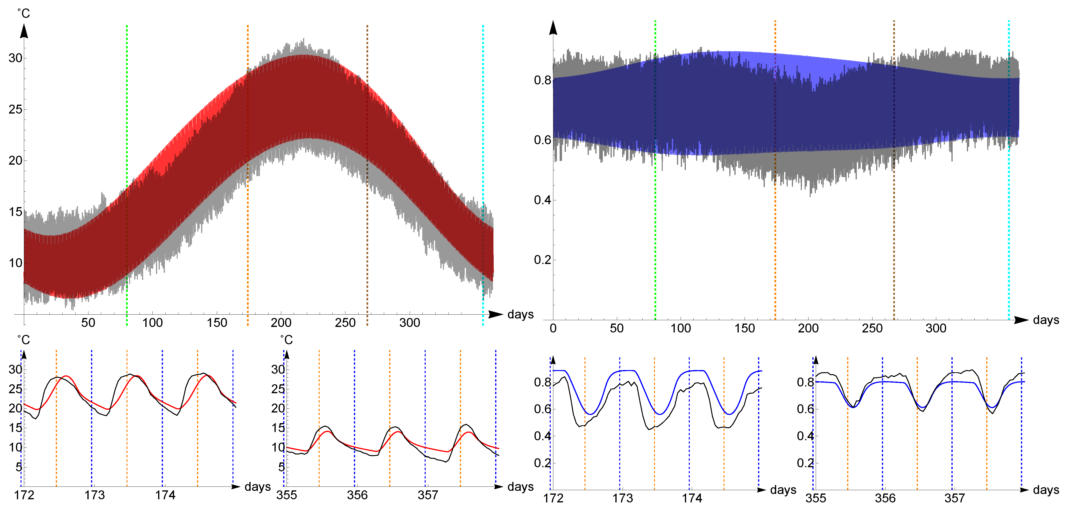
4.3. Temperate Climate: Catania, Italy

Catania is one of the cities on the Mediterranean Sea with Temperate, Hot-summer, Mediterranean Köppen climate (CSA type). It is situated at latitude 37.47 and longitude $15.05$. Given its location, we choose $p=0.6$. Considering that the top layer of Mediterranean sea mix to a depth of up to ${\ell }_2=40\mathrm{m}$, we consider the optimal parameters

$$\begin{array}{cc}& {\alpha }_0^T=0.86,h_{01}=12\frac{\mathrm{J}}{\mathrm{s}{\mathrm{m}}^2},h_{02}=28.5\frac{\mathrm{J}}{\mathrm{s}{\mathrm{m}}^2},\hfill \\ & p{\mu }_1+q{\mu }_2=2.8\times {10}^{-5}{\mathrm{s}}^{-1}{\mathrm{m}}^{-2},\nu =1\times {10}^{-5}{\mathrm{s}}^{-1}{\mathrm{m}}^{-2}.\hfill \end{array}$$

In Figure 6 the computed evolution of temperature (red) and humidity (blue) of the air and the real averaged temperatures and humidities (black) from 1973 to 2020 are represented. The $L_1$ distance of the temperatures is $1.42\mathrm{K}$, of the relative humidities is $0.052$.

4.4. Continental Climate: Lincoln, USA

Lincoln belongs to the central USA, a region with Continental, Hot-summer, Humid Köppen climate (DFA type). It is situated at latitude $40.85$ and longitude $-96.75$. For its location, we choose $p=0.79$, ${\ell }_2=40\mathrm{m}$. We adopt the optimal parameters

$$\begin{array}{cc}& {\alpha }_0^T=0.84,h_{01}=8.5\frac{\mathrm{J}}{\mathrm{s}{\mathrm{m}}^2},h_{02}=22\frac{\mathrm{J}}{\mathrm{s}{\mathrm{m}}^2},\hfill \\ & p{\mu }_1+q{\mu }_2=2\times {10}^{-5}{\mathrm{s}}^{-1}{\mathrm{m}}^{-2},\nu =9.7\times {10}^{-6}{\mathrm{s}}^{-1}{\mathrm{m}}^{-2}.\hfill \end{array}$$

The computed evolution of temperature (red) and humidity (blue) of the air and the real averaged temperatures and humidities (black) from 1973 to 2020 are represented in Figure 7. The $L_1$ distance of the temperatures is $1.38\mathrm{K}$, of the relative humidities is $0.039$.

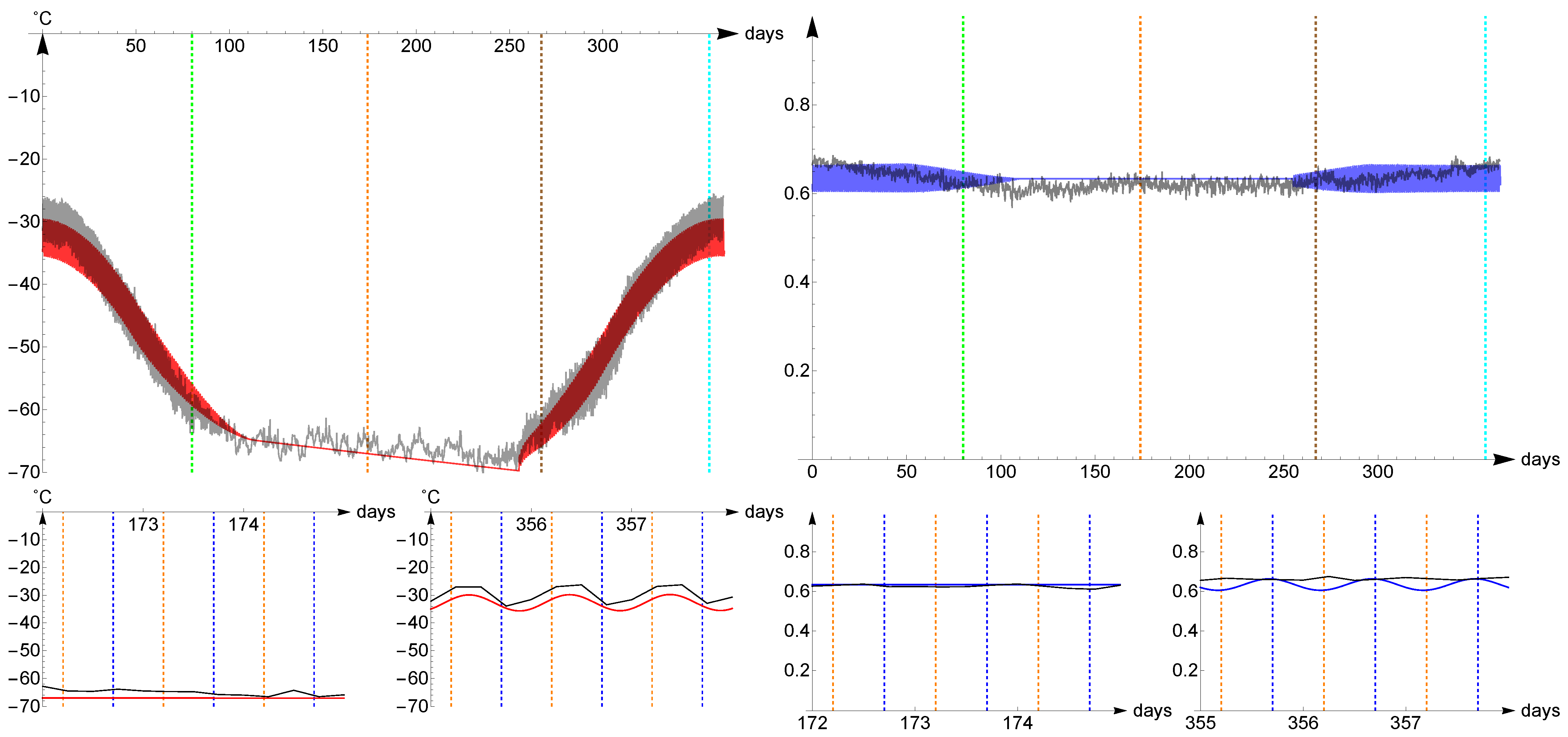
4.5. Polar Climate: Vostok, Antarctica

Vostok is a weather station close to a lake in Antartica, it is located almost at the South Pole and it has Polar, Ice cap Köppen climate (EF type). This region is situated at latitude $-78.45$ and longitude $106.87$ and is always covered with ice and snow, living in eternal winter. The thermal inertia of the ice cap is very high and so, even if located on land, we have chosen $p=0.425$ and the optimal parameters are

$$\begin{array}{cc}& {\alpha }_0^T=0.75,h_{01}=16\frac{\mathrm{J}}{\mathrm{s}{\mathrm{m}}^2},h_{02}=6\frac{\mathrm{J}}{\mathrm{s}{\mathrm{m}}^2},\hfill \\ & p{\mu }_1+q{\mu }_2=1.9\times {10}^{-4}{\mathrm{s}}^{-1}{\mathrm{m}}^{-2},\nu =1.1\times {10}^{-4}{\mathrm{s}}^{-1}{\mathrm{m}}^{-2}.\hfill \end{array}$$

All other parameters are in the Tables, and we have used the coefficients for ice over land and over water.

The computed evolution of temperature (red) and humidity (blue) of the air and the real averaged temperatures and humidity (black) from 1973 to 2020 are represented in Figure 8. The sampling rate in this case is made every 6 h. The $L_1$ distance of the temperatures is $1.76\mathrm{K}$, of the relative humidities is $0.021$.

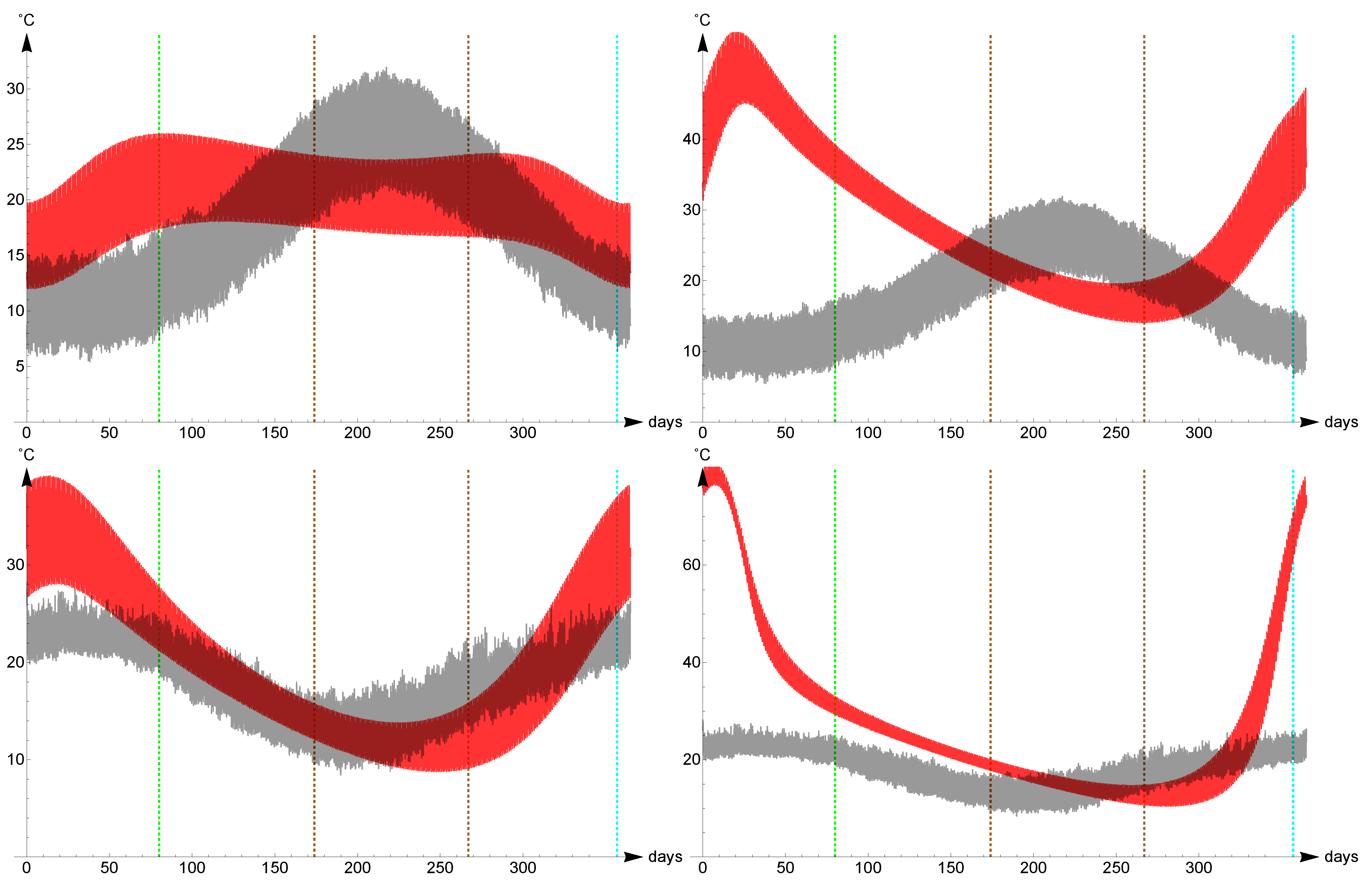
4.6. More Eccentric Cases

The long-time stability of the orbital parameters of Earth is still a debated problem [28]. In our model the orbital parameters can be easily changed to model the temperatures in an Earth-like planet. The small eccentricity of the orbits in the solar system are well known to be non-generic [29]. In the following plots we investigate the temperatures that Catania would have if the eccentricity of Earth was $e=0.2$ or $e=0.5$, and we compare the same effect on Sydney, a city in the southern hemisphere. We recall that, because of Earth’s orientation of the rotation axis, during the summer of the northern hemisphere the Earth is at the aphelion, while during the summer of the southern hemisphere the Earth is at the perihelion. It follows that the effect of a change in eccentricity is mild in Catania (see Figure 9 top) and severe in Sydney (see Figure 9 bottom). Let us note however that the precession of the equinoxes would switch the situation every half Platonic year (12,886 years).

Similar speculations could be applied to exoplanets, whose habitability has been highly investigated in the last decade. Our simple model could help validate or broaden information on astronomical parameters and composition of the surface of the planet [30,31].

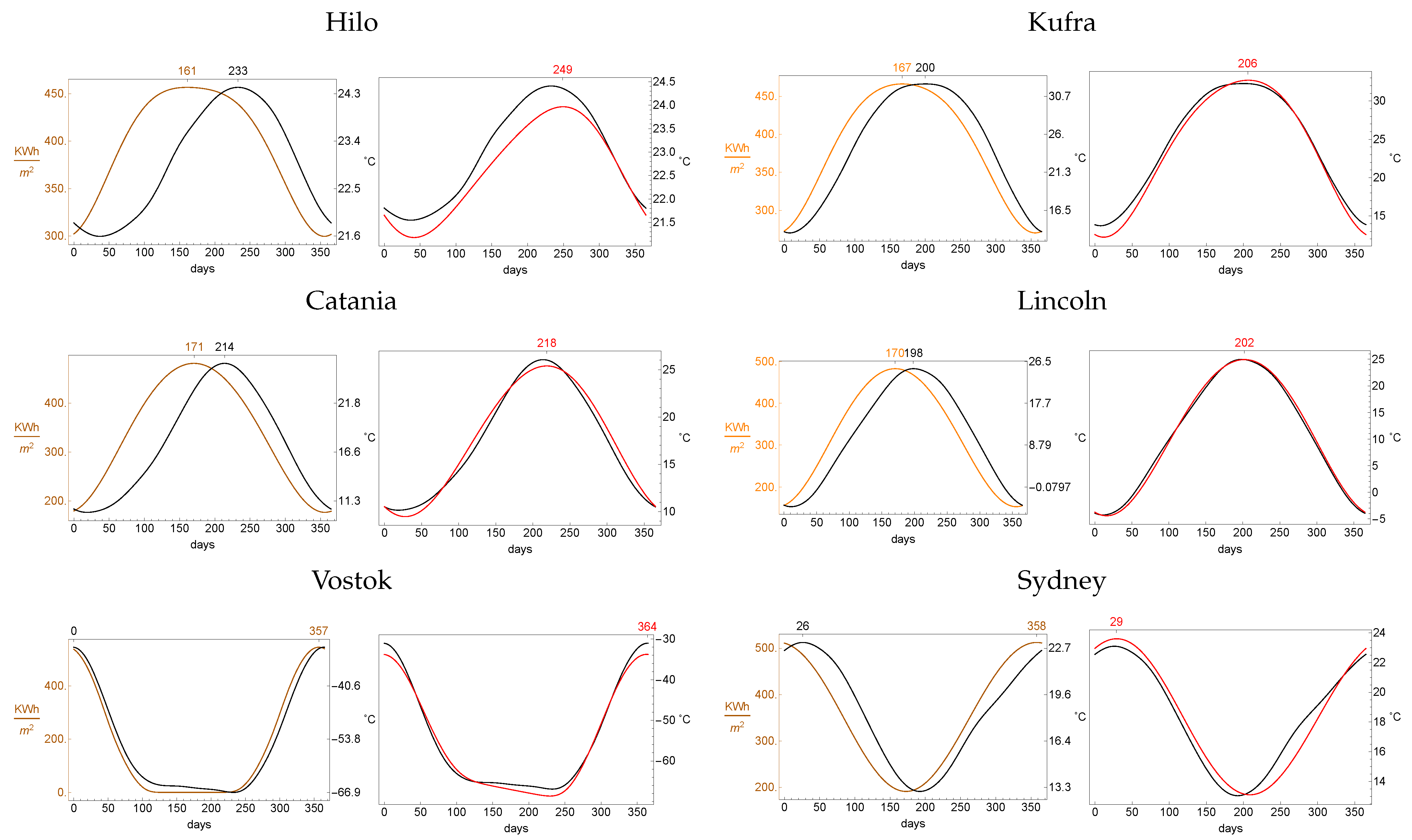
5. Analysis of the Lags

In Figure 10 we expose the phenomenon of the lag of seasons in the six locations examined in the previous section. In Orange we plot the energy that a square meter of higher atmosphere receives from the sun each day of the year. In black we plot the recorded average temperature of that day, in red the simulated average temperature. The days of highest average temperature and highest solar irradiation are then computed estimating the maximum with the Mathematica function FindArgMax[]. The real lag oscillates between the 23 days of Lincoln and the 72 days of Hilo (the special case of Vostok has a lag of only 8 days). The relative error of our simulated lag with respect to the real one is small.

The lag of noon is a much more delicate issue, mainly because the datasets retrieved do not have a time-step fine enough to allow this type of analysis. For each zone, we have computed the time of highest temperature during each day, and we have averaged that time over the year. We compare the results in

Table 9. Average time of daily maximal solar irradiation, and average times of daily maximal temperature measured and simulated.

City	Max Power of Solar Rad.	Max Temp.	Max Simulated Temp.
Hilo	22 h 21 m UTC	23 h 21 m UTC	0 h 9 m UTC
Kufra	10 h 27 m UTC	14 h 43 m UTC	13 h 46 m UTC
Catania	11 h 00 m UTC	11 h 50 m UTC	14 h 04 m UTC
Lincoln	18 h 27 m UTC	21 h 23 m UTC	22 h 00 m UTC
Sydney	1 h 56 m UTC	3 h 45 m UTC	4 h 55 m UTC

.

The lag is highly sensitive to the depth of the atmospheric layer, and our estimated lag is typically later than the measured one, sometimes much later, and earlier in the case of Kufra, which is not so significant since in that case the temperatures are measured every 3 h. A change in the depth of the atmospheric layer we consider can adjust not only this number, but also noticeably improve the simulations. For example in Lincoln one can obtain a simulated temperature evolution whose $L_1$ distance from the real one is $1.10\mathrm{K}$ and the new average time of maximal simulated temperature takes place at 21 h 12 m. For Catania the same distance and time are $1.07\mathrm{K}$ and 13 h 06 m. A justification of these facts goes beyond the scope of this paper.

6. Conclusions

In this article, starting from basic physical laws, the dynamics of solar systems, and the structure of a given planet, we design a simple model able to reproduce basic features of local climates (based on Köppen climatic zones). Although the proposed model has been developed for a generic planet, our investigation is here restricted to Earth, for which the parameters involved are mostly given by experimental evidence. Once chosen a region on Earth, and fitted some parameters, the model reproduces the evolution of temperatures of land, water, air and its humidity. In doing so it also reproduces climatic phenomena like seasonal lag, diurnal lag, daily asymmetry of temperatures variations.

The simulated temperatures, computed solving the equations, are similar to the real ones. In particular, as the real temperatures, they display lags and asymmetric daily evolution. They could have a better behaviour adding other phenomena to the equations. Despite the fact that humidity creates an asymmetric raise and fall of temperatures, the raise of real temperatures in the morning is often faster than simulated ones.

The model still displays some criticality and it can be improved in many ways. In particular we indicate the following issues:

• the model requires the inclusion of some water also when dealing with desert or ice-caps, because the stabilising effect of water is necessary to avoid too high annual temperature excursions;
• we only consider the lowest part of the atmosphere;
• spatial diffusion has been disregarded;
• the equations that model humidity is not completely satisfactory, it probably should take into account other factors;
• altitude in not considered explicitly;
• absorbance, transmittance and reflectance should be dependent on the solar zenith angle.

The first and second issues could be dealt with by adding other layers, one below the soil and one above the lower atmosphere. This would grant a better annual excursion without compromising the daily one.

The spatial diffusion has been intentionally excluded to keep the model as simple as possible. The introduction of diffusion completely changes the approach, forcing a discretisation of the surface of the planet and the creation of a GCM which requires a detailed description of the planet surface and a large computational effort. In this manuscript we compensate the lack of meridional heat transport by a slight change in the effective absorbance parameters.

The evaporation depends on wind velocity, and probably non-constant wind speed should be taken into account, as well as seasonal variations in the rainfall rate. We have not made a deep investigation on this facts, and we do not propose solutions.

Altitude can very likely be modelled with a change of absorbance, transmittance and reflectance, because at higher altitudes the air pressure is lower. In this manuscript we do not take into consideration pressure variations, but we have a minor discretionality in the choice of the parameters.

Radiation parameters of the atmosphere should change with the solar zenith angle, because of the laws of optics and because the depth of the atmospheric section crossed by the solar rays depends on such angle. Also diffraction could be taken into consideration with small changes. Similar considerations can be made for oceanic and land surfaces.

The investigation is suitable for applications to exoplanets. Some astronomical parameters of exoplanets are known, but the choice of most other parameters is a delicate issue and will be subject of future works. In particular we think that the model could be useful in the investigation of habitable and tidally locked planets.

In conclusion, we reckon that this article convincingly demonstrates the existence of a connection between the three phenomena discussed and the existence of two thermodynamic bodies with different thermal inertia and a varying humidity.