Prediction of Multi-Scalar Standardized Precipitation Index by Using Artificial Intelligence and Regression Models

Abstract

Accurate monitoring and forecasting of drought are crucial. They play a vital role in the optimal functioning of irrigation systems, risk management, drought readiness, and alleviation. In this work, Artificial Intelligence (AI) models, comprising Multi-layer Perceptron Neural Network (MLPNN) and Co-Active Neuro-Fuzzy Inference System (CANFIS), and regression, model including Multiple Linear Regression (MLR), were investigated for multi-scalar Standardized Precipitation Index (SPI) prediction in the Garhwal region of Uttarakhand State, India. The SPI was computed on six different scales, i.e., 1-, 3-, 6-, 9-, 12-, and 24-month, by deploying monthly rainfall information of available years. The significant lags as inputs for the MLPNN, CANFIS, and MLR models were obtained by utilizing Partial Autocorrelation Function (PACF) with a significant level equal to 5% for SPI-1, SPI-3, SPI-6, SPI-9, SPI-12, and SPI-24. The predicted multi-scalar SPI values utilizing the MLPNN, CANFIS, and MLR models were compared with calculated SPI of multi-time scales through different performance evaluation indicators and visual interpretation. The appraisals of results indicated that CANFIS performance was more reliable for drought prediction at Dehradun (3-, 6-, 9-, and 12-month scales), Chamoli and Tehri Garhwal (1-, 3-, 6-, 9-, and 12-month scales), Haridwar and Pauri Garhwal (1-, 3-, 6-, and 9-month scales), Rudraprayag (1-, 3-, and 6-month scales), and Uttarkashi (3-month scale) stations. The MLPNN model was best at Dehradun (1- and 24- month scales), Tehri Garhwal and Chamoli (24-month scale), Haridwar (12- and 24-month scales), Pauri Garhwal (12-month scale), Rudraprayag (9-, 12-, and 24-month), and Uttarkashi (1- and 6-month scales) stations, while the MLR model was found to be optimal at Pauri Garhwal (24-month scale) and Uttarkashi (9-, 12-, and 24-month scales) stations. Furthermore, the modeling approach can foster a straightforward and trustworthy expert intelligent mechanism for projecting multi-scalar SPI and decision making for remedial arrangements to tackle meteorological drought at the stations under study.

1. Introduction

Drought is a crucial ecological issue impacting Earth and humans. Drought refers to water scarcity, severely impacting society’s different segments, such as hydropower, agriculture, industrial, and water supply. The crucial factors for assessing the drought severity include period, location in absolute time, i.e., start and closure time points, areal coverage, and scale or force [1]. Wilhite and Glantz [2] deployed theoretical and operational expressions for describing a drought. The theoretical definition of drought is expressed generally as the shortage of precipitation causing harm to crops and harvest. The theoretical definition is vital for setting up a drought policy. The operational description aids people to determine the commencement, rigorousness, and conclusion period of the drought based on 30-year records by comparing the present situation with the historical average (recommended by the World Meteorological Organization). In general, operational droughts can be utilized for ascertaining drought frequency, rigorousness, and span for a specific return period [3]. Several drought classifications are mentioned in the literature; however, they are usually categorized into three main classes: (1) meteorological drought—a scenario where the shortage of precipitation is over 25% from the normal or average volume over an area for some time; (2) hydrological drought—a scenario where the resources of surface water and groundwater begin to exhaust from a marked level; and (3) agricultural drought—a scenario where the soil moisture and rainfall are insufficient in the growing season to boost vigorous crop growth until maturity.

The right choice of input variables [4,5] is vital for drought estimation. Understanding that a shortage of precipitation impacting streamflow, soil moisture, groundwater level, and reservoir storage led to the Standardized Precipitation Index (SPI) [6]. The SPI was constructed to calculate the precipitation deficit on various time scales and manage the impact of drought on the available water resources. For the computation of SPI long term (>30 years), precipitation data are fitted to a suitable probability distribution and then transformed into a normal distribution. In the last year, research activities were carried out on drought projection by utilizing different stochastic and artificial intelligence (hybrid or simple) models. Mishra and Desai [7] assessed the prospect of the seasonal-autoregressive integrated moving average (SARIMA) for drought projection in the Kansabati River Basin (India) by deploying multi-scalar SPI. According to available literature, all models can be deployed effectively for drought projection over varying lead times in the study area. Morid et al. [8] applied ANN (artificial neural network) for projecting meteorological drought in Tehran, Iran, province by utilizing the SPI, EDI (Effective Drought Index), and SOI (Southern Oscillation Index) as well as NAO (North Atlantic Oscillation) index. The observations indicated that the ANN could be deployed to a great extent for drought projection in the study area. Bacanli et al. [9] deployed FFNN (Feed Forward Neural Networks) and ANFIS (Adaptive Neuro-Fuzzy Inference System) for estimation of meteorological drought based on SPI-1 and SPI-12 in Turkey. Results revealed the superiority of the ANFIS models over the FFNN models. Belayneh and Adamowski [10] made a comparison of the ability of SVR (Support Vector Regression), ANN, and WNN (Wavelet Neural Networks) for projecting meteorological drought based on SPI-3 and SPI-12 in Awash River Basin, Ethiopia. The observations showed that the WNN models outperformed other models. Özger et al. [11] made a comparison of the performances of ANN, Wavelet-Fuzzy Logic (WFL), and Wavelet-ANN (WANN) models for projecting drought in Texas based on PMDI (Palmer Modified Drought Index) and ENSO (El Nino-Southern Oscillation). They noted that the WFL models performed better than other models.

Recently, several applications of Artificial Intelligence (AI)-based models have been observed for meteorological drought estimation on a global level. Deo and Şahin [12] studied ANN’s prospect for meteorological drought projection based on SPEI (standardized precipitation evapotranspiration index) at eight stations in eastern Australia 1915–2005. They noted the better utility of ANN models in projecting the SPEI over the study sites. Nguyen et al. [13] projected short- and long-term droughts by deploying ANFIS based on SPEI and SPI at CRB (Cai River basin), Vietnam. Results showed the ANFIS model’s better viability for predicting long-term SPEI (12-month) and short-term SPI (1- and 3-month) in the study basin. Djerbouai and Souag-Gamane [14] utilized WANN, ANN, SARIMA, and ARIMA models for SPI-3, SPI-6, and SPI-12 prediction Algerois basin, Algeria, and they found that the WANN model outperformed the other models. Deo et al. [15] deployed WELM (Wavelet-Extreme Learning Machine), WANN, WLSSVR (Wavelet-Least Squares Support Vector Regression), LSSVR (Least Squares Support Vector Regression), and ANN models for drought estimation based on EDI in Australia. Outcomes indicated that the WELM models had a better performance than the LSSVR, ANN, WANN, and WLSSVR models. Komasi et al. [16] evaluated the SVM (Support Vector Machine), WSVM (Wavelet-Support Vector Machine), and CS-SVM (Cuckoo Search-Support Vector Machine) for drought estimation based on SPI in Urmia Lake watershed, Iran. The performance of the WSVM model was better compared to the other models. Abbasi et al. [17] studied the meteorological drought in Urmia Lake (Iran) based on multi-scalar SPI and SPEI, and the projection was conducted by utilizing the Gene Expression Programming (GEP) model. The drought took place during 1959–1967 and 1998–2009. The observations indicated that the GEP model’s superiority increased by mounting the scale of SPI and SPEI.

With related context, Memarian et al. [18] applied the CANFIS model to forecast the drought in Birjand (Iran) with the combination of climatic signals, i.e., NINO 1 + 2, NINO 3, Multivariate Enso Index, Tropical Southern Atlantic Index, Atlantic Multi-decadal Oscillation Index, NINO 3.4, and lagged values of SPI. Results highlighted the better feasibility of the CANFIS model in drought forecasting over the study region. Rafiei-Sardooi et al. [19] employed the neuro-fuzzy (NF) and time-series, i.e., ARIMA models, to predict the meteorological drought in the Jiroft plain of Iran using 3- and 12-month SPI. The analysis of results demonstrated that the NF model outperformed the ARIMA model. Malik et al. [20] predicted meteorological drought in the Kumaon region of Uttarakhand State (India) by employing the CANFIS, MLPNN, and MLR models considering SPI-1, SPI-3, SPI-6, SPI-9, SPI-12, and SPI-24. The obtained results were evaluated based on performance measures (i.e., RMSE, NSE, COC, and WI) and revealed that the CANFIS models provided better estimates than other models and different study stations. According to our knowledge, the MLPNN, CANFIS, and MLR models’ efficacy for meteorological drought projection using the Standardized Precipitation Index (SPI) had not yet been investigated in the Garhwal region of Uttarakhand State, India. In this paper, the analysis was carried out by utilizing monthly rainfall data at Chamoli, Dehradun, Haridwar, Pauri Garhwal, Rudraprayag, Tehri Garhwal, and Uttarkashi stations with the three objectives: (1) to calculate the SPI at various time scales, 1-, 3-, 6-, 9-, 12-, and 24-month, by utilizing available rainfall information; (2) to formulate the MLPNN, CANFIS, and MLR models for meteorological drought projection based on nominated input by utilizing the PACF analysis of multi-scalar SPI; and (3) to standardize and corroborate the AI and regression models for prediction of multi-scalar SPI values employing visual and statistical indicators.

2. Materials and Methods

2.1. Study Area and Data Assembly

This study was executed in the Garhwal region of Uttarakhand State (India), situated in the central Himalayan zone, spanning 32,499 km² (Figure 1) among 77°34′ E to 81°03′ E longitudes and 28°43′ N to 31°28′ N latitudes by varying altitudes of 276 m to 5046 m above mean sea level. It borders with Uttar Pradesh in the South, Himachal Pradesh in the northwest, and China and Nepal in the northeast and southeast. Uttarakhand has 13 districts divided into two administrative divisions: (1) Garhwal, which comprises seven districts (Chamoli, Dehradun, Haridwar, Pauri Garhwal, Rudraprayag, Tehri Garhwal, and Uttarkashi) and (2) Kumaon, which comprises six districts (Almora, Bageshwar, Champawat, Nainital, Pithoragarh, and Udham Singh Nagar). The state boasts of a temperate climate, except the plains where it is tropical. The temperature varies from sub-zero to 43 °C. The yearly rainfall falls in 260 mm and 3955 mm, where 60% to 85% occurs during the monsoon season (June to September).

For estimating meteorological drought, seven rain gauge stations were set up, as shown in Figure 1. The information regarding the longitude, latitude, altitude, and data availability are presented in

Table 1. Details of study stations and rainfall data availability.

Meteorological Station	Latitude (N)	Longitude (E)	Altitude (m)	Rainfall Data (Year)
Chamoli	30°46′30″	79°37′41″	5046	1901–2015
Dehradun	30°27′32″	77°53′28″	728	1901–2015
Haridwar	29°55′26″	78°03′04″	276	1901–2015
Pauri Garhwal	29°50′28″	78°43′44″	1134	1901–2015
Rudraprayag	30°36′07″	79°05′53″	2117	1901–2015
Tehri Garhwal	30°26′53″	78°32′42″	1996	1955–2015
Uttarkashi	31°00′47″	78°24′29″	3366	1951–2015

. The data used in this study included monthly rainfall records that were gathered over seven stations from the India Meteorological Department (IMD), Pune.

2.2. Standardized Precipitation Index (SPI)

McKee et al. [6] formulated the SPI to describe, monitor, and examine droughts on various time scales at Colorado State University. A detailed depiction of SPI was presented by Guttman [21] and Hayes et al. [22]. The calculation of SPI for a particular time scale at any location entails long-term (≥30 years) information on monthly precipitation. In general, the SPI is computed by exploiting statistical probability distribution over the aggregated rainfall of different time scales of attention. This activity was carried out individually for every month and location in space. The SPI is calculated by transforming every probability distribution into the standardized normal distribution (Z-distribution). Many research works have been carried out on rainfall distribution by utilizing the different probability distributions [23,24].

In this research, two-parameter gamma distribution [24,25,26] was utilized for the computation process of SPI by using Equation (1) [27,28]:

$$Z=\left\{\begin{array}{cc}SPI = -\left(t-\frac{c_0 + c_{1}t + c_2{t}^2}{1 + d_{1}t + d_2{t}^2 + d_3{t}^3}\right)& \mathrm{for}, 0<H\left(x\right)\le 0.5\hfill \\ SPI = +\left(t-\frac{c_0 + c_{1}t + c_2{t}^2}{1 + d_{1}t + d_2{t}^2 + d_3{t}^3}\right)& \mathrm{for}, 0.5<H\left(x\right)<1.0\hfill \end{array}\right.$$

(1)

in which $c_0, c_1, c_2, d_1, d_2, d_3, \mathrm{and} t$ are constants, and defined as: $c_0=2.515517$, $c_1=0.802853$, $c_2=0.010328$, $d_1=1.432788$, $d_2=0.189269$, and $d_3=0.001308$. $H\left(x\right)$ is the commutative probability, $t=\sqrt{\ln \left[\frac{1}{{\left(H\left(x\right)\right)}^2}\right]}$ for $0<H\left(x\right)\le 0.5$, and $t=\sqrt{\ln \left[\frac{1}{{\left(1-H\left(x\right)\right)}^2}\right]}$ for $0.5<H\left(x\right)<1.0$ [6].

2.3. Co-Active Neuro-Fuzzy Inference System (CANFIS)

To solve the nonlinear optimization problems, Jang et al. [29] projected the idea of the CANFIS technique. In the present time, the CANFIS model effectiveness has been found in numerous fields of sciences [20,30,31,32,33,34]. The basic structure of CANFIS involved integrating ANN and FIS (fuzzy-inference system) in one border. Figure 2 demonstrates the typical structure of the CANFIS model composed of these five layers (i.e., Layer-1: fuzzification, Layer-2: rule, Layer-3: normalization, Layer-4: defuzzification, and Layer-5: fuzzy association). Each input is passed and treated through these layers. By considering two inputs ($x$ and $y$) under the rule of Takagi–Sugeno–Kang (TSK) fuzzy system with IF-THEN rule, we can describe the CANFIS models [35,36]:

$$\mathrm{Rule} 1:IF x is A_1 \mathrm{and} y is B_1 THEN C_1=p_{1}x+q_{1}y+r_1$$

(2)

$$\mathrm{Rule} 2:IF x is A_2 \mathrm{and} y is B_2 THEN C_2=p_{2}x+q_{2}y+r_1$$

(3)

Here, $A_1$, $A_2$, and $B_1$, $B_1$ are the fuzzy sets with $C_1$ and $C_1$ for the inputs $x$ and $y$. $p_1$, $q_1$, $r_1$ and $p_2$, $q_2$, $r_2$ are parameters of the consequent part (Figure 2). The functioning of every layer is defined as [37,38]:

$$Layer-1 \left(fuzzification\right) ={\mu }_{A_i}\left(x\right) \mathrm{and} {\mu }_{B_i}\left(y\right) \mathrm{for} i = 1, 2$$

(4)

$$Layer-2 \left(rule\right) =w_i= {\mu }_{A_i}\left(x\right)\times {\mu }_{B_i}\left(y\right) \mathrm{for} i = 1, 2$$

(5)

$$Layer-3 \left(normalization\right) =\overline{w_i}=\frac{w_i}{{\Sigma }_i{w}_i} i = 1, 2$$

(6)

$$Layer-4 \left(defuzzification\right) =\overline{w_i}{C}_i=\overline{w_i}\left(p_{i}x+q_{i}y+r_i\right) i = 1, 2$$

(7)

$$Layer-5 \left(fuzzy association\right) =\overline{w_i}{C}_i={\displaystyle \sum }_i\overline{w_i}{C}_i=\frac{{\Sigma }_i{w}_i{C}_i}{{\Sigma }_i{w}_i}$$

(8)

In Equation (4), $A_i$ and $B_i$ are the linguistic labels and ${\mu }_{A_i}$ and ${\mu }_{B_i}$ represent the membership functions (MFs) for linguistic labels. In Equation (5), $w_i$ is the weight (or firing strength) associated with inputs ($x$ and $y$). In Equation (6), $\overline{w_i}$ is the normalized firing strength. In this study, through supervised learning, the CANFIS network was designed. For input data classification, the Gaussian (Gauss) MFs were applied along with the TSK (Takagi–Sugeno–Kang) fuzzy model and hyperbolic tangent activation function (for data normalization), and DBD (delta bar delta) algorithm was found to be more potent for multi-scalar SPI prediction at seven study locations.

Figure 2. The architecture of the co-active neuro-fuzzy inference system (CANFIS) model.

Figure 2. The architecture of the co-active neuro-fuzzy inference system (CANFIS) model.

2.4. Multi-Layer Perceptron Neural Network (MLPNN)

MLPNN was first proposed by Haykin [39]. It involves layers of parallel processing elements, known as neurons. Every layer is wholly linked to the next layer through inter-links of weights (W) or strengths. A typical structure of MLPNN models is composed of three layers, Layer-1: input (i), Layer-2: hidden (j), and Layer-3: output (k) with inter-linked weights (W_ij and W_jk) between these layers, as illustrated in Figure 3. We specified the number of hidden layers and neurons by the number of predictands and predictors [40].

In this research, the 2n + 1 (n represents the inputs) concept was exploited to decide the optimal number of neurons in the hidden layer [7,10]. The designed architecture of MLPNN was then applied to forecast the meteorological drought condition at various locations depending on the SPI values used as input at different lags.

2.5. Multiple Linear Regression (MLR)

The degree of association among target parameter (dependent) and two or many independent parameters was determined using MLR and written as [30,33]:

$$Z ={\beta }_0+ {\beta }_1{X}_1+ {\beta }_2{X}_2+, \dots , + {\beta }_k{X}_n$$

(9)

where $Z$ represents the dependent (target) parameter, ${\beta }_0, {\beta }_1,{\beta }_2,\dots {\beta }_k$ are the regression coefficient of the MLR equation, and $X_1, X_2,\dots X_n$ are the independent parameters. Subscript $n$ denotes the number of independent parameters corresponding to $k$ regression coefficient.

2.6. Input Selection and Model Development

Choosing proper inputs is a tedious task, particularly in nonlinear hydrological processes. The SPI-1, -3, -6, -9, -12, and -24 were calculated using long-term monthly rainfall information in this study. The ACF and PACF (autocorrelation function and partial-ACF) were applied for choosing the crucial inputs (lags). Both ACF and PACF were computed by utilizing the expressions below [41,42]:

$$AC{F}_k=\frac{{\sum }_{t=1}^{N-k}\left(Y_t-\overline{Y}\right) \left(Y_{t+k}-\overline{Y}\right)}{{\sum }_{t=1}^N\left(Y_t-\overline{Y}\right) }$$

(10)

$$PAC{F}_{k,k}=\frac{ACF-{\sum }_{j=1}^{k-1}PAC{F}_{k-1,j} AC{F}_{k-1}}{1-{\sum }_{j=1}^{k-1}PAC{F}_{k-1,j} AC{F}_{k-1} }$$

(11)

in which k defines lag through $Y_t$ data series, $\overline{Y}$ designates the average of the whole data series, and N states the data points. Afterward, at a 5% confidence level, the computed values of PACF were tested, portraying upper and lower critical limits (UCL and LCL) by using Equation (12) [43]:

$${\mathrm{CL}}_{\mathrm{upper}/\mathrm{lower}}=\pm \frac{1.96}{\sqrt{N}}.$$

(12)

2.7. Performance Indicators

The performances of AI and regression were assessed with the Nash­–Sutcliffe Efficiency (NSE) [44], Root Mean Squared Error (RMSE) [45], Willmott Index (WI) [46], Coefficient of Correlation (COC) [45], and visual interpretation was by scatter plot and Taylor diagram [47]. These indices are outlined as:

$$RMSE=\sqrt{\frac{1}{N} {\displaystyle \sum }_{i=1}^N{(SP{I}_{obs, i }- SP{I}_{pre,i})}^2} ( 0 < RMSE < \infty )$$

(13)

$$NSE=1-\left[\frac{{\sum }_{i=1}^N{(SP{I}_{obs,i }- SP{I}_{pre,i})}^2}{{\sum }_{i=1}^N{(SP{I}_{obs,i }- \overline{SP{I}_{obs }})}^2}\right] (-\infty < NSE < 1)$$

(14)

$$COC=\frac{{\sum }_{i=1}^N\left(SP{I}_{obs,i }- \overline{SP{I}_{obs }}\right) \left(SP{I}_{pre,i} - \overline{SP{I}_{pre}}\right) }{\sqrt{{\sum }_{i=1}^N{(SP{I}_{obs,i }- \overline{SP{I}_{obs }})}^2 {\sum }_{i=1}^N{(SP{I}_{pre,i} - \overline{SP{I}_{pre}})}^2 } } (-1 < COC < 1)$$

(15)

$$WI=1-\left[\frac{{\sum }_{i=1}^N{(SP{I}_{pre,i} - SP{I}_{obs, i})}^2}{{\sum }_{i=1}^N{(\left|SP{I}_{pre,i} - \overline{SP{I}_{obs }}\right|+\left|SP{I}_{obs,i }- \overline{SP{I}_{obs }}\right|)}^2}\right] (0 < WI \le 1)$$

(16)

where $SP{I}_{obs }$ and $SP{I}_{pre}$ = observed (computed) and predicted multi-scalar SPI for the ith dataset, N = number of observations, $\overline{SP{I}_{obs }}$ and $\overline{SP{I}_{pre }}$ = mean of observed and predicted multi-scalar SPI. $\left|SP{I}_{pre,i} - \overline{SP{I}_{obs }}\right|$ = absolute difference among predicted and observed mean and $\left|SP{I}_{obs,i }- \overline{SP{I}_{obs }}\right|$ = absolute difference among the observed and their mean.

3. Results

3.1. Significant Lags’ Nomination by Using PACF Analysis

Table 2. The partial autocorrelation function (PACF) analysis of multi-scalar standardized precipitation index (SPI) at study stations.

Station	Index	Lag
		1	2	3	4	5	6	7	8	9	10	11	12
Chamoli	SPI-1	0.213 *	0.048	0.021	0.031	0.043	0.045	0.041	0.038	0.063 *	0.081 *	0.074 *	0.135 *
	SPI-3	0.725 *	−0.180 *	−0.150 *	0.236 *	0.000	−0.041	0.146 *	0.058 *	0.040	0.129 *	0.055 *	0.050
	SPI-6	0.881 *	−0.172 *	−0.071 *	−0.042	−0.018	−0.024	0.416 *	−0.002	0.036	−0.016	−0.073 *	−0.072 *
	SPI-9	0.934 *	−0.112 *	−0.025	0.015	−0.038	−0.015	0.011	−0.055 *	−0.031	0.390 *	−0.073 *	−0.062 *
	SPI-12	0.963 *	−0.150 *	−0.001	0.016	−0.048	−0.054 *	−0.037	−0.020	−0.038	−0.083 *	−0.075 *	0.011
	SPI-24	0.949 *	0.342 *	0.149 *	0.025	−0.027	−0.060 *	0.040	0.020	−0.003	−0.047	−0.110 *	−0.068 *
	UCL/LCL	±0.053	±0.053	±0.053	±0.053	±0.053	±0.053	±0.053	±0.053	±0.053	±0.053	±0.053	±0.053
Dehradun	SPI-1	0.134 *	0.019	−0.053	−0.059 *	0.033	−0.031	0.001	−0.005	−0.026	0.031	0.078 *	0.056 *
	SPI-3	0.659 *	−0.176 *	−0.209 *	0.167 *	0.001	−0.095 *	0.072 *	0.017	0.032	0.047	0.047	0.020
	SPI-6	0.818 *	−0.149 *	−0.059 *	−0.009	−0.044	−0.111 *	0.250 *	0.014	0.037	0.034	0.002	−0.089 *
	SPI-9	0.875 *	−0.054 *	0.072 *	0.018	−0.002	−0.046	−0.044	−0.099 *	−0.135 *	0.279 *	0.044	0.008
	SPI-12	0.951 *	−0.169 *	−0.057 *	−0.001	−0.020	−0.050	−0.030	−0.048	−0.047	−0.083 *	−0.049	−0.022
	SPI-24	0.932 *	0.289 *	0.084 *	0.018	0.003	0.028	0.146 *	0.074 *	−0.008	−0.085 *	−0.093 *	−0.061 *
	UCL/LCL	±0.053	±0.053	±0.053	±0.053	±0.053	±0.053	±0.053	±0.053	±0.053	±0.053	±0.053	±0.053
Haridwar	SPI-1	0.101 *	0.008	−0.037	−0.081 *	0.029	−0.015	−0.020	−0.003	−0.044	0.032	0.010	0.039
	SPI-3	0.639 *	−0.141 *	−0.246 *	0.165 *	0.000	−0.101 *	0.078 *	−0.013	−0.022	0.001	−0.008	0.005
	SPI-6	0.796 *	−0.109 *	−0.079 *	−0.032	−0.042	−0.192 *	0.237 *	−0.021	−0.022	−0.014	−0.056 *	−0.074 *
	SPI-9	0.857 *	0.030	−0.035	−0.060 *	−0.047	−0.072 *	−0.068 *	−0.116 *	−0.208 *	0.288 *	0.012	0.026
	SPI-12	0.924 *	−0.143 *	−0.079 *	−0.033	−0.029	−0.065 *	−0.064 *	−0.054 *	−0.100 *	−0.110 *	−0.100 *	−0.044
	SPI-24	0.870 *	0.287 *	0.073 *	−0.007	−0.018	0.068 *	0.112 *	0.052	−0.033	−0.103 *	−0.103 *	−0.058 *
	UCL/LCL	±0.053	±0.053	±0.053	±0.053	±0.053	±0.053	±0.053	±0.053	±0.053	±0.053	±0.053	±0.053
Pauri Garhwal	SPI-1	0.210 *	0.033	0.013	−0.041	0.058 *	0.002	0.005	0.016	−0.019	0.057 *	0.073 *	0.084 *
	SPI-3	0.696 *	−0.145 *	−0.140 *	0.181 *	0.017	−0.047	0.058 *	0.005	0.051	0.075 *	0.051	0.047
	SPI-6	0.857 *	−0.103 *	−0.042	−0.043	−0.001	−0.109 *	0.243 *	0.003	0.066 *	0.052	−0.023	−0.062 *
	SPI-9	0.898 *	−0.013	0.039	−0.008	0.024	−0.049	−0.038	−0.068 *	−0.116 *	0.281 *	0.045	0.031
	SPI-12	0.959 *	−0.100 *	−0.100 *	−0.033	0.001	−0.074 *	−0.050	0.001	−0.038	−0.035	−0.018	−0.036
	SPI-24	0.944 *	0.314 *	0.079 *	0.005	0.014	0.025	0.104 *	0.082 *	−0.007	−0.073 *	−0.078 *	−0.041
	UCL/LCL	±0.053	±0.053	±0.053	±0.053	±0.053	±0.053	±0.053	±0.053	±0.053	±0.053	±0.053	±0.053
Rudraprayag	SPI-1	0.197 *	0.014	0.002	−0.003	0.075 *	0.049	0.038	0.030	0.007	0.055 *	0.068 *	0.084 *
	SPI-3	0.697 *	−0.172 *	−0.100 *	0.224 *	0.054 *	−0.051	0.081 *	0.048	0.024	0.084 *	0.045	0.017
	SPI-6	0.866 *	−0.099 *	0.015	−0.027	−0.039	−0.083 *	0.265 *	0.015	0.042	0.038	−0.026	−0.102 *
	SPI-9	0.916 *	−0.060 *	0.063 *	0.009	0.025	−0.067 *	−0.057 *	−0.105 *	−0.096 *	0.311 *	0.033	−0.013
	SPI-12	0.965 *	−0.165 *	−0.058 *	−0.033	−0.011	−0.063 *	−0.035	−0.008	−0.036	−0.049	−0.035	−0.009
	SPI-24	0.949 *	0.320 *	0.098 *	−0.005	−0.011	0.025	0.076 *	0.127 *	−0.025	−0.120 *	−0.130 *	−0.010
	UCL/LCL	±0.053	±0.053	±0.053	±0.053	±0.053	±0.053	±0.053	±0.053	±0.053	±0.053	±0.053	±0.053
Tehri Garhwal	SPI-1	0.157 *	0.050	−0.020	0.049	0.076 *	0.010	0.007	0.040	0.006	0.054	0.064	0.008
	SPI-3	0.692 *	−0.125 *	−0.162 *	0.282 *	−0.009	−0.064	0.088 *	0.011	0.052	0.021	0.039	−0.001
	SPI-6	0.851 *	−0.093 *	0.001	−0.025	−0.055	−0.119 *	0.287 *	−0.026	0.035	0.016	−0.040	−0.079 *
	SPI-9	0.904 *	−0.009	0.010	−0.017	−0.020	−0.051	−0.070	−0.082 *	−0.126 *	0.344 *	0.020	−0.045
	SPI-12	0.948 *	−0.085 *	−0.036	−0.023	−0.031	−0.087 *	−0.054	−0.004	−0.048	−0.062	−0.066	−0.082 *
	SPI-24	0.976 *	−0.137 *	−0.055	−0.002	−0.030	−0.070	−0.022	0.019	−0.017	−0.037	−0.029	−0.075 *
	UCL/LCL	±0.073	±0.073	±0.073	±0.073	±0.073	±0.073	±0.073	±0.073	±0.073	±0.073	±0.073	±0.073
Uttarkashi	SPI-1	0.276 *	0.116 *	0.069	0.041	0.130 *	0.104 *	0.015	0.012	0.055	0.029	0.045	0.072 *
	SPI-3	0.773 *	−0.114 *	−0.081 *	0.273 *	0.036	−0.019	0.050	0.008	0.055	0.050	0.041	0.017
	SPI-6	0.911 *	−0.151 *	−0.020	−0.022	−0.004	−0.082 *	0.264 *	−0.031	0.038	−0.001	−0.039	−0.040
	SPI-9	0.947 *	−0.144 *	−0.021	0.020	−0.030	−0.085 *	−0.076 *	−0.040	−0.072 *	0.316 *	−0.036	0.055
	SPI-12	0.972 *	−0.255 *	−0.095 *	0.007	−0.020	−0.095 *	−0.063	0.015	0.004	−0.034	0.028	0.058
	SPI-24	0.991 *	−0.196 *	−0.025	−0.007	0.004	−0.105 *	−0.102 *	−0.014	−0.015	−0.039	−0.050	0.029
	UCL/LCL	±0.071	±0.071	±0.071	±0.071	±0.071	±0.071	±0.071	±0.071	±0.071	±0.071	±0.071	±0.071

Note: * statistically significant PACF at 5% confidence limit.

summarizes the PACF investigation with level of significance equal to 5% carried out on SPI-1, SPI-3, SPI-6, SPI-9, SPI-12, and SPI-24 for Chamoli, Dehradun, Haridwar, Pauri Garhwal, Rudraprayag, Tehri Garhwal, and Uttarkashi stations, respectively. It was noted from Table 2, for Chamoli, the peaks with lags equal to 1, 9, 10, 11, and 12 (SPI-1); 1, 2, 3, 4, 7, 8, 10, and 11 (SPI-3); 1, 2, 3, 7, 11, and 12 (SPI-6); 1, 2, 8, 10, 11, and 12 (SPI-9); 1, 2, 6, 10, and 11 (SPI-12); and 1, 2, 3, 6, 11, and 12 (SPI-24); for Dehradun, the spikes with lags 1 and 4 (SPI-1); 1, 2, 3, 4, 6, and 7 (SPI-3); 1, 2, 3, 6, 7, 11, and 12 (SPI-6); 1, 4, 6, 7, 8, 9, and 10 (SPI-9); 1, 2, 3, 6, 7, 8, 9, 10, and 11 (SPI-12); and 1, 2, 3, 6, 7, 10, 11, and 12 (SPI-24); for Haridwar, the spikes with lags 1 and 4 (SPI-1); 1, 2, 3, 4, 6, and 7 (SPI-3); 1, 2, 3, 6, 7, 11, and 12 (SPI-6); 1, 4, 6, 7, 8, 9, and 10 (SPI-9); 1, 2, 3, 6, 7, 8, 9, 10, and 11 (SPI-12); and 1, 2, 3, 6, 7, 10, 11, and 12 (SPI-24); for Pauri Garhwal, the spikes with lags 1, 5, 10, 11, and 12 (SPI-1); 1, 2, 3, 4, 7, and 10 (SPI-3); 1, 2, 6, 7, 9, and 12 (SPI-6); 1, 8, 9, and 10 (SPI-9); 1, 2, 3, and 6 (SPI-12); and 1, 2, 3, 7, 8, 10, and 11 (SPI-24); for Rudraprayag, the spikes with lags 1, 5, 10, 11, and 12 (SPI-1); 1, 2, 3, 4, 5, 7, and 10, (SPI-3); 1, 2, 6, 7, and 12 (SPI-6); 1, 2, 3, 6, 7, 8, 9, and 10 (SPI-9); 1, 2, 3, and 6 (SPI-12); and 1, 2, 3, 7, 8, 10, and 11 (SPI-24); for Tehri Garhwal, the peaks with lags equal to 1 and 5 (SPI-1); 1, 2, 3, 4, and 7 (SPI-3); 1, 2, 6, 7, and 12 (SPI-6); 1, 8, 9, and 10 (SPI-9); 1, 2, 6, and 12 (SPI-12); and 1, 2, and 12 (SPI-24); and for Uttarkashi, the peaks with lags equal to 1, 2, 5, 6, and 12 (SPI-1); 1, 2, 3, and 4 (SPI-3); 1, 2, 6, and 7 (SPI-6); 1, 2, 6, 7, 9, and 10 (SPI-9); 1, 2, 3, and 6 (SPI-12); and 1, 2, 6, and 7 (SPI-24) were significant with level equal to 5% and utilized as inputs for all SPI to project meteorological drought at study sites. This information was utilized to formulate the MLPNN, CANFIS, and MLR models, as outlined in

Table 3. Output–input relationship for multi-scalar SPI prediction using AI and regression models at study stations.

Station	Output	Input Variables
Chamoli	SPI-1	SPI-1t-1, SPI-1t-9, SPI-1t-10, SPI-1t-11, SPI-1t-12
	SPI-3	SPI-3t-1, SPI-3t-2, SPI-3t-3, SPI-3t-4, SPI-3t-7, SPI-3t-8, SPI-3t-10, SPI-3t-11
	SPI-6	SPI-6t-1, SPI-6t-2, SPI-6t-3, SPI-6t-7, SPI-6t-11, SPI-6t-12
	SPI-9	SPI-9t-1, SPI-9t-2, SPI-9t-8, SPI-9t-10, SPI-9t-11, SPI-9t-12
	SPI-12	SPI-12t-1, SPI-12t-2, SPI-12t-6, SPI-12t-10, SPI-12t-11
	SPI-24	SPI-24t-1, SPI-24t-2, SPI-24t-3, SPI-24t-6, SPI-24t-11, SPI-24t-12
Dehradun	SPI-1	SPI-1t-1, SPI-1t-4, SPI-1t-11, SPI-1t-12
	SPI-3	SPI-3t-1, SPI-3t-2, SPI-3t-3, SPI-3t-4, SPI-3t-6, SPI-3t-7
	SPI-6	SPI-6t-1, SPI-6t-2, SPI-6t-3, SPI-6t-6, SPI-6t-7, SPI-6t-12
	SPI-9	SPI-9t-1, SPI-9t-2, SPI-9t-3, SPI-9t-8, SPI-9t-9, SPI-9t-10
	SPI-12	SPI-12t-1, SPI-12t-2, SPI-12t-3, SPI-12t-10
	SPI-24	SPI-24t-1, SPI-24t-2, SPI-24t-3, SPI-24t-7, SPI-24t-8, SPI-24t-10, SPI-24t-11, SPI-24t-12
Haridwar	SPI-1	SPI-1t-1, SPI-1t-4
	SPI-3	SPI-3t-1, SPI-3t-2, SPI-3t-3, SPI-3t-4, SPI-3t-6, SPI-3t-7
	SPI-6	SPI-6t-1, SPI-6t-2, SPI-6t-3, SPI-6t-6, SPI-6t-7, SPI-6t-11, SPI-6t-12
	SPI-9	SPI-9t-1, SPI-9t-4, SPI-9t-6, SPI-9t-7, SPI-9t-8, SPI-9t-9, SPI-9t-10
	SPI-12	SPI-12t-1, SPI-12t-2, SPI-12t-3, SPI-12t-6, SPI-12t-7, SPI-12t-8, SPI-12t-9, SPI-12t-10, SPI-12t-11
	SPI-24	SPI-24t-1, SPI-24t-2, SPI-24t-3, SPI-24t-6, SPI-24t-7, SPI-24t-10, SPI-24t-11, SPI-24t-12
Pauri Garhwal	SPI-1	SPI-1t-1, SPI-1t-5, SPI-1t-10, SPI-1t-11, SPI-1t-12
	SPI-3	SPI-3t-1, SPI-3t-2, SPI-3t-3, SPI-3t-4, SPI-3t-7, SPI-3t-10
	SPI-6	SPI-6t-1, SPI-6t-2, SPI-6t-6, SPI-6t-7, SPI-6t-9, SPI-6t-12
	SPI-9	SPI-9t-1, SPI-9t-8, SPI-9t-9, SPI-9t-10
	SPI-12	SPI-12t-1, SPI-12t-2, SPI-12t-3, SPI-12t-6
	SPI-24	SPI-24t-1, SPI-24t-2, SPI-24t-3, SPI-24t-7, SPI-24t-8, SPI-24t-10, SPI-24t-11
Rudraprayag	SPI-1	SPI-1t-1, SPI-1t-5, SPI-1t-10, SPI-1t-11, SPI-1t-12
	SPI-3	SPI-3t-1, SPI-3t-2, SPI-3t-3, SPI-3t-4, SPI-3t-5, SPI-3t-7, SPI-3t-10
	SPI-6	SPI-6t-1, SPI-6t-2, SPI-6t-6, SPI-6t-7, SPI-6t-12
	SPI-9	SPI-9t-1, SPI-9t-2, SPI-9t-3, SPI-9t-6, SPI-9t-7, SPI-9t-8, SPI-9t-9, SPI-9t-10
	SPI-12	SPI-12t-1, SPI-12t-2, SPI-12t-3, SPI-12t-6
	SPI-24	SPI-24t-1, SPI-24t-2, SPI-24t-3, SPI-24t-7, SPI-24t-8, SPI-24t-10, SPI-24t-11
Tehri Garhwal	SPI-1	SPI-1t-1, SPI-1t-5
	SPI-3	SPI-3t-1, SPI-3t-2, SPI-3t-3, SPI-3t-4, SPI-3t-7
	SPI-6	SPI-6t-1, SPI-6t-2, SPI-6t-6, SPI-6t-7, SPI-6t-12
	SPI-9	SPI-9t-1, SPI-9t-8, SPI-9t-9, SPI-9t-10
	SPI-12	SPI-12t-1, SPI-12t-2, SPI-12t-6, SPI-12t-12
	SPI-24	SPI-24t-1, SPI-24t-2, SPI-24t-12
Uttarkashi	SPI-1	SPI-1t-1, SPI-1t-2, SPI-1t-5, SPI-1t-6, SPI-1t-12
	SPI-3	SPI-3t-1, SPI-3t-2, SPI-3t-3, SPI-3t-4
	SPI-6	SPI-6t-1, SPI-6t-2, SPI-6t-6, SPI-6t-7
	SPI-9	SPI-9t-1, SPI-9t-2, SPI-9t-6, SPI-9t-7, SPI-9t-9, SPI-9t-10
	SPI-12	SPI-12t-1, SPI-12t-2, SPI-12t-3, SPI-12t-6
	SPI-24	SPI-24t-1, SPI-24t-2, SPI-24t-6, SPI-24t-7

. These models were trained with 70% of the data and tested by deploying 30% data of SPI-1, 3-, 6-, 9-, 12-, and 24 at seven study sites.

3.2. Application of AI and Regression Models for Multi-Scalar SPI Prediction

Projection of drought situation was carried out by determining the appropriateness of the MLPNN, CANFIS, and MLR deployed on all SPI values for seven study sites. All models were trained using 70% from the data set, and the remaining 30% were utilized to test the model. The performances of the MLPNN, CANFIS, and MLR were assessed by utilizing NSE, RMSE, COC, and WI during the testing, as stated in

Table 4. Performance of CANFIS model at study stations.

Station	Index	Model Structure	Testing Period
			RMSE	NSE	COC	WI
Chamoli	SPI-1	Gauss-2	0.818	0.308	0.658	0.564
	SPI-3	Gauss-2	0.467	0.820	0.966	0.931
	SPI-6	Gauss-2	0.242	0.956	0.988	0.987
	SPI-9	Gauss-2	0.213	0.965	0.988	0.990
	SPI-12	Gauss-2	0.158	0.980	0.994	0.995
	SPI-24	Gauss-2	0.209	0.959	0.981	0.989
Dehradun	SPI-1	Gauss-2	0.877	0.192	0.668	0.399
	SPI-3	Gauss-2	0.421	0.807	0.937	0.932
	SPI-6	Gauss-2	0.226	0.933	0.991	0.980
	SPI-9	Gauss-2	0.225	0.924	0.979	0.977
	SPI-12	Gauss-2	0.117	0.977	0.995	0.994
	SPI-24	Gauss-2	0.192	0.898	0.953	0.971
Haridwar	SPI-1	Gauss-3	0.842	0.140	0.578	0.307
	SPI-3	Gauss-2	0.441	0.809	0.934	0.931
	SPI-6	Gauss-2	0.251	0.940	0.994	0.981
	SPI-9	Gauss-2	0.240	0.943	0.980	0.983
	SPI-12	Gauss-2	0.301	0.909	0.962	0.937
	SPI-24	Gauss-2	0.286	0.909	0.962	0.937
Pauri Garhwal	SPI-1	Gauss-2	0.890	0.273	0.707	0.500
	SPI-3	Gauss-2	0.477	0.836	0.964	0.939
	SPI-6	Gauss-2	0.261	0.957	0.996	0.987
	SPI-9	Gauss-2	0.418	0.898	0.974	0.967
	SPI-12	Gauss-2	0.275	0.956	0.993	0.987
	SPI-24	Gauss-2	0.512	0.857	0.977	0.951
Rudraprayag	SPI-1	Gauss-2	0.854	0.285	0.793	0.533
	SPI-3	Gauss-2	0.421	0.840	0.971	0.943
	SPI-6	Gauss-2	0.183	0.969	0.993	0.991
	SPI-9	Gauss-2	0.266	0.933	0.977	0.981
	SPI-12	Gauss-2	0.089	0.992	0.997	0.998
	SPI-24	Gauss-2	0.231	0.944	0.976	0.984
Tehri Garhwal	SPI-1	Gauss-2	0.895	0.267	0.898	0.573
	SPI-3	Gauss-2	0.545	0.756	0.904	0.912
	SPI-6	Gauss-2	0.227	0.953	0.992	0.986
	SPI-9	Gauss-2	0.235	0.930	0.971	0.980
	SPI-12	Gauss-2	0.177	0.965	0.991	0.990
	SPI-24	Gauss-2	0.229	0.940	0.985	0.982
Uttarkashi	SPI-1	Gauss-2	0.869	0.264	0.646	0.563
	SPI-3	Gauss-2	0.380	0.857	0.968	0.953
	SPI-6	Gauss-2	0.372	0.864	0.962	0.956
	SPI-9	Gauss-2	0.344	0.868	0.966	0.957
	SPI-12	Gauss-2	0.400	0.812	0.951	0.936
	SPI-24	Gauss-2	0.504	0.695	0.951	0.884

,

Table 5. Performance of MLPNN model at study stations.

Station	Index	Model Structure	Testing Period
			RMSE	NSE	COC	WI
Chamoli	SPI-1	5-11-1	0.826	0.294	0.626	0.553
	SPI-3	8-13-1	0.474	0.815	0.916	0.938
	SPI-6	6-13-1	0.252	0.951	0.982	0.986
	SPI-9	6-13-1	0.233	0.958	0.983	0.988
	SPI-12	5-11-1	0.181	0.974	0.991	0.993
	SPI-24	6-13-1	0.178	0.970	0.987	0.992
Dehradun	SPI-1	4-6-1	0.861	0.222	0.700	0.429
	SPI-3	6-12-2	0.446	0.783	0.913	0.924
	SPI-6	6-13-1	0.270	0.905	0.978	0.970
	SPI-9	6-12-1	0.277	0.885	0.960	0.965
	SPI-12	4-8-1	0.145	0.964	0.988	0.990
	SPI-24	8-9-1	0.140	0.946	0.978	0.985
Haridwar	SPI-1	2-5-1	0.856	0.112	0.472	0.298
	SPI-3	6-12-1	0.468	0.785	0.911	0.923
	SPI-6	7-17-1	0.253	0.940	0.986	0.981
	SPI-9	7-17-1	0.275	0.925	0.967	0.979
	SPI-12	9-19-1	0.177	0.969	0.986	0.992
	SPI-24	8-9-1	0.265	0.922	0.965	0.978
Pauri Garhwal	SPI-1	5-7-1	0.904	0.250	0.639	0.483
	SPI-3	6-9-1	0.558	0.774	0.927	0.913
	SPI-6	6-11-1	0.377	0.911	0.986	0.970
	SPI-9	4-9-1	0.422	0.896	0.971	0.966
	SPI-12	4-6-1	0.225	0.970	0.994	0.991
	SPI-24	7-15-1	0.447	0.891	0.980	0.964
Rudraprayag	SPI-1	5-9-1	0.885	0.232	0.625	0.504
	SPI-3	7-10-1	0.490	0.784	0.912	0.926
	SPI-6	5-10-1	0.226	0.953	0.987	0.986
	SPI-9	8-16-1	0.201	0.962	0.984	0.990
	SPI-12	4-7-1	0.082	0.994	0.997	0.998
	SPI-24	7-10-1	0.169	0.970	0.987	0.992
Tehri Garhwal	SPI-1	2-4-1	0.906	0.250	0.876	0.482
	SPI-3	5-9-1	0.552	0.750	0.902	0.910
	SPI-6	5-7-1	0.281	0.928	0.985	0.978
	SPI-9	4-7-1	0.275	0.917	0.961	0.976
	SPI-12	4-8-1	0.208	0.952	0.984	0.986
	SPI-24	3-5-1	0.225	0.942	0.985	0.983
Uttarkashi	SPI-1	5-11-1	0.782	0.389	0.797	0.690
	SPI-3	4-9-1	0.462	0.789	0.939	0.925
	SPI-6	4-7-1	0.356	0.875	0.964	0.960
	SPI-9	6-13-1	0.482	0.741	0.919	0.909
	SPI-12	4-7-1	0.346	0.859	0.960	0.954
	SPI-24	4-7-1	0.515	0.682	0943	0.879

and

Table 6. Performance of multiple linear regression (MLR) model at study stations.

Station	Index	Testing Period
		RMSE	NSE	COC	WI
Chamoli	SPI-1	0.934	0.096	0.313	0.387
	SPI-3	0.715	0.578	0.761	0.856
	SPI-6	0.544	0.778	0.882	0.935
	SPI-9	0.422	0.866	0.929	0.963
	SPI-12	0.298	0.931	0.965	0.982
	SPI-24	0.344	0.889	0.943	0.970
Dehradun	SPI-1	0.972	0.008	0.156	0.261
	SPI-3	0.720	0.434	0.675	0.791
	SPI-6	0.535	0.625	0.806	0.884
	SPI-9	0.428	0.725	0.865	0.920
	SPI-12	0.302	0.845	0.928	0.959
	SPI-24	0.294	0.762	0.881	0.932
Haridwar	SPI-1	0.903	0.012	0.131	0.188
	SPI-3	0.732	0.473	0.688	0.799
	SPI-6	0.633	0.621	0.791	0.882
	SPI-9	0.492	0.761	0.873	0.931
	SPI-12	0.390	0.847	0.921	0.958
	SPI-24	0.463	0.761	0.873	0.930
Pauri Garhwal	SPI-1	0.999	0.086	0.336	0.320
	SPI-3	0.770	0.571	0.762	0.836
	SPI-6	0.603	0.772	0.879	0.932
	SPI-9	0.515	0.845	0.919	0.956
	SPI-12	0.319	0.940	0.970	0.984
	SPI-24	0.395	0.915	0.956	0.977
Rudraprayag	SPI-1	0.987	0.045	0.288	0.321
	SPI-3	0.741	0.505	0.720	0.821
	SPI-6	0.539	0.374	0.863	0.920
	SPI-9	0.403	0.846	0.923	0.957
	SPI-12	0.275	0.926	0.964	0.980
	SPI-24	0.322	0.891	0.946	0.971
Tehri Garhwal	SPI-1	1.052	-0.011	0.195	0.279
	SPI-3	0.771	0.512	0.725	0.818
	SPI-6	0.558	0.719	0.852	0.916
	SPI-9	0.416	0.811	0.902	0.947
	SPI-12	0.335	0.876	0.938	0.966
	SPI-24	0.238	0.935	0.968	0.983
Uttarkashi	SPI-1	0.965	0.069	0.343	0.433
	SPI-3	0.649	0.584	0.784	0.859
	SPI-6	0.436	0.814	0.907	0.947
	SPI-9	0.338	0.873	0.938	0.965
	SPI-12	0.251	0.926	0.965	0.980
	SPI-24	0.143	0.975	0.988	0.994

, for Chamoli, Dehradun, Haridwar, Pauri Garhwal, Rudraprayag Tehri Garhwal, and Uttarkashi stations, respectively. As noted from Table 4, the CANFIS performance was observed to be the best with 2 Gaussian (Gauss) membership functions for SPI-12 at Chamoli (RMSE = 0.158, NSE = 0.980, COC = 0.994, WI = 0.995), Dehradun (RMSE = 0.117, NSE = 0.977, COC = 0.995, WI = 0.994), Rudraprayag (RMSE = 0.089, NSE = 0.992, COC = 0.997, WI = 0.998), and Tehri Garhwal (RMSE = 0.177, NSE = 0.965, COC = 0.991, WI = 0.990); SPI-9 at Haridwar (RMSE = 0.240, NSE = 0.943, COC = 0.980, WI = 0.983) and Uttarkashi (RMSE = 0.344, NSE = 0.868, COC = 0.966, WI = 0.957); and SPI-6 at Pauri Garhwal (RMSE = 0.261, NSE = 0.957, COC = 0.996, WI = 0.987) during the testing span for projection of drought condition.

Table 5 outlines that the MLPNN models produced better estimates for SPI-12 at Chamoli (5-11-1: RMSE = 0.181, NSE = 0.974, COC = 0.991, WI = 0.993), Dehradun (4-8-1: RMSE = 0.145, NSE = 0.964, COC = 0.988, WI = 0.990), Haridwar (9-19-1: RMSE = 0.177, NSE = 0.969, COC = 0.986, WI = 0.992), Pauri Garhwal (4-6-1: RMSE = 0.225, NSE = 0.970, COC = 0.994, WI = 0.994), Rudraprayag (4-7-1: RMSE = 0.082, NSE = 0.994, COC = 0.997, WI = 0.998), and Tehri Garhwal (4-8-1: RMSE = 0.208, NSE = 0.952, COC = 0.984, WI = 0.986); and SPI-6 at Uttarkashi (4-7-1: RMSE = 0.356, NSE = 0.875, COC = 0.964, WI = 0.960) in the testing period.

Similarly, Table 6 summarizes that the best performance of MLR models was for projecting the SPI-12 at Chamoli (RMSE = 0.298, NSE = 0.931, COC = 0.965, WI = 0.982), Dehradun (RMSE = 0.302, NSE = 0.845, COC = 0.928, WI = 0.959), Haridwar (RMSE = 0.390, NSE = 0.847, COC = 0.921, WI = 0.958), Pauri Garhwal (RMSE = 0.319, NSE = 0.940, COC = 0.970, WI = 0.984), and Rudraprayag (RMSE = 0.275, NSE = 0.926, COC = 0.964, WI = 0.980); and SPI-24 at Tehri Garhwal (RMSE = 0.238, NSE = 0.935, COC = 0.968, WI = 0.983) and Uttarkashi (RMSE = 0.143, NSE = 0.975, COC = 0.988, WI = 0.994) in the testing period.

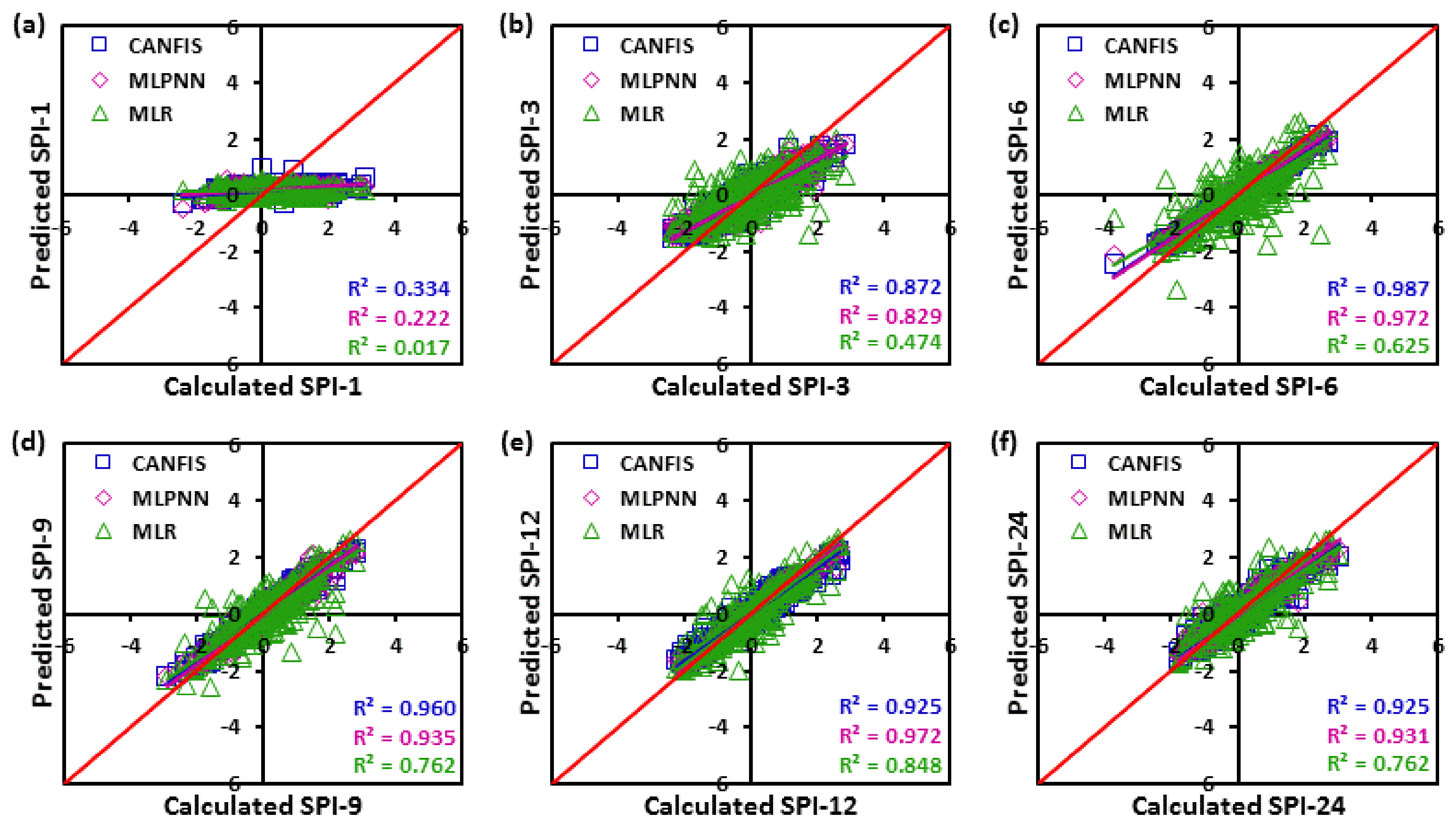
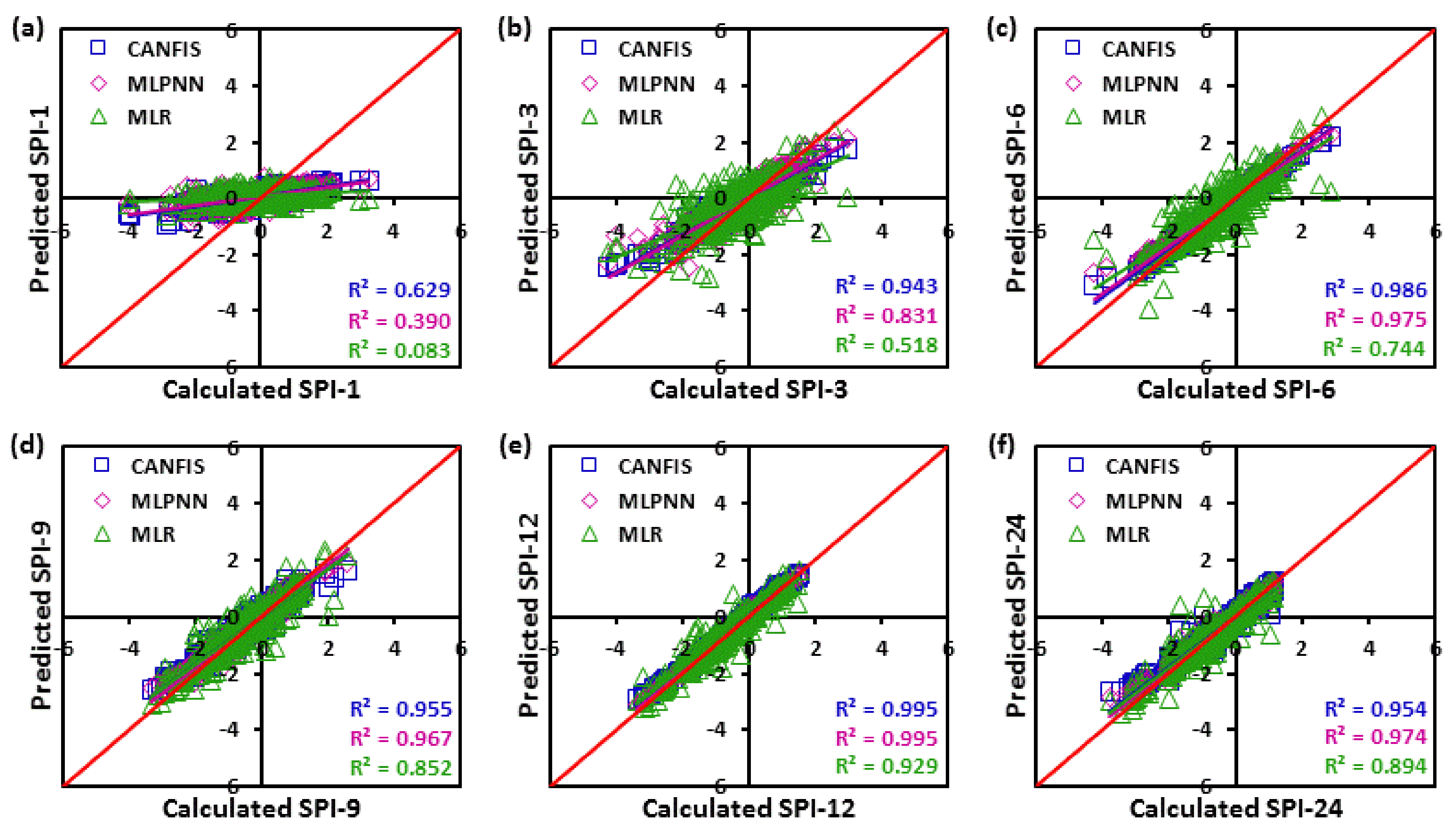
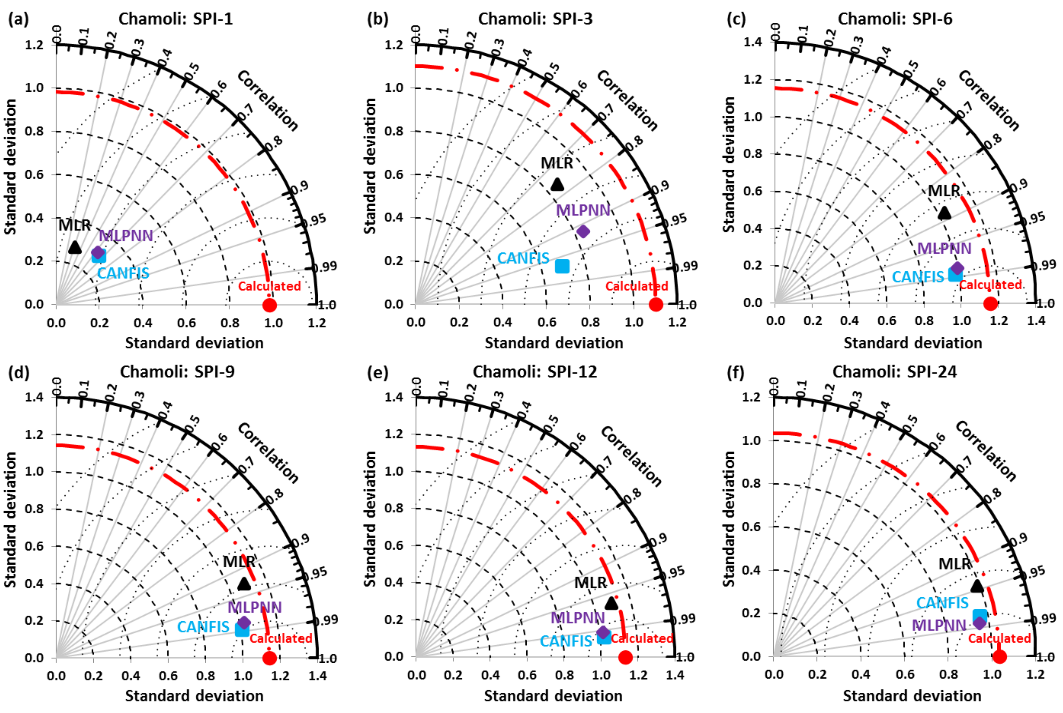
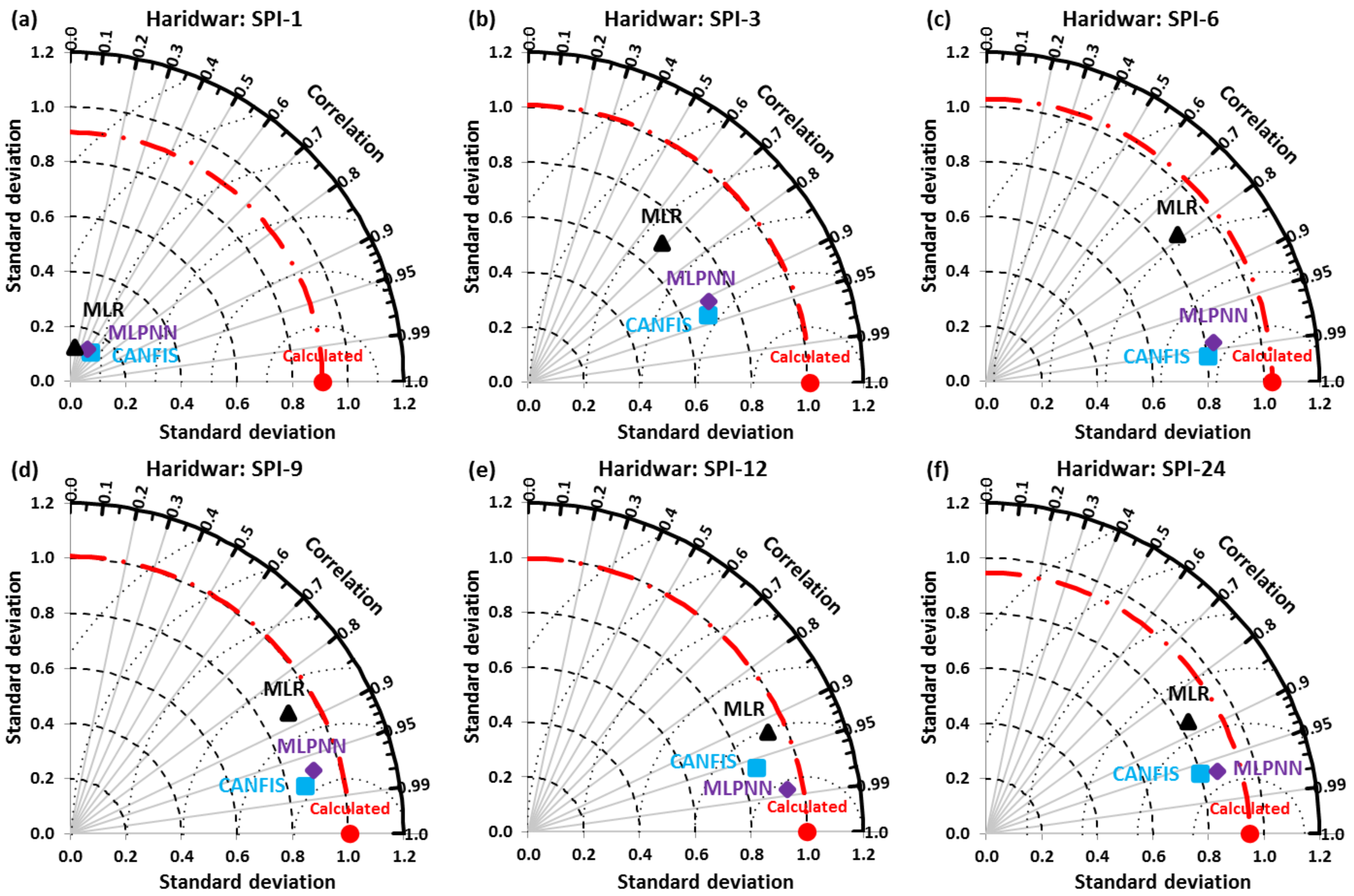
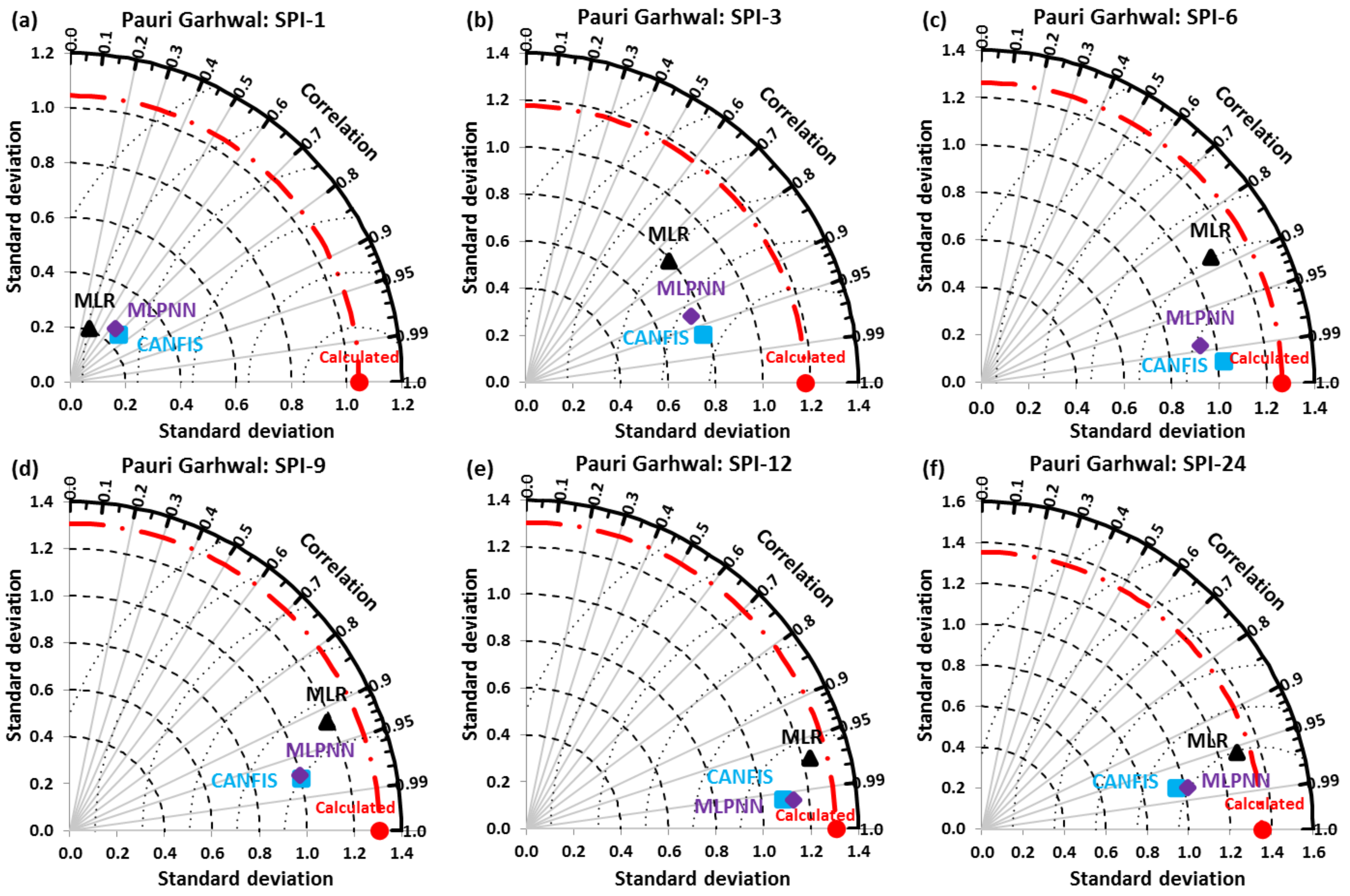
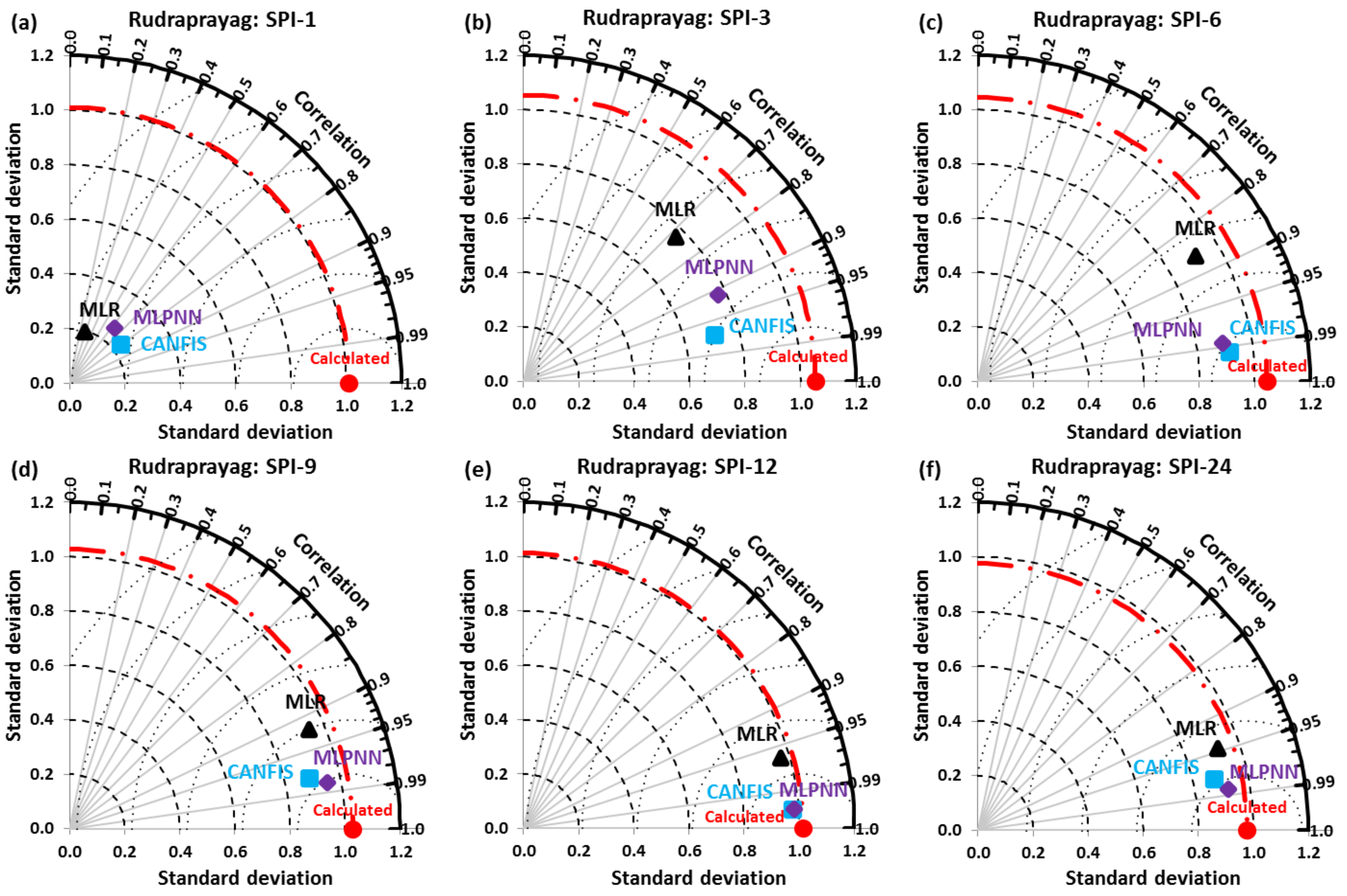
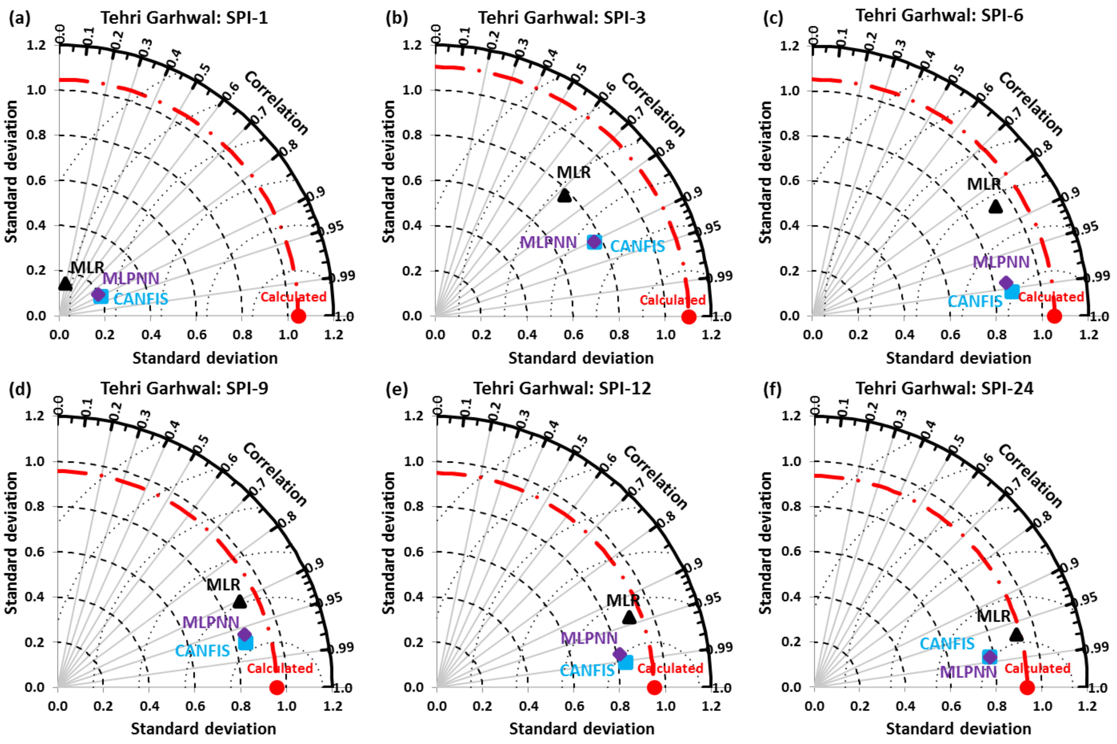
3.3. Performance Assessment by Using Scatter Plots and Taylor Diagram

The temporal disparity between the projected and computed (calculated) values for all SPI scales by the MLPNN, CANFIS, and MLR models during the testing span at Chamoli, Dehradun, Haridwar, Pauri Garhwal, Rudraprayag Tehri Garhwal, and Uttarkashi stations are presented in Figure 4, Figure 5, Figure 6, Figure 7, Figure 8, Figure 9 and Figure 10. As clearly seen from these figures, line of regression of CANFIS was quite near the best-fit line (highlighted by red color) for SPI-1, SPI-3, SPI-6, SPI-9, and SPI-12 at Chamoli and Tehri Garhwal; SPI-3, SPI-6, SPI-9, and SPI-12 at Dehradun; SPI-1, SPI-3, SPI-6, and SPI-9 at Haridwar and Pauri Garhwal; SPI-1, SPI-3, and SPI-6 at Rudraprayag; and SPI-3 at Uttarkashi. The MLPNN the regression line was close to the best-fit line on Chamoli and Tehri Garhwal for SPI-24; Dehradun for SPI-1 and SPI-24; Haridwar SPI-12 and SPI-24; Pauri Garhwal for SPI-12; Rudraprayag for SPI-9, SPI-12, and SPI-24; and Uttarkashi for SPI-1 and SPI-6. Likewise, for MLR models, these lines were close at Pauri Garhwal on SPI-24 and Uttarkashi on SPI-9, SPI-12, and SPI-24.

Accordingly, the spatial design of projected and calculated (observed) values of multi-scalar SPI for the MLPNN, CANFIS, and MLR models was also assessed by utilizing the Taylor diagram (TD) as a polar plot for attaining a graphical judgment of model performance based on SD, COC, and RMSE. Figure 11, Figure 12, Figure 13, Figure 14, Figure 15, Figure 16 and Figure 17 show the TD of MLPNN, CANFIS, and MLR models at Chamoli, Dehradun, Haridwar, Pauri Garhwal, Rudraprayag, Tehri Garhwal, and Uttarkashi, respectively, for the testing span. Consequently, Figure 11a–f shows that the CANFIS with chosen lags can be utilized for SPI projection at 1-, 3-, 6-, 9- and 12-month time spans, and MLPNN for the 24 months at Chamoli. Figure 12a–f displays that the CANFIS model with chosen lags can be utilized for SPI projection at 3-, 6-, 9- and 12-month time scales, and MLPNN for 1- and 24-month time spans at Dehradun. Figure 13a–f illustrates that the CANFIS model with certain lags can be utilized for SPI projection at 1-, 3-, 6-, and 9-month periods. The MLPNN model for 12-and 24-month time scales at Haridwar. Figure 14a–f demonstrates that the CANFIS model with certain lags was deployed for SPI projection at 1-, 3-, 6-, and 9-month time scales, MLPNN for the 12 months, and MLR the 24-month time scale at Pauri Garhwal. Figure 15a–f reveals that the CANFIS model with certain lags can be deployed for SPI projection at 1-, 3-, 6-month time scales and the MLPNN model for 9-, 12-, 24-month time spans at Rudraprayag. Figure 16a–f exposes that the CANFIS with certain lags can be utilized for SPI projection at 1-, 3-, 6-, 9-, and 12-month periods. The MLPNN model for 24 months at Tehri Garhwal. Figure 17a–f discloses that the CANFIS with certain lags can be utilized for SPI projection at 3-month time scales, MLR for 9-, 12-, 24-month duration, and MLPNN for 1- and 6-month duration at Uttarkashi.

4. Discussion

Table 4, Table 5 and Table 6 show that for a short time scale, i.e., SPI-1, both the AI and regression models yielded higher values of RMSE and lower values of NSE, COC, and WI. It means their unsatisfactory performance at a short time scale SPI. Apart from this, a comparison among AI performance (i.e., CANFIS and MLPNN) and regression (i.e., MLR) models is shown in

Table 7. Evaluation of AI and regression models at study stations.

Station	Index
	SPI-1	SPI-3	SPI-6	SPI-9	SPI-12	SPI-24
Chamoli	CANFIS	CANFIS	CANFIS	CANFIS	CANFIS	MLPNN
Dehradun	MLPNN	CANFIS	CANFIS	CANFIS	CANFIS	MLPNN
Haridwar	CANFIS	CANFIS	CANFIS	CANFIS	MLPNN	MLPNN
Pauri Garhwal	CANFIS	CANFIS	CANFIS	CANFIS	MLPNN	MLR
Rudraprayag	CANFIS	CANFIS	CANFIS	MLPNN	MLPNN	MLPNN
Tehri Garhwal	CANFIS	CANFIS	CANFIS	CANFIS	CANFIS	MLPNN
Uttarkashi	MLPNN	CANFIS	MLPNN	MLR	MLR	MLR

, which reveals that the CANFIS gained the highest-ranking followed by the MLPNN at all study sites except the Uttarkashi. Overall, the MLR model received a lower ranking at Chamoli, Dehradun, Haridwar, Pauri Garhwal, Rudraprayag, Tehri Garhwal stations, and the highest Uttarkashi station.

To make the results more concrete, this research’s findings were compared with the recent investigations conducted in different parts of the world on meteorological droughts’ prediction using stochastic and AI models. Mokhtarzad et al. [48] applied SVM, ANFIS, and ANN techniques to forecast the meteorological drought in Tehran based on SPI. According to the results, the SVM model provided more precise estimates than the ANFIS and ANN models. Nguyen et al. [49] conducted a study on the ANFIS model potential concerning meteorological drought prediction using SPEI and SPI at Khanhhoa Province, Vietnam. The investigation revealed the superior performance of the ANFIS model for SPEI and SPI in the study area. Zhang et al. [50] predicted the drought condition by employing the SVR, WANN, ANN, and ARIMA models that used 3 and 6 months of SPI values in Haihe River Basin, China. The estimated outcomes of SPI-6 and SPI-3 showed that the WANN model exhibited superior performance to other models. Liu et al. [51] used the Self-Adaptive Evolutionary-Extreme Learning Machine (SADE-ELM), Online Sequential-ELM (OS-ELM), and ELM for meteorological drought prediction based on SPEI and SPI in Khanhhoa Province, Vietnam. They found that the performance of the SADE-ELM models was superior to the other models. Mouatadid et al. [52] exploited the LSSVR, MLR, ANN, and ELM to forecast drought through various-scalar SPEI and SPI in eastern Australia. The results showed the better performance of ANN and ELM models than the LSSVR and MLR models. Özger et al. [53] applied standalone and hybrid use of ANFIS, SVM, and M5 models coupled with empirical mode decomposition (EMD-ANFIS, EMD-SVM, EMD-M5) and wavelet decomposition (i.e., WD-ANFIS, WD-SVM, WD-M5) for self-calibrated Palmer Drought Severity Index (SC-PDSI) prediction in the southern part of Turkey. The obtained results indicated the improved performance of hybrid WD-ANFIS, WD-SVM, and WD-M5 models over the other models. Considering the excellent performance of AI models, i.e., CANFIS and MLPNN, applied in this study, it might be insightful to compare these two models’ performances with other future studies models. In this regard, more recent meteorological data may be considered. Comparing two models applied in this study with other models for drought prediction to consider different climate projections would also be an essential task to be carried out in future studies to assist water managers in better long-term planning of water resources’ exploitation.

Accordingly, this study confirmed the superiority of AI models such as MLPNN and CANFIS in predicting meteorological droughts of various durations at the selected study stations.

5. Conclusions

This study analyzed the feasibility of AI and regression models that can be applied to predict the meteorological drought based on multi-scalar SPI at Pauri Garhwal, Chamoli, Rudraprayag, Dehradun, Haridwar, Uttarkashi, and Tehri Garhwal stations. Partial Autocorrelation Function (PACF) was utilized to choose the optimal input parameters (lags) for MLPNN, CANFIS, and MLR models at 5% significance level on SPI-24, SPI-12, SPI-9, SPI-6, SPI-3, and SPI-1 data series. The estimates yielded by the MLPNN, CANFIS, and MLR models were compared with the calculated (observed) values of multi-scalar SPI that applies statistical indicators, such as NSE, RMSE, WI, COC, and visual basis through Taylor diagram and scatter plot for study stations. Appraisal of results revealed that the applied AI models (i.e., CANFIS and MLPNN) significantly enhanced the modeling performance by improving the WI, COC, and NSE and decreasing the RMSE measurements in the study stations. Also, the executions of MLR at study stations were the poorest, except SPI-24 at Pauri Garhwal and SPI-9, SPI-12, and SPI-24 at Uttarkashi to predict meteorological drought. This study will help develop a reliable and standard intelligent system that can be used for the considered rainfall stations. It will be precious for policymakers and water resources managers to frame the study regions’ drought mitigation strategies.

References

1. Dracup, J.A.; Lee, K.S.; Paulson, E.G. On the statistical characteristics of drought events. Water Resour. Res. 1980, 16, 289–296. [Google Scholar] [CrossRef]
2. Wilhite, D.A.; Glantz, M.H. Understanding the drought phenomenon: The role of definitions. Water Int. 1985, 10, 111–120. [Google Scholar] [CrossRef] [Green Version]
3. Mishra, A.K.; Singh, V.P. Analysis of drought severity-area-frequency curves using a general circulation model and scenario uncertainty. J. Geophys. Res. 2009, 114, D06120. [Google Scholar] [CrossRef]
4. Mishra, A.K.; Singh, V.P. A review of drought concepts. J. Hydrol. 2010, 391, 202–216. [Google Scholar] [CrossRef]
5. Mishra, A.K.; Singh, V.P. Drought modeling—A review. J. Hydrol. 2011, 403, 157–175. [Google Scholar] [CrossRef]
6. McKee, T.B.; Doesken, N.J.; Kleist, J. The relationship of drought frequency and duration to time scales. In Proceedings of the Eighth Conference on Applied Climatology, Anaheim, CA, USA, 17–22 January 1993. [Google Scholar]
7. Mishra, A.K.; Desai, V.R. Drought forecasting using feed-forward recursive neural network. Ecol. Modell. 2006, 198, 127–138. [Google Scholar] [CrossRef]
8. Morid, S.; Smakhtin, V.; Bagherzadeh, K. Drought forecasting using artificial neural networks and time series of drought indices. Int. J. Climatol. 2007, 27, 2103–2111. [Google Scholar] [CrossRef]
9. Bacanli, U.G.; Firat, M.; Dikbas, F. Adaptive Neuro-Fuzzy Inference System for drought forecasting. Stoch. Environ. Res. Risk Assess. 2009, 23, 1143–1154. [Google Scholar] [CrossRef]
10. Belayneh, A.; Adamowski, J. Standard Precipitation Index Drought Forecasting Using Neural Networks, Wavelet Neural Networks, and Support Vector Regression. Appl. Comput. Intell. Soft Comput. 2012, 2012, 1–13. [Google Scholar] [CrossRef]
11. Özger, M.; Mishra, A.K.; Singh, V.P. Long Lead Time Drought Forecasting Using a Wavelet and Fuzzy Logic Combination Model: A Case Study in Texas. J. Hydrometeorol. 2012, 13, 284–297. [Google Scholar] [CrossRef]
12. Deo, R.C.; Şahin, M. Application of the Artificial Neural Network model for prediction of monthly Standardized Precipitation and Evapotranspiration Index using hydrometeorological parameters and climate indices in eastern Australia. Atmos. Res. 2015, 161–162, 65–81. [Google Scholar] [CrossRef]
13. Nguyen, L.B.; Li, Q.F.; Ngoc, T.A.; Hiramatsu, K. Adaptive Neuro-Fuzzy Inference System for drought forecasting in the Cai River basin in Vietnam. J. Fac. Agric. Kyushu Univ. 2015, 60, 405–415. [Google Scholar]
14. Djerbouai, S.; Souag-Gamane, D. Drought Forecasting Using Neural Networks, Wavelet Neural Networks, and Stochastic Models: Case of the Algerois Basin in North Algeria. Water Resour. Manag. 2016, 30, 2445–2464. [Google Scholar] [CrossRef]
15. Deo, R.C.; Tiwari, M.K.; Adamowski, J.F.; Quilty, J.M. Forecasting effective drought index using a wavelet extreme learning machine (W-ELM) model. Stoch. Environ. Res. Risk Assess. 2017, 31, 1211–1240. [Google Scholar] [CrossRef]
16. Komasi, M.; Sharghi, S.; Safavi, H.R. Wavelet and cuckoo search-support vector machine conjugation for drought forecasting using Standardized Precipitation Index (case study: Urmia Lake, Iran). J. Hydroinf. 2018, 20, 975–988. [Google Scholar] [CrossRef] [Green Version]
17. Abbasi, A.; Khalili, K.; Behmanesh, J.; Shirzad, A. Drought monitoring and prediction using SPEI index and gene expression programming model in the west of Urmia Lake. Theor. Appl. Climatol. 2019, 138, 553–567. [Google Scholar] [CrossRef]
18. Memarian, H.; Pourreza Bilondi, M.; Rezaei, M. Drought prediction using co-active neuro-fuzzy inference system, validation, and uncertainty analysis (case study: Birjand, Iran). Theor. Appl. Climatol. 2016, 125, 541–554. [Google Scholar] [CrossRef]
19. Rafiei-Sardooi, E.; Mohseni-Saravi, M.; Barkhori, S.; Azareh, A.; Choubin, B.; Jafari-Shalamzar, M. Drought modeling: A comparative study between time series and neuro-fuzzy approaches. Arab. J. Geosci. 2018, 11, 1–9. [Google Scholar] [CrossRef]
20. Malik, A.; Kumar, A.; Salih, S.Q.; Kim, S.; Kim, N.W.; Yaseen, Z.M.; Singh, V.P. Drought index prediction using advanced fuzzy logic model: Regional case study over Kumaon in India. PLoS ONE 2020, 15, e0233280. [Google Scholar] [CrossRef]
21. Guttman, N.B. Comparing the palmer drought index and the standardized precipitation index. J. Am. Water Resour. Assoc. 1998, 34, 113–121. [Google Scholar] [CrossRef]
22. Hayes, M.J.; Svoboda, M.D.; Wilhite, D.A.; Vanyarkho, O.V. Monitoring the 1996 Drought Using the Standardized Precipitation Index. Bull. Am. Meteorol. Soc. 1999, 80, 429–438. [Google Scholar] [CrossRef] [Green Version]
23. Angelidis, P.; Maris, F.; Kotsovinos, N.; Hrissanthou, V. Computation of Drought Index SPI with Alternative Distribution Functions. Water Resour. Manag. 2012, 26, 2453–2473. [Google Scholar] [CrossRef]
24. Yacoub, E.; Tayfur, G. Evaluation and Assessment of Meteorological Drought by Different Methods in Trarza Region, Mauritania. Water Resour. Manag. 2017, 31, 825–845. [Google Scholar] [CrossRef]
25. Lloyd-Hughes, B.; Saunders, M.A. A drought climatology for Europe. Int. J. Climatol. 2002, 22, 1571–1592. [Google Scholar] [CrossRef]
26. Mishra, A.K.; Desai, V.R. Spatial and temporal drought analysis in the Kansabati river basin, India. Int. J. River Basin Manag. 2005, 3, 31–41. [Google Scholar] [CrossRef]
27. Abramowitz, M.; Stegun, A. Handbook of Mathematical Formulas, Graphs, and Mathematical Tables; Dover Publishing: New York, NY, USA, 1965; p. 470. [Google Scholar]
28. Edwards, D.C.; McKee, T.B. Characteristics of 20th Century drought in the United States at multiple time scales. Atmos. Sci. Pap. 1997. [Google Scholar]
29. Jang, J.-S.R.; Sun, C.-T.; Mizutani, E. Neuro-Fuzzy and Soft Computing A Computational Approach to Learning and Machine Intelligence; Prentice Hall: Upper Saddle River, NJ, USA, 1997; ISBN 0132610663. [Google Scholar]
30. Malik, A.; Kumar, A. Pan Evaporation Simulation Based on Daily Meteorological Data Using Soft Computing Techniques and Multiple Linear Regression. Water Resour. Manag. 2015, 29, 1859–1872. [Google Scholar] [CrossRef]
31. Malik, A.; Kumar, A. Meteorological drought prediction using heuristic approaches based on effective drought index: A case study in Uttarakhand. Arab. J. Geosci. 2020, 13, 1–17. [Google Scholar] [CrossRef]
32. Malik, A.; Kumar, A.; Piri, J. Daily suspended sediment concentration simulation using hydrological data of Pranhita River Basin, India. Comput. Electron. Agric. 2017, 138, 20–28. [Google Scholar] [CrossRef]
33. Malik, A.; Kumar, A.; Kisi, O. Monthly pan-evaporation estimation in Indian central Himalayas using different heuristic approaches and climate based models. Comput. Electron. Agric. 2017, 143, 302–313. [Google Scholar] [CrossRef]
34. Singh, A.; Malik, A.; Kumar, A.; Kisi, O. Rainfall-runoff modeling in hilly watershed using heuristic approaches with gamma test. Arab. J. Geosci. 2018, 11, 1–12. [Google Scholar] [CrossRef]
35. Sugeno, M.; Kang, G. Structure identification of fuzzy model. Fuzzy Sets Syst. 1988, 28, 15–33. [Google Scholar] [CrossRef]
36. Takagi, T.; Sugeno, M. Fuzzy identification of systems and its applications to modeling and control. IEEE Trans. Syst. Man. Cybern. 1985, SMC-15, 116–132. [Google Scholar] [CrossRef]
37. Aytek, A. Co-active neurofuzzy inference system for evapotranspiration modeling. Soft Comput. 2009, 13, 691–700. [Google Scholar] [CrossRef]
38. Tabari, H.; Talaee, P.H.; Abghari, H. Utility of coactive neuro-fuzzy inference system for pan evaporation modeling in comparison with multilayer perceptron. Meteorol. Atmos. Phys. 2012, 116, 147–154. [Google Scholar] [CrossRef]
39. Haykin, S. Neural Networks—A Comprehensive Foundation, 2nd ed.; Prentice-Hall International, Inc.: Upper Saddle River, NJ, USA, 1999; pp. 26–32. [Google Scholar]
40. Dawson, C.W.; Wilby, R.L. Hydrological modelling using artificial neural networks. Prog. Phys. Geogr. Earth Environ. 2001, 25, 80–108. [Google Scholar] [CrossRef]
41. Landeras, G.; Ortiz-Barredo, A.; López, J.J. Forecasting Weekly Evapotranspiration with ARIMA and Artificial Neural Network Models. J. Irrig. Drain. Eng. 2009, 135, 323–334. [Google Scholar] [CrossRef]
42. Deo, R.C.; Kisi, O.; Singh, V.P. Drought forecasting in eastern Australia using multivariate adaptive regression spline, least square support vector machine and M5Tree model. Atmos. Res. 2017, 184, 149–175. [Google Scholar] [CrossRef] [Green Version]
43. Douglas, E.M.; Vogel, R.M.; Kroll, C.N. Trends in floods and low flows in the United States: Impact of spatial correlation. J. Hydrol. 2000, 240, 90–105. [Google Scholar] [CrossRef]
44. Nash, J.E.; Sutcliffe, J.V. River flow forecasting through conceptual models part I—A discussion of principles. J. Hydrol. 1970, 10, 282–290. [Google Scholar] [CrossRef]
45. Moriasi, D.N.; Gitau, M.W.; Pai, N.; Daggupati, P. Hydrologic and Water Quality Models: Performance Measures and Evaluation Criteria. Trans. ASABE 2015, 58, 1763–1785. [Google Scholar]
46. Willmott, C.J. On the validation of models. Phys. Geogr. 1981, 2, 184–194. [Google Scholar] [CrossRef]
47. Taylor, K.E. Summarizing multiple aspects of model performance in a single diagram. J. Geophys. Res. Atmos. 2001, 106, 7183–7192. [Google Scholar] [CrossRef]
48. Mokhtarzad, M.; Eskandari, F.; Jamshidi Vanjani, N.; Arabasadi, A. Drought forecasting by ANN, ANFIS, and SVM and comparison of the models. Environ. Earth Sci. 2017, 76, 729. [Google Scholar] [CrossRef]
49. Nguyen, V.; Li, Q.; Nguyen, L. Drought forecasting using ANFIS- a case study in drought prone area of Vietnam. Paddy Water Environ. 2017, 15, 605–616. [Google Scholar] [CrossRef]
50. Zhang, Y.; Li, W.; Chen, Q.; Pu, X.; Xiang, L. Multi-models for SPI drought forecasting in the north of Haihe River Basin, China. Stoch. Environ. Res. Risk Assess. 2017, 31, 2471–2481. [Google Scholar] [CrossRef]
51. Liu, Z.; Li, Q.; Nguyen, L.; Xu, G. Comparing Machine-Learning Models for Drought Forecasting in Vietnam’s Cai River Basin. Pol. J. Environ. Stud. 2018, 27, 2633–2646. [Google Scholar] [CrossRef] [Green Version]
52. Mouatadid, S.; Raj, N.; Deo, R.C.; Adamowski, J.F. Input selection and data-driven model performance optimization to predict the Standardized Precipitation and Evaporation Index in a drought-prone region. Atmos. Res. 2018, 212, 130–149. [Google Scholar] [CrossRef]
53. Özger, M.; Başakın, E.E.; Ekmekcioğlu, Ö.; Hacısüleyman, V. Comparison of wavelet and empirical mode decomposition hybrid models in drought prediction. Comput. Electron. Agric. 2020, 179, 105851. [Google Scholar] [CrossRef]
Figure 1. Location map of Garhwal region with seven meteorological stations.
Climate 09 00028 g001
Figure 3. Three-layer multi-layer perceptron neural network (MLPNN) model configuration.
Climate 09 00028 g003
Figure 4. (af) Scatter plots of calculated and predicted multi-scalar SPI values by CANFIS, MLPNN, and MLR models during the testing period at Chamoli station.
Climate 09 00028 g004
Figure 5. (af) Scatter plots of calculated and predicted multi-scalar SPI values by CANFIS, MLPNN, and MLR models during the testing period at Dehradun station.
Climate 09 00028 g005
Figure 6. (af) Scatter plots of calculated and predicted multi-scalar SPI values by CANFIS, MLPNN, and MLR models during the testing period at Haridwar station.
Climate 09 00028 g006
Figure 7. (af) Scatter plots of calculated and predicted multi-scalar SPI values by CANFIS, MLPNN, and MLR models during the testing period Pauri Garhwal station.
Climate 09 00028 g007
Figure 8. (af) Scatter plots of calculated and predicted multi-scalar SPI values by CANFIS, MLPNN, and MLR models during the testing period at Rudraprayag station.
Climate 09 00028 g008
Figure 9. (af) Scatter plots of calculated and predicted multi-scalar SPI values by CANFIS, MLPNN, and MLR models during the Tehri Garhwal station’s testing period.
Climate 09 00028 g009
Figure 10. (af) Scatter plots of calculated and predicted multi-scalar SPI values by CANFIS, MLPNN, and MLR models during the testing period at Uttarkashi station.
Climate 09 00028 g010
Figure 11. (af) Taylor diagram of predicted and calculated multi-scalar SPI at Chamoli station.
Climate 09 00028 g011
Figure 12. (af) Taylor diagram of predicted and calculated multi-scalar SPI at Dehradun station.
Climate 09 00028 g012
Figure 13. (af) Taylor diagram of predicted and calculated multi-scalar SPI at Haridwar station.
Climate 09 00028 g013
Figure 14. (af) Taylor diagram of predicted and calculated multi-scalar SPI at Pauri Garhwal station.
Climate 09 00028 g014
Figure 15. (af) Taylor diagram of predicted and calculated multi-scalar SPI at Rudraprayag station.
Climate 09 00028 g015
Figure 16. (af) Taylor diagram of predicted and calculated multi-scalar SPI at Tehri Garhwal station.
Climate 09 00028 g016
Figure 17. (af) Taylor diagram of predicted and calculated multi-scalar SPI at Uttarkashi station.
Climate 09 00028 g017