Article

Evaluation of Climate Change on Streamflow, Sediment, and Nutrient Load at Watershed Scale

1
Department of Agricultural and Biological Engineering, Mississippi State University, Starkville, MS 39762, USA
2
Department of Ecology and Conservation Biology, Texas A&M University, College Station, TX 77843, USA
*
Author to whom correspondence should be addressed.
Climate 2021, 9(11), 165; https://doi.org/10.3390/cli9110165
Submission received: 15 September 2021 / Revised: 21 October 2021 / Accepted: 3 November 2021 / Published: 7 November 2021

Abstract

:
This study evaluated changes in climatic variable impacts on hydrology and water quality in Big Sunflower River Watershed (BSRW), Mississippi. Site-specific future time-series precipitation, temperature, and solar radiation data were generated using a stochastic weather generator LARS-WG model. For the generation of climate scenarios, Representative Concentration Pathways (RCPs), 4.5 and 8.5 of Global Circulation Models (GCMs): Hadley Center Global Environmental Model (HadGEM) and EC-EARTH, for three (2021–2040, 2041–2060 and 2061–2080) future climate periods. Analysis of future climate data based on six ground weather stations located within BSRW showed that the minimum temperature ranged from 11.9 °C to 15.9 °C and the maximum temperature ranged from 23.2 °C to 28.3 °C. Similarly, the average daily rainfall ranged from 3.6 mm to 4.3 mm. Analysis of changes in monthly average maximum/minimum temperature showed that January had the maximum increment and July/August had a minimum increment in monthly average temperature. Similarly, maximum increase in monthly average rainfall was observed during May and maximum decrease was observed during September. The average monthly streamflow, sediment, TN, and TP loads under different climate scenarios varied significantly. The change in average TN and TP loads due to climate change were observed to be very high compared to the change in streamflow and sediment load. The monthly average nutrient load under two different RCP scenarios varied greatly from as low as 63% to as high as 184%, compared to the current monthly nutrient load. The change in hydrology and water quality was mainly attributed to changes in surface temperature, precipitation, and stream flow. This study can be useful in the development and implementation of climate change smart management of agricultural watersheds.

1. Introduction

The global surface temperature has been increasing at the rate of 0.2 °C per decade as a result of greenhouse gas emissions in the past and present [1,2] Heavy precipitation has been observed in some regions of the world while other parts of the world have observed deficit precipitation drought [1] Such variation in the global temperature precipitation pattern is an indicator of climate change which increases the risk of environmental hazards such as flooding storm surge landslides soil erosion, d.r.o.u.g.h.t.; other environmental damage [3] Hydrologists are more concerned about climate change since it has a significant effect on water resources hydrological, p.r.o.c.e.s.s.e.s. Climate change assessment is a major part of water resource management for any project. The climate change impact study related to hydrology and water quality of specific watershed characteristics may vary from general to macro scale [4]. Climate change assessment can be performed based on climate change scenario data obtained from different sources such as General Circulations Models (GCMs). GCMs have been developed for the generation of future climate data for any part of the globe. Although they are available for any part of the world, these data may not be used directly at study sites because of their coarse spatial resolution [5].
Among various approaches to the climate change impact assessment on hydrology, such as water quality, crop yield, soil erosion etc., the application of hydrological models is the most effective method [6,7,8,9]. A hydrologic and water quality model, Soil and Water Assessment Tool (SWAT) has been extensively used to analyse the impact of climate change on hydrology and water quality by incorporating the climate data on the model [9,10,11]. The finer resolution climate data, as required by the models can be prepared by downscaling the output of GCM climate data. The hydrologic and water quality simulation of the models for different climate scenarios can be compared with the base scenario using ground stations weather data of the current period.
Limited climate change assessment studies on streamflow, sediment, and crop yield have been carried out in the south-eastern U.S. including within the Big Sunflower River Watershed (BSRW) and the Mississippi watersheds in the past. However, the assessment of the impact of climate change on nutrient load has not yet been conducted for the BSRW, which is essential to improve the water quality and agroecosystem, including the hypoxia at the Gulf-of Mexico, where Big Sunflower River contributes as a tributary. The objectives of this study were to: (a) analyse the changes in climatic variables: precipitation and temperatures, and (b) evaluate the impact of climate change on streamflow, sediment, TN, and TP loads using SWAT for every 20 years from 2021 to 2080 for RCP scenarios, RCP 4.5, and RCP 8.5 of the Global Circulation Models (GCMs), HadGEM2, and EC-Earth.

2. Methods and Methodology
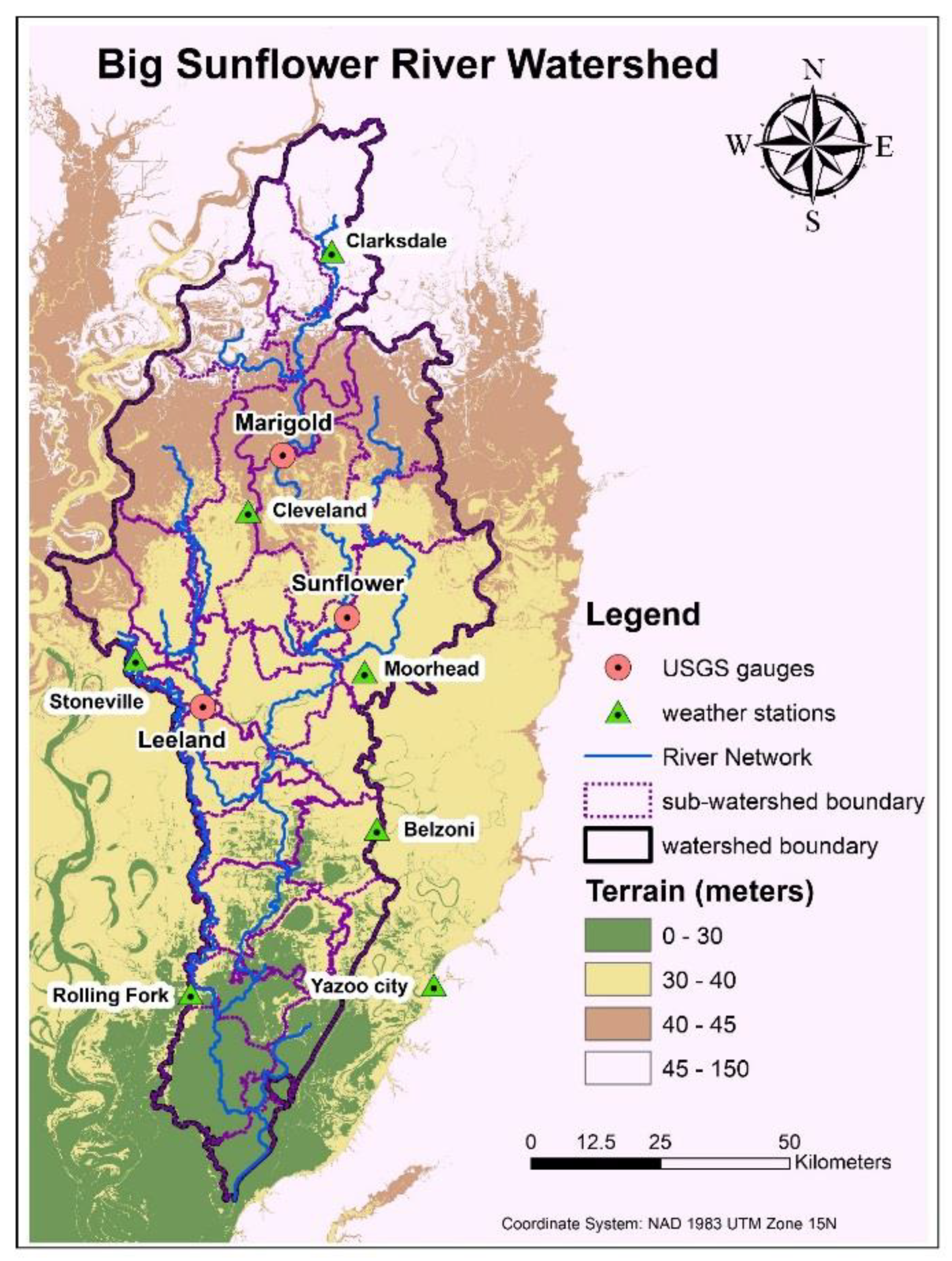
2.1. Study Area

The BSRW, an agricultural watershed located at the north-western part of the state of Mississippi in the conterminous United States, was selected as a study area to analyze climate change and its impact on hydrology and water quality. The BSRW is located between latitude: 32°30′ N to 34°25′ N and longitude: 91°10′ E to 90°13′ E. There is little variation in elevation as the watershed is dominated by the plain area, having a slope less than 3%. Watershed covers a drainage area of about 10,500 km2, with about 75% cropland, 15% forest/wetlands, and 10% urban/other areas. Weather variables obtained from the six ground weather stations located at Belzoni, Clarksdale, Greenville, Moorhead, Rolling Fork, and Yazoo within BSRW were used for the climate change analysis. The location of BSRW, along with its sub-watersheds, river network, USGS gauges, and weather stations, is presented in Figure 1.

2.2. Data

Climate change scenario data on precipitation, surface temperature (maximum and minimum), and solar radiation were obtained for two GCMs, HadGEM and EC-EARTH, of the IPCC Coupled Model Intercomparison Project- phase 5 (CMIP5) [12]. A stochastic weather generator, Long Ashton Research Station Weather Generator (LARS-WG), was used to develop climate change scenarios for six ground weather stations within the BSRW, as shown in Figure 1. The two different anticipated greenhouse concentration trajectories, also known as Representative concentration pathways (RCPs), RCP 4.5 and RCP 8.5, were considered in this study, since these two RCPs can effectively reflect future climate change following the present climate condition and have been applied by other studies [13,14,15,16]. Climate change analysis for six ground weather stations located within the BSRW was performed based on the two RCP scenarios, RCP 4.5 and RCP 8.5, of GCM models: HadGEM2, and EC Earth.

2.3. LARS-WG

The LARS-WG is a stochastic weather generator, a downscaling tool that can be used in the generation of local-scale climate scenarios based on global or regional climate models [17]. The LARS-WG can be used to generate site-specific future climate time-series of precipitation, maximum and minimum temperature, and solar radiation data from observed weather data using the semi-empirical distribution method defined as a cumulative probability distribution [18,19]. The LARS-WG has a large number of parameters and thus it requires a longer time-series of weather data, generally greater than 20 to 30 years, for parameterization. In addition to the observed time-series of weather data for a specific station, a file containing site information as station-name, latitude, longitude, and altitude of the station is also required for the generation of climate data using the LARS-WG model. This model has been validated for diverse climates around the world and computes a set of parameters for probability distributions of weather variables with the help of observed daily weather time-series for each site that are used to generate synthetic weather time series of random length [19]. In addition to the generation of climate time-series data, it also performs a different statistical test to compare probability distribution of observed and synthetic climate data, their mean and standard deviations. In this study, three tests: chi-square test, t-test, and F-test, at 5% significance level, were used to compare the goodness of fit, means, and standard deviations of observed and synthetic data. This weather generator has also been used in previous climate change assessment studies at the BSRW [18,20,21].

2.4. SWAT

The SWAT model is a physically based, semi-distributed, and continuous-simulating model operating on daily time step [22]. The SWAT model is primarily used to simulate the impact of land management on water, sediment, nutrients, and crop yield in a watershed of various size, topography, soil types and land use conditions [23,24]. This model is one of the most suitable models for the study on hydrology, sediment, and nutrient load [25,26] from agricultural watersheds. Apart from the simulation of hydrology, water quality, and the effect of agricultural land management practices on water, it can also be used to simulate the effect of climate change on hydrology and water quality [9,10,11]. ArcSWAT interface was used in this study to analyze the effect of climate data on streamflow, sediment, TN, and TP load. ArcSWAT takes the input of the Digital Elevation Model (DEM) to delineate a watershed and divide it into several sub-watersheds, which are further divided into Hydrologic Response Units (HRUs) with the addition of inputs: soil and land-use/land-cover data layer. HRU is the smallest spatial unit in the model, having similar elevation, soil type, and land-use/land-cover class. ArcSWAT also requires daily weather timeseries data such as precipitation, maximum and minimum temperature, and solar radiation, along with agricultural management data for the simulation.
Calibrated SWAT model for the BSRW was recalibrated and revalidated using the Sequential Uncertainty Fitting (SUFI-2) procedure inside the SWAT autocalibration tool: SWAT Calibration and Uncertainty Procedures (SWAT-CUP) for flow, sediment, TN, and TP using observed data at three USGS gauging stations. To access the performance of the model, the statistics Nash–Sutcliffe Efficiency (NSE) and the coefficient of determination (R2) were used.

3. Result and Discussion

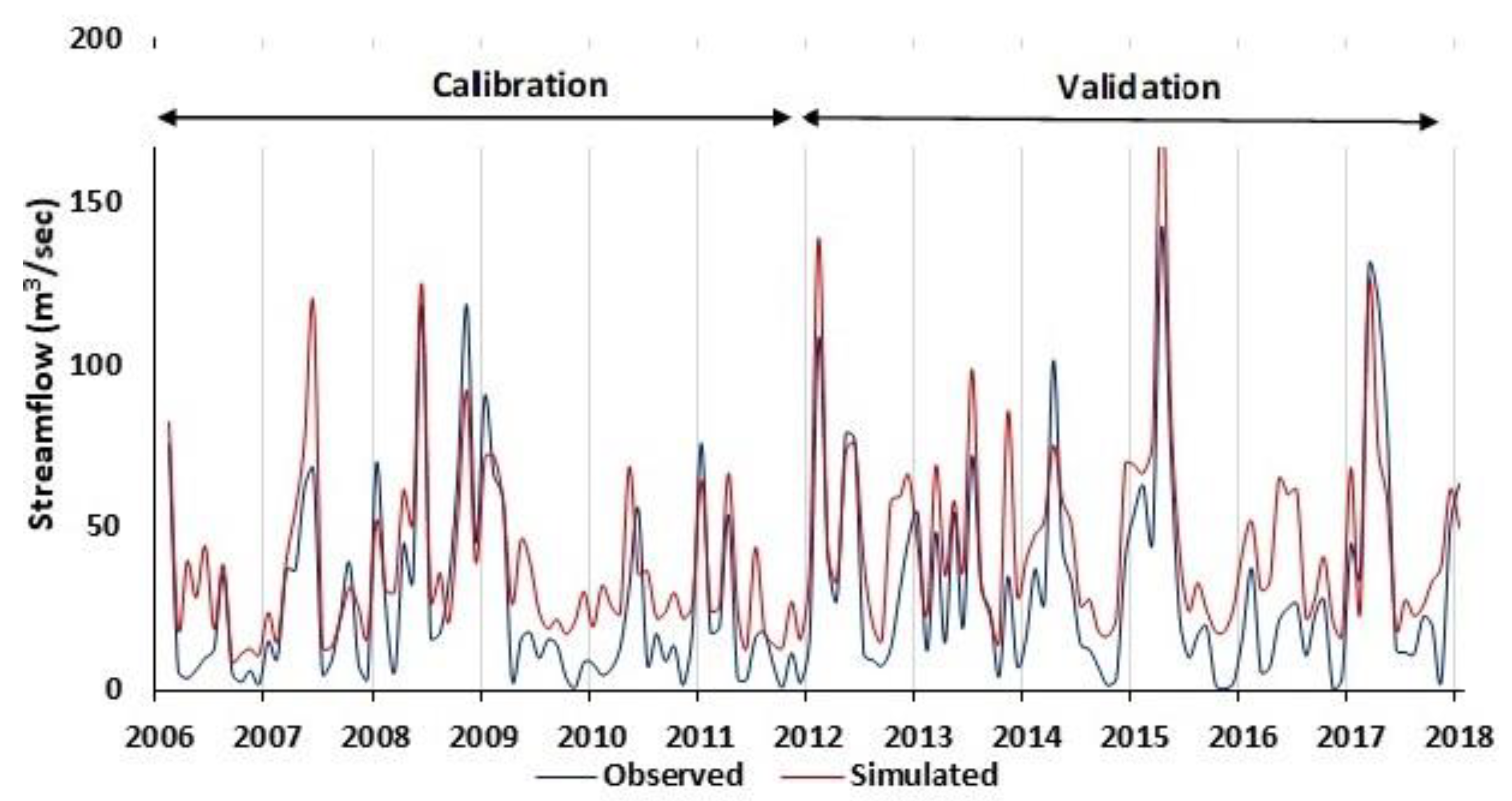
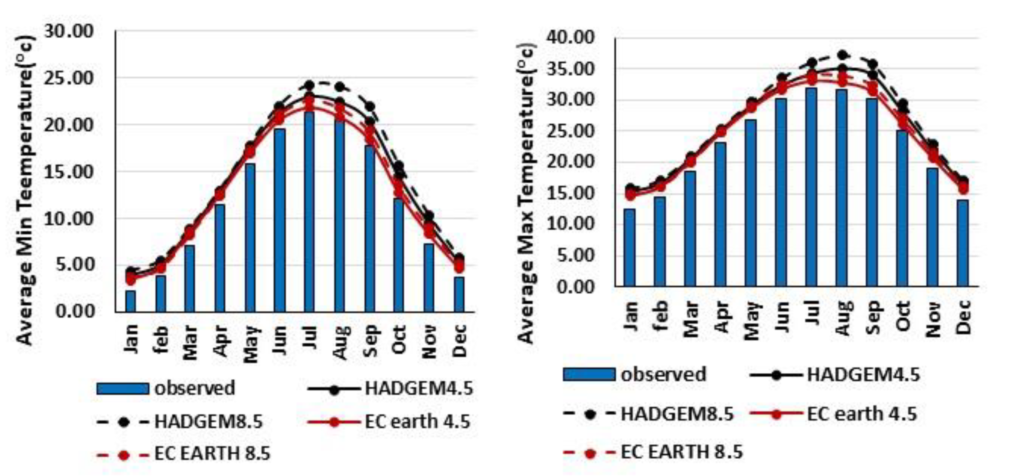
3.1. SWAT Model Recalibration and Revalidation

Calibrated SWAT for the BSRW [27] was recalibrated for streamflow using the monthly flow data from 2006 to 2012 and revalidated from 2013 to 2018 at three USGS gauge stations (Marigold, Sunflower, Leland). Similarly, sediment, TN, and TP load were recalibrated and revalidated from 2014 to 2015 and 2015 to 2016 respectively, using the biweekly water quality data obtained from the three USGS gauge stations. The comparison of observed and simulated streamflow at sunflower gauge station from 2007 to 2018 is presented in Figure 2 and the summary of statistics for recalibration/revalidation of SWAT for streamflow, sediment, TN, and TP load from three gauge stations within BSRW is presented in Table 1.

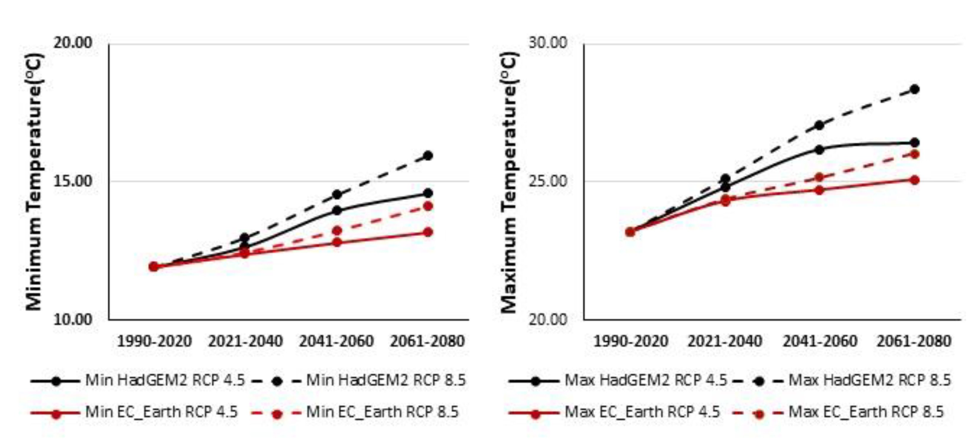
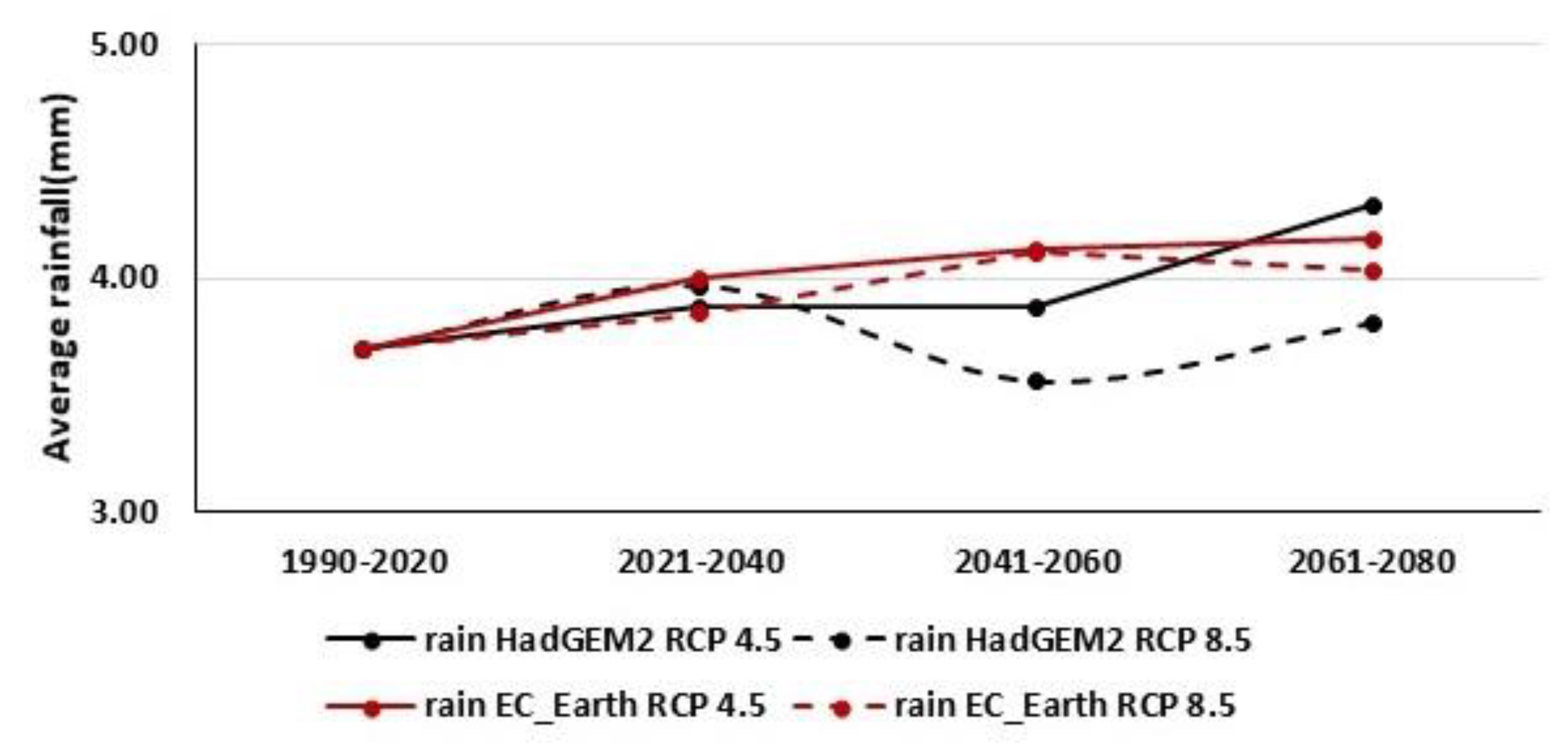
3.2. Climate Change Analysis

Climate change analysis based on climate change scenarios for six ground weather stations located in the BSRW showed that average minimum temperature for six ground weather stations ranged from 12.4 °C to 13 °C during 2021 to 2040, 12.8 °C to 14.5 °C during 2041 to 2060, and 13.2 °C to 15.9 °C during 2061 to 2080 for two different RCP scenarios of two different models. Similarly average maximum temperature ranged from 24.3 °C to 25.1 °C during 2021 to 2040, 24.7 °C to 27.1 °C during 2041 to 2060, and 25.1 °C to 28.3 °C during 2061 to 2080. RCP 8.5 of HadGEM2 model showed the highest percentage increase in minimum and maximum temperature. Change in average maximum and minimum temperature for 2021–2040, 2041–2060 and 2061 to 2080 for climate scenarios, RCP 4.5, and RCP 8.5 of GCM models, HadGEM2, and EC-Earth are presented in Figure 3.
Similarly, average rainfall during the period of 2021 to 2040 increased by 8% for RCP 4.5 of EC-Earth models, while the increase in average rainfall amount was 4% for RCP 8.5 of the same model. RCP 8.5 of the HadGEM2 model observed a decrease in average precipitation by 11% from 2041 to 2061 and RCP 8.5 of EC Earth observed a decrease in average precipitation by 2% during 2061 to 2080. Changes in average daily rainfall for 2021–2040, 2041–2060 and 2061 to 2080 for climate change scenarios, RCP 4.5, and RCP 8.5 of GCM models, HadGEM2, and EC-Earth are presented in Figure 4.
The summary of the change in average minimum and maximum and average rainfall for six ground weather stations during the period of 2021 to 2040, 2041 to 2060 and 2061 to 2080 for climate scenarios, RCP 4.5 and RCP 8.5 of GCM models, HadGEM2 and EC-Earth is presented in Table 2.
The monthly average of the maximum and minimum temperature was observed to increase for both RCP scenarios: RCP 4.5 and RCP 8.5 of models HadGEM2 and EC-Earth. Increases in minimum and maximum temperature were the highest during January, while they were the lowest from May to August. The projected average minimum temperature for January was 4.3 °C according to RCP 8.5 of the HadGEM2 model and 3.9 °C according to RCP 4.5 of the same model. The projected average minimum temperature for August according to RCP 4.5 and RCP 8.5 of the EC-Earth model was 20.8 °C and 21.8 °C, respectively.
In the same way, the projected average maximum temperature for January was 15.8 °C and 15.2 °C according to RCP 8.5 and RCP 4.5 of the HadGEM2 model. Projected average maximum temperature for July according to RCP 4.5 and RCP 8.5 of the EC-Earth model were 33.1 °C and 33.9 °C, respectively. Average monthly maximum and minimum temperatures for climate scenarios RCP 4.5 and RCP 8.5 of the GCM models, HadGEM2 and EC-Earth, along with observed monthly maximum and minimum temperatures, are presented in Figure 5.
The monthly average observed precipitation data were compared with climate scenarios: RCP 4.5 and RCP 8.5 of models HadGEM2 and EC-Earth. Average rainfall increased by 32% and 24% in May according to RCP 4.5 and 8.5 of the HadGEM2 model, while average rainfall decreased by 22% and 31% in September according to RCP 4.5 and 8.5 of the HadGEM2 model. Similarly, average rainfall increased by 34% in August and 21% in May according to RCP 4.5 and 8.5 of the EC-Earth model, while average rainfall decreased by 7% in December and 5% in September according to RCP 4.5 and 8.5 of the EC-Earth model.

3.3. Climate Change Impact on Hydrology and Water Quality

The impact of climate change on hydrology and water quality was assessed using the output from the SWAT model after incorporating weather data from RCP 4.5 and RCP 8.5 of the GCMs, HadGEM and EC-EARTH. Average monthly streamflow, sediment yield, TN, and TP load for three different monitoring stations were evaluated for different climate scenarios and the changes in their monthly average outputs as compared to observed values.

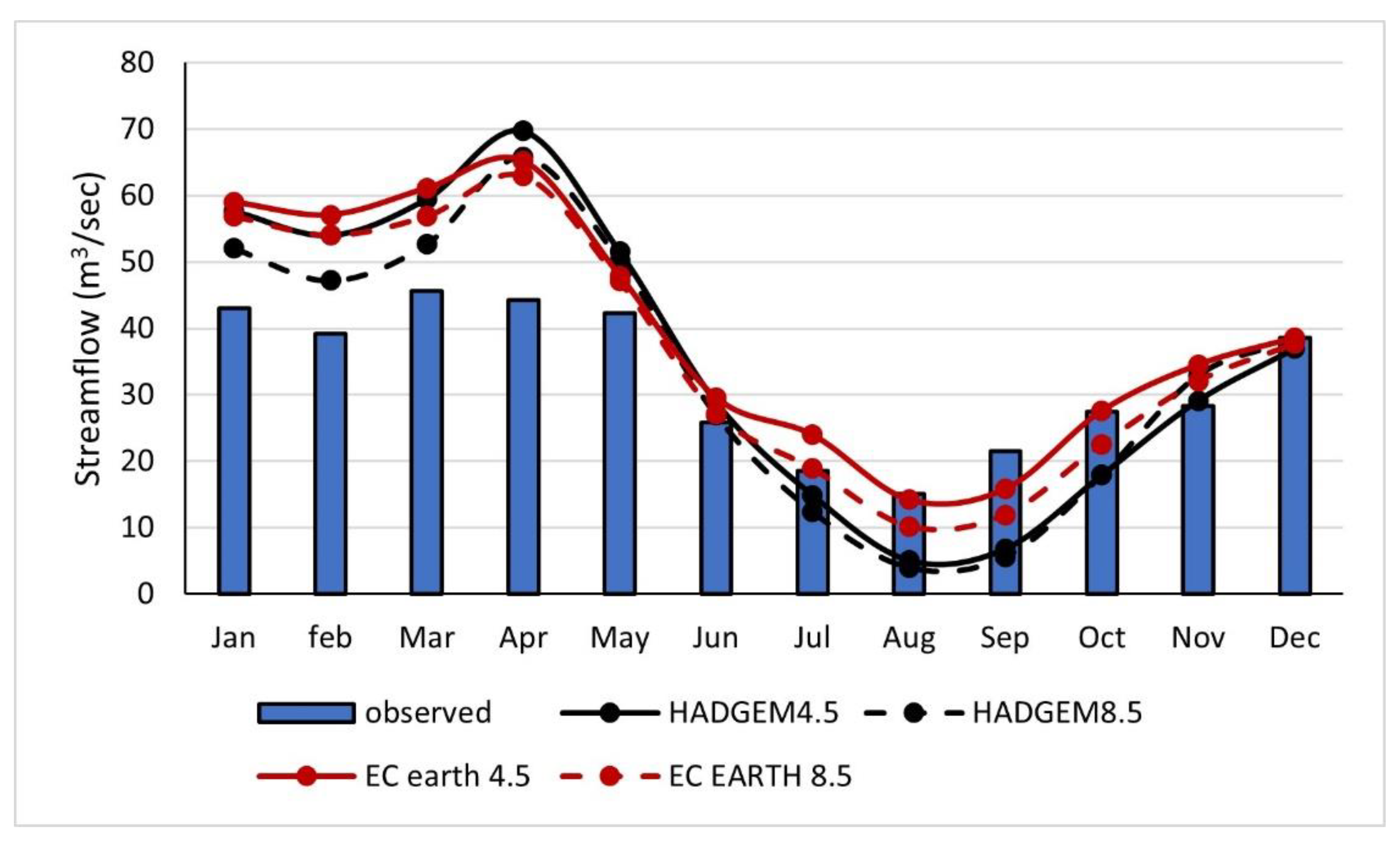
3.3.1. Climate Change Impact on Streamflow

The change in average streamflow for the 2021 to 2040 climate period increased by 5% to 19%, while the change in average streamflow for 2041–2060 decreased by 19% or increased up to 13%, and that for 2061 to 2080 was decreased by 3% or increased up to 17%. Similarly, the average monthly streamflow was predicted maximum during April for the HadGEM2 (RCP 4.5 and RCP8.5) model. The average monthly streamflow was predicted maximum during January for the EC-Earth model. Summary of the percentage change in streamflow during the period of 2021 to 2040, 2041 to 2060 and 2061 to 2080 for climate scenarios, RCP 4.5 and RCP 8.5 of GCM models, HadGEM2 and EC-Earth are presented in Table 3.
Monthly average streamflow as predicted by SWAT model based on climate change scenarios were compared with the observed monthly average streamflow data. Average monthly streamflow found the highest during April and lowest during August under both climate scenarios of both models, while observed streamflow determined the highest in March and lowest in August. The monthly average streamflow predicted to be increased or decreased during the year based on GCM model and RCP climate scenarios. Average streamflow was increased by 57% and 49% in April according to RCP 4.5 and 8.5 of the HadGEM2 model and by 47% and 42% according to RCP 4.5 and 8.5 of EC-Earth model, respectively. Similarly, average streamflow was decreased by 68% and 74% in September according to RCP 4.5 and 8.5 of HadGEM2 model and by 27% and 45% according to RCP 4.5 and 8.5 of EC-Earth model, respectively. The average monthly streamflow under climate scenarios RCP 4.5 and RCP 8.5 of the GCM models HadGEM2 and EC- Earth are given in Figure 6.
Application of climate data on the SWAT model showed a higher amount of streamflow for March to May with the peak in April. Extreme precipitation events are likely to increase during these months, which is the main cause of streamflow rise [28].

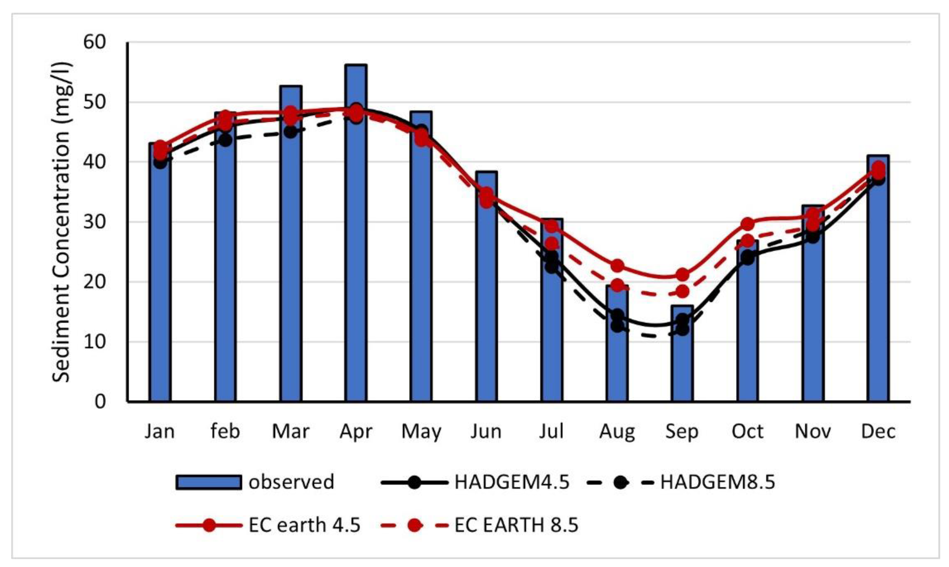
3.3.2. Climate Change Impact on Sediment Concentration

Model simulated average sediment concentration for the period of 2021 to 2040 time period found decreased from 3% to 12%, while the change in average sediment concentration for 2041–2060 time period was decreased by 14% or increased by 4%, and that for 2061 to 2080 time period decreased by 1% or increased by 7%. Likewise, average monthly sediment concentration was maximum during the month of April for both the climate change scenarios (RCP 4.5 and RCP 8.5) of both models (HadGEM2 and EC-Earth). The summary of the percentage change in sediment concentration during the period of 2021 to 2040, 2041 to 2060 and 2061 to 2080 for climate scenarios, RCP 4.5 and RCP 8.5 of the GCM models, HadGEM2 and EC-Earth are presented in Table 4.
Monthly average sediment concentration as predicted by SWAT model based on climate change scenarios were compared with the observed monthly average sediment concentration data. The observed monthly sediment concentration and average monthly sediment concentration under both climate scenarios of both models determined the highest during April and found the lowest during September. The monthly average sediment concentration that increased or decreased during the year were based on climate scenarios and the selection of models. Average decrease in sediment concentration according to RCP 4.5 and RCP 8.5 of the HadGEM2 model was 5% and 7%, respectively, in January, 13% and 16% in April, 20% and 26% in July and 25% and 35% in August. On the other hand, average sediment concentration was increased by 33% and 15%, respectively in September and 17% and 0.3%, respectively, in August according to RCP 4.5 and 8.5 of the EC-Earth model, while average sediment concentration was decreased by 14% and 15%, respectively, in April and by 8% to 10% in May according to RCP 4.5 and RCP 8.5 of the EC-Earth model. Average monthly sediment concentration under climate scenarios RCP 4.5 and RCP 8.5 of GCM models: HadGEM2 and EC-Earth are given in Figure 7.
The SWAT simulated model outputs based on all climate change scenarios showed that sediment concentration in April were considerably low compared to the observed monthly sediment concentration. Although, sediment concentration prediction is related to streamflow, the relation is not always linear [29,30]. The sediment concentration was not only dependent on discharge but also on rainfall amount and intensity, water holding capacity of soils and land cover type [31]. Despite the increasing amount of rainfall and streamflow, sediment concentration in April was reduced due to the reduction in the intensity of precipitation, which reduces the erosive power of the runoff.

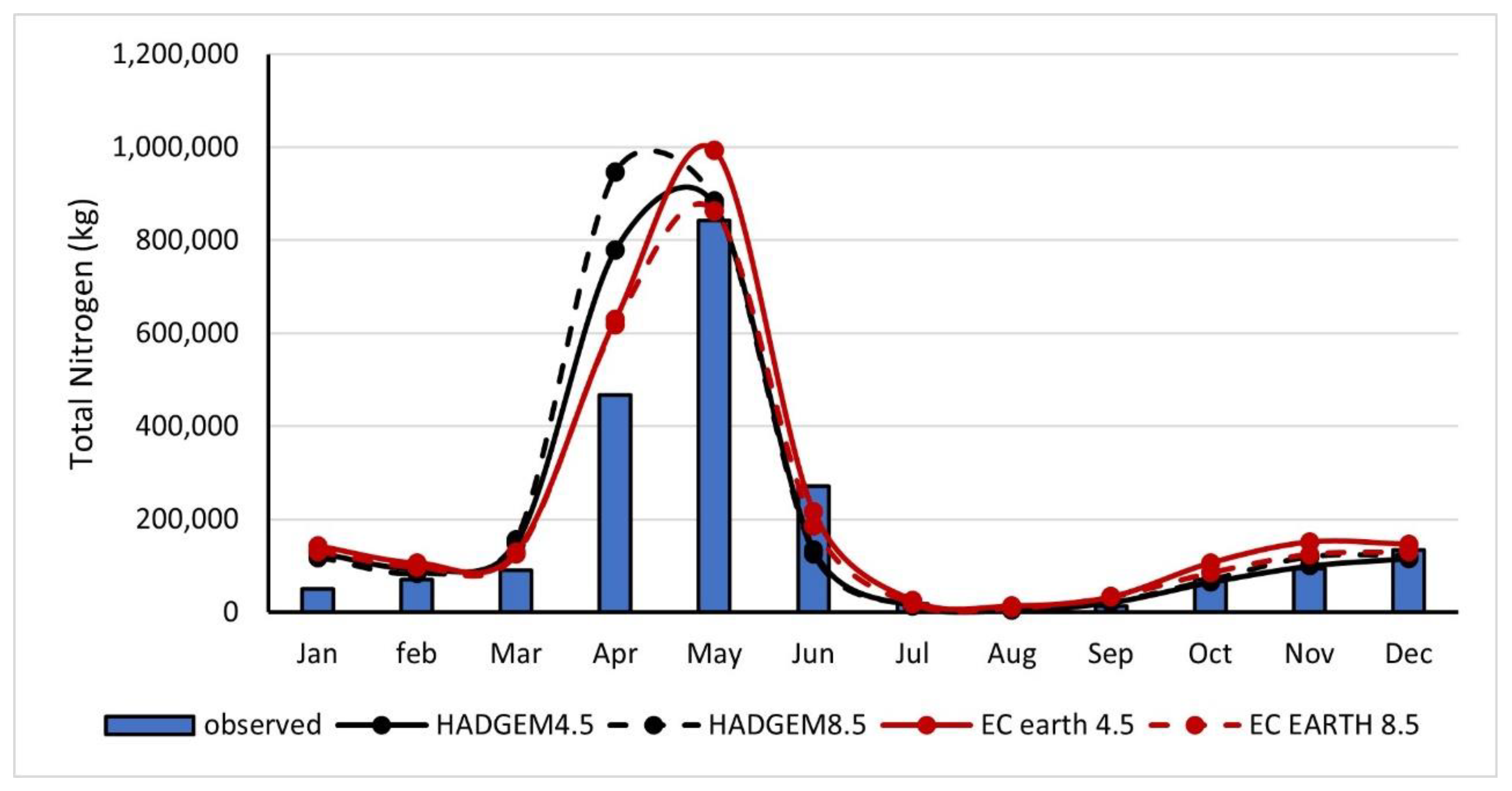
3.3.3. Climate Change Impact on TN Load

The climate change had a variable pattern of impact on average TN load from the watershed. Average TN load for the period of 2021 to 2040 increased by 9% to 38%, while the change in average TN load for 2041–2060 was decreased by 17% and increased by 10%, and that for 2061 to 2080 was decreased by 8% and increased by 10%. The summary of the percentage change in TN load during the period of 2021 to 2040, 2041 to 2060 and 2061 to 2080 for climate scenarios, RCP 4.5 and RCP 8.5 of the GCM models, HadGEM2 and EC-Earth are presented in Table 5.
Observed monthly TN load and model simulated average monthly TN load under both climate scenarios of both models was predicted highest during May and lowest during August. Monthly average TN load increased or decreased during the year based on the GCM models and their RCP climate scenarios. Monthly average TN load increased by 155% and 135% in January for the RCP 4.5 and 8.5 of the HadGEM2 model, respectively, whereas average TN load decreased by 50% and 54% in June for the RCP 4.5 and 8.5 of HadGEM2 model, respectively. Similarly, average monthly TN load increased by 184% and 161% in January for the RCP 4.5 and 8.5 of the EC-Earth model, respectively, whereas average TN load decreased by 21% and 32% in June for the RCP 4.5 and 8.5 of EC-Earth model, respectively. The average monthly TN load under climate scenarios RCP 4.5 and RCP 8.5 of the GCM models, HadGEM2 and EC-Earth are given in Figure 8.
Average monthly TN load as predicted by SWAT model based on climate change scenarios were compared with the observed monthly TN load data. Climate change data from the HadGEM2 and EC-Earth were applied to the SWAT model. The SWAT model simulated result showed peak TN load in April according to HadGEM2, whereas the EC-earth model showed peak TN load in May, similar to the observed monthly TN load. This may have been caused due to the change in surface temperature and precipitation pattern, planting/harvesting time, fertilization techniques, and increased fallow period of cultivable lands [32,33].

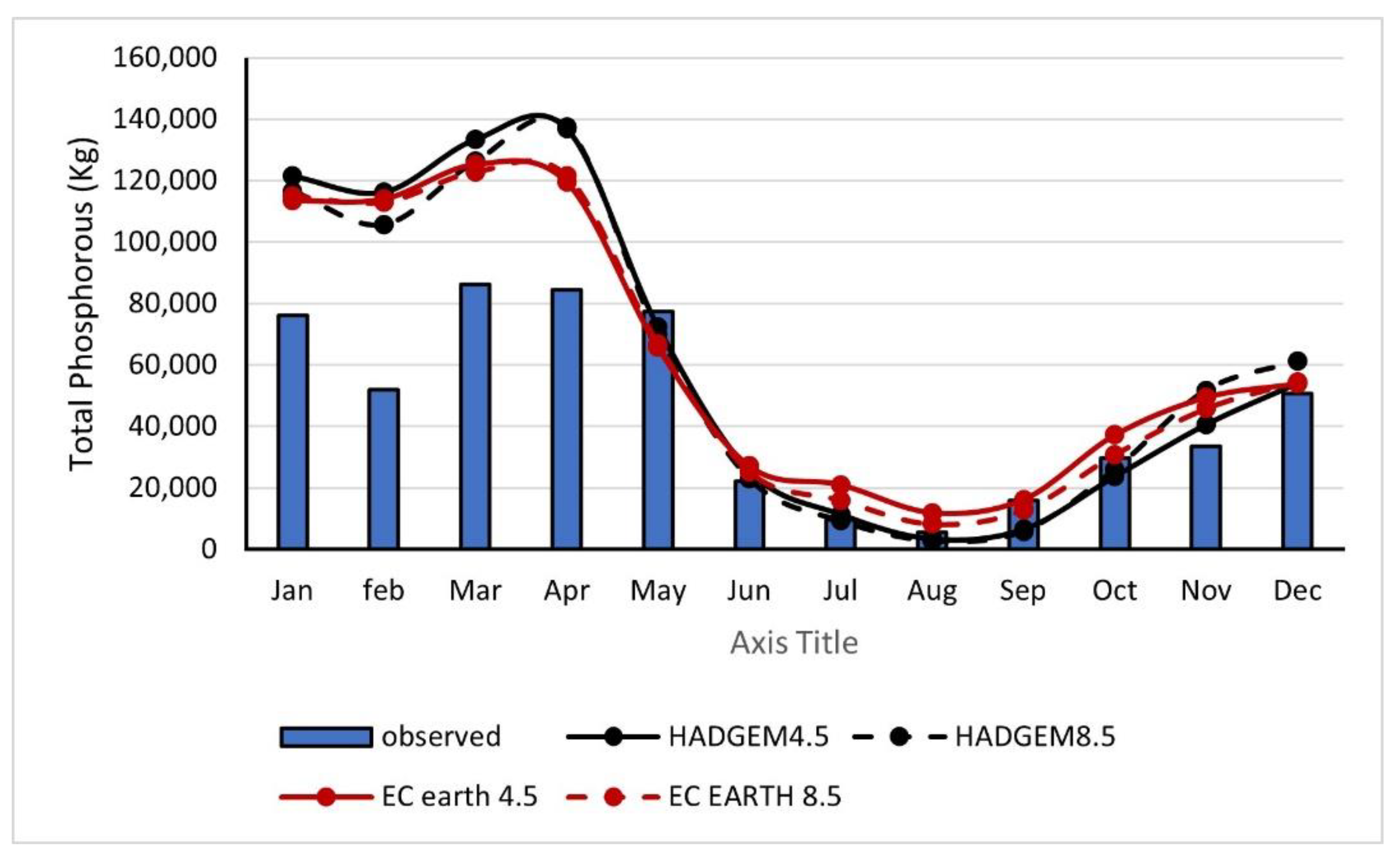
3.3.4. Climate Change Impact on Monthly TP Load

The change in monthly average TP load for the period of 2021 to 2040 was increased by 28% to 37%, while the change in average TP load for the 2041–2060 time period was decreased by 5% and increased by 9%, and that for the 2061 to 2080 time period was decreased by 1% and increased by 11%. The summary of the percentage change in TP load during the period of 2021 to 2040, 2041 to 2060 and 2061 to 2080 for climate scenarios, RCP 4.5 and RCP 8.5 of GCM models, HadGEM2 and EC-Earth are presented in Table 6.
Average monthly TP load was predicted maximum during April for both climate scenarios, RCP 4.5 and RCP 8.5, of HadGEM2 model, but the EC-Earth model climate scenarios had maximum TP load during January. Average monthly TP load was simulated lowest during August for both climate scenarios of both the models. Average TP load increased by 123% and 103% in February according to RCP 4.5 and 8.5 of the HadGEM2 model, while average TP load decreased by 58% and 63% in September according to RCP 4.5 and 8.5 of the HadGEM2 model. Similarly, average TP load increased by 123% in July and 117% in February according to RCP 4.5 and 8.5 of EC-Earth model while average TP load decreased by 15% in May and by 19% in September according to RCP 4.5 and 8.5 of EC-Earth model. Average monthly TP load under climate scenarios RCP 4.5 and RCP 8.5 of the GCM models, HadGEM2 and EC-Earth, are given in Figure 9.
Average monthly TP load as predicted by the SWAT model based on climate change scenarios were compared with the observed monthly TP load data. The greatest amount of monthly TP load was observed for March and April according to the climate change data used in the SWAT model. The greater amount of TP could have been caused by the greater amount of flow during these periods. TP is the sum of phosphorous attached to sediment particle, phosphorous attached to organic matter, soluble phosphorous, and tile phosphorous exported through subsurface drains [34].

4. Conclusions

Two RCP scenarios of two GCM models were used in the SWAT model to assess the climate change conditions and their effect on water quantity and quality during 2020–2080. The average amount of streamflow, sediment, TN, and TP load for every 20 years varied significantly under different RCP climate scenarios of two GCM models as predicted by the SWAT model. Similarly, average monthly values of streamflow, sediment, TN and TP load for 2020–2080 were observed to be significantly different than that of current monthly values. Generally, monthly average values of streamflow, TN, and TP were increased during April and May, but these values were decreased during August and September. The SWAT model simulated sediment concentrations values were slightly lower than the observed value for both the climate scenarios of both models. The SWAT simulated sediment concentration was not only dependent on streamflow but also on net precipitation and precipitation intensity, water holding capacity of soils and landcover type. Monthly average TN and TP load were predicted to be 10% to 38% greater during the climate period 2021 to 2040 than other climate periods. Monthly average TN and TP loads as predicted by the SWAT model under two RCP scenarios of two models varied from as low as 63% to as high as 184%, when compared with the observed monthly average TN and TP loads. Changes in monthly average TN and TP loads were mainly due to changes in surface temperature and precipitation pattern, alteration of planting/harvesting time, and fertilization methods. The change in hydrology and water quality was mainly attributed to the change in surface temperature, precipitation pattern and flow in the stream. Apart from that, water holding capacity of soil and landcover type also affect hydrology and water quality. The change in streamflow, sediment and nutrients are also influenced by human activities such as agricultural operation, construction, and mining [35]. The prediction of the future hydrological and water quality scenarios based on different climate scenarios input using two climate models developed in this study, will be useful in the development and implementation of effective watershed management mitigation strategies in the near and far future.

Author Contributions

Model run, data analysis and original draft preparation were done by A.R.; and development of concept, supervision, review and overall editing were done by P.B.P. All authors have read and agreed to the published version of the manuscript.

Funding

This research was funded by USDA/NIFA-AFRI grant award # 2017-67020-26375.

Data Availability Statement

Not applicable.

Acknowledgments

Authors would like to acknowledge the financial support from AFRI competitive grant award # 2017-67020-26375 from the USDA/NIFA, and Bagley College of Engineering at Mississippi State University for this project. The authors wish to thank Yazoo Mississippi Delta Joint Water Management District; United States Geological Survey (USGS); and all other collaborators for providing necessary data for this study.

Conflicts of Interest

Authors declare no conflict of interest.

References

  1. IPCC. Global Warming of 1.5 °C an IPCC Special Report on the Impacts of Global Warming of 1.5 °C above Pre-Industrial Levels and Related Global Greenhouse Gas Emission Pathways, in the Context of Strengthening the Global Response to the Threat of Climate Change, Sustainable Development, and Efforts to Eradicate Poverty; IPCC: Geneva, Switzerland, 2018. [Google Scholar]
  2. Robinson, S. Climate change adaptation in SIDS: A systematic review of the literature pre and post the IPCC Fifth Assessment Report. Wiley Interdiscip. Rev. Clim. Chang. 2020, 11, e653. [Google Scholar] [CrossRef]
  3. Lindner, M.; Maroschek, M.; Netherer, S.; Kremer, A.; Barbati, A.; Garcia-Gonzalo, J.; Seidl, R.; Delzon, S.; Corona, P.; Kolström, M. Climate change impacts, adaptive capacity, and vulnerability of European forest ecosystems. For. Ecol. Manag. 2010, 259, 698–709. [Google Scholar] [CrossRef]
  4. Li, Z.; Liu, W.-Z.; Zhang, X.-C.; Zheng, F.-L. Assessing the site-specific impacts of climate change on hydrology, soil erosion and crop yields in the Loess Plateau of China. Clim. Chang. 2011, 105, 223–242. [Google Scholar] [CrossRef]
  5. Semenov, M.A.; Brooks, R.J.; Barrow, E.M.; Richardson, C.W. Comparison of the WGEN and LARS-WG stochastic weather generators for diverse climates. Clim. Res. 1998, 10, 95–107. [Google Scholar] [CrossRef] [Green Version]
  6. Dakhlalla, A.O.; Parajuli, P.B. Sensitivity of Fecal Coliform Bacteria Transport to Climate Change in an Agricultural Watershed. J. Water Clim. Chang. 2020, 11, 1250–1262. [Google Scholar] [CrossRef]
  7. Chen, Y.; Marek, G.W.; Marek, T.H.; Moorhead, J.E.; Heflin, K.R.; Brauer, D.K.; Gowda, P.H.; Srinivasan, R. Simulating the impacts of climate change on hydrology and crop production in the Northern High Plains of Texas using an improved SWAT model. Agric. Water Manag. 2019, 221, 13–24. [Google Scholar] [CrossRef]
  8. Ouyang, Y.; Parajuli, P.B.; Feng, G.; Leininger, T.D.; Wan, Y.; Dash, P. Application of Climate Assessment Tool (CAT) to Estimate Climate Change Impacts on Water Quality for Local Watersheds. J. Hydrol. 2018, 563, 363–371. [Google Scholar] [CrossRef]
  9. Aawar, T.; Khare, D. Assessment of climate change impacts on streamflow through hydrological model using SWAT model: A case study of Afghanistan. Model. Earth Syst. Environ. 2020, 6, 1427–1437. [Google Scholar] [CrossRef]
  10. Bhatta, B.; Shrestha, S.; Shrestha, P.K.; Talchabhadel, R. Evaluation and application of a SWAT model to assess the climate change impact on the hydrology of the Himalayan River Basin. Catena 2019, 181, 104082. [Google Scholar] [CrossRef]
  11. Yu, Z.; Man, X.; Duan, L.; Cai, T. Assessments of Impacts of Climate and Forest Change on Water Resources Using SWAT Model in a Subboreal Watershed in Northern Da Hinggan Mountains. Water 2020, 12, 1565. [Google Scholar] [CrossRef]
  12. Taylor, K.E.; Stouffer, R.J.; Meehl, G.A. An overview of CMIP5 and the experiment design. Bull. Am. Meteorol. Soc. 2012, 93, 485–498. [Google Scholar] [CrossRef] [Green Version]
  13. Bekele, D.; Alamirew, T.; Kebede, A.; Zeleke, G.; Melesse, A.M. Modeling climate change impact on the Hydrology of Keleta watershed in the Awash River basin, Ethiopia. Environ. Modeling Assess. 2019, 24, 95–107. [Google Scholar] [CrossRef]
  14. Buras, A.; Menzel, A. Projecting tree species composition changes of European forests for 2061–2090 under RCP 4.5 and RCP 8.5 scenarios. Front. Plant Sci. 2019, 9, 1986. [Google Scholar] [CrossRef] [Green Version]
  15. Koo, K.A.; Kong, W.-S.; Nibbelink, N.P.; Hopkinson, C.S.; Lee, J.H. Potential effects of climate change on the distribution of cold-tolerant evergreen broadleaved woody plants in the Korean Peninsula. PLoS ONE 2015, 10, e0134043. [Google Scholar]
  16. Nilawar, A.P.; Waikar, M.L. Impacts of climate change on streamflow and sediment concentration under RCP 4.5 and 8.5: A case study in Purna river basin, India. Sci. Total. Environ. 2019, 650, 2685–2696. [Google Scholar] [CrossRef] [PubMed]
  17. Semenov, M.A.; Barrow, E.M. Use of a stochastic weather generator in the development of climate change scenarios. Clim. Chang. 1997, 35, 397–414. [Google Scholar] [CrossRef]
  18. Kim, H.K.; Parajuli, P.B.; Filip To, S.D. Assessing impacts of bioenergy crops and climate change on hydrometeorology in the Yazoo River Basin, Mississippi. Agric. For. Meteorol. 2013, 169, 61–73. [Google Scholar] [CrossRef]
  19. Semenov, M.A.; Stratonovitch, P. Use of multi-model ensembles from global climate models for assessment of climate change impacts. Clim. Res. 2010, 41, 1–14. [Google Scholar] [CrossRef] [Green Version]
  20. Parajuli, P.B.; Jayakody, P.; Sassenrath, G.F.; Ouyang, Y. Assessing the impacts of climate change and tillage practices on stream flow, crop and sediment yields from the Mississippi River Basin. Agric. Water Manag. 2016, 168, 112–124. [Google Scholar] [CrossRef] [Green Version]
  21. Parajuli, P.B.; Jayakody, P.; Sassenrath, G.F.; Ouyang, Y.; Pote, J.W. Assessing the impacts of crop-rotation and tillage on crop yields and sediment yield using a modeling approach. Agric. Water Manag. 2013, 119, 32–42. [Google Scholar] [CrossRef]
  22. Arnold, J.G.; Srinivasan, R.; Muttiah, R.S.; Williams, J.R. Large area hydrologic modeling and assessment part I: Model development 1. J. Am. Water Resour. Assoc. 1998, 34, 73–89. [Google Scholar] [CrossRef]
  23. Gassman, P.W.; Reyes, M.R.; Green, C.H.; Arnold, J.G. The soil and water assessment tool: Historical development, applications, and future research directions. Trans. ASABE 2007, 50, 1211–1250. [Google Scholar] [CrossRef] [Green Version]
  24. Neitsch, S.L.; Arnold, J.G.; Kiniry, J.R.; Williams, J.R.; King, K.W. Soil and Water Assessment Tool Theoretical Documentation, Version 2005; USDA-ARS Grassland; Soil Water Research Laboratory: Temple, TX, USA, 2005; p. 8. [Google Scholar]
  25. Licciardello, F.; Toscano, A.; Cirelli, G.L.; Consoli, S.; Barbagallo, S. Evaluation of sediment deposition in a Mediterranean reservoir: Comparison of long term bathymetric measurements and SWAT estimations. Land Degrad. Dev. 2017, 28, 566–578. [Google Scholar] [CrossRef]
  26. Tan, M.L.; Gassman, P.W.; Cracknell, A.P. Assessment of three long-term gridded climate products for hydro-climatic simulations in tropical river basins. Water 2017, 9, 229. [Google Scholar] [CrossRef] [Green Version]
  27. Risal, A.; Parajuli, P.B.; Dash, P.; Ouyang, Y.; Linhoss, A. Sensitivity of hydrology and water quality to variation in land use and land cover data. Agric. Water Manag. 2020, 241, 106366. [Google Scholar] [CrossRef]
  28. Zhang, Y.; You, Q.; Chen, C.; Ge, J. Impacts of climate change on streamflows under RCP scenarios: A case study in Xin River Basin, China. Atmos. Res. 2016, 178–179, 521–534. [Google Scholar] [CrossRef]
  29. Azim, F.; Shakir, A.S.; ur-Rehman, H.; Kanwal, A. Impact of climate change on sediment yield for Naran watershed, Pakistan. Int. J. Sediment Res. 2016, 31, 212–219. [Google Scholar] [CrossRef]
  30. Naik, P.K.; Jay, D.A. Distinguishing human and climate influences on the Columbia River: Changes in mean flow and sediment transport. J. Hydrol. 2011, 404, 259–277. [Google Scholar] [CrossRef]
  31. Zabaleta, A.; Martínez, M.; Uriarte, J.A.; Antigüedad, I. Factors controlling suspended sediment yield during runoff events in small headwater catchments of the Basque Country. CATENA 2007, 71, 179–190. [Google Scholar] [CrossRef]
  32. Olesen, J.E.; Carter, T.R.; Diaz-Ambrona, C.H.; Fronzek, S.; Heidmann, T.; Hickler, T.; Holt, T.; Minguez, M.I.; Morales, P.; Palutikof, J.P. Uncertainties in projected impacts of climate change on European agriculture and terrestrial ecosystems based on scenarios from regional climate models. Clim. Chang. 2007, 81, 123–143. [Google Scholar] [CrossRef]
  33. Olesen, J.E.; Jensen, T.; Petersen, J. Sensitivity of field-scale winter wheat production in Denmark to climate variability and climate change. Clim. Res. 2000, 15, 221–238. [Google Scholar] [CrossRef]
  34. Chaubey, I.; Migliaccio, K.W.; Green, C.H.; Arnold, J.G.; Srinivasan, R. Phosphorus modeling in soil and water assessment tool (SWAT) model. Model. Phosphorus Environ. 2006, 163–187. [Google Scholar] [CrossRef]
  35. Zhang, J.; Gao, G.; Fu, B.; Gupta, H.V. Formulating an elasticity approach to quantify the effects of climate variability and ecological restoration on sediment discharge change in the Loess Plateau, China. Water Resour. Res. 2019, 55, 9604–9622. [Google Scholar] [CrossRef]
Figure 1. Study area: Big Sunflower River Watershed in Mississippi, its sub-watersheds, river network, USGS gauges, and weather stations.
Climate 09 00165 g001
Figure 2. Comparison between observed and simulated streamflow during calibration and validation at sunflower gauge of BSRW.
Climate 09 00165 g002
Figure 3. Change in average maximum and minimum temperature for 2021 to 2040, 2041 to 2060, and 2061 to 2080 for climate scenarios RCP 4.5 and RCP 8.5 of GCM models HadGEM2 and EC-Earth.
Climate 09 00165 g003
Figure 4. Change in average daily rainfall for 2021–2040, 2041–2060 and 2061–2080 for climate scenarios, RCP 4.5, and RCP 8.5 of GCM models, HadGEM2, and EC-Earth is presented in Figure 2.
Climate 09 00165 g004
Figure 5. Average monthly maximum and minimum temperatures for climate scenarios: RCP 4.5 and RCP 8.5 of GCM models: HadGEM2 and EC-Earth along with observed monthly maximum and minimum temperature.
Climate 09 00165 g005
Figure 6. Average monthly streamflow for climate scenarios: RCP 4.5 and RCP 8.5 of GCM climate models: HadGEM2 and EC-Earth.
Climate 09 00165 g006
Figure 7. Average monthly sediment concentration for climate scenarios, RCP 4.5 and RCP 8.5 of the GCM climate models, HadGEM2 and EC-Earth.
Climate 09 00165 g007
Figure 8. Average monthly total nitrogen (TN) load for climate scenarios RCP 4.5 and RCP 8.5 of GCM climate models, HadGEM2 and EC-Earth.
Climate 09 00165 g008
Figure 9. Average monthly total phosphorous (TP) load for climate scenarios RCP 4.5 and RCP 8.5 of GCM climate models HadGEM2 and EC-Earth.
Climate 09 00165 g009
Table 1. Calibration and validation statistics for streamflow, sediment, TN and TP load at three USGS gauges of BSRW.
Streamflow Sediment yield TN TP
CalibrationValidationCalibrationValidationCalibrationValidationCalibrationValidation
R2NSER2NSER2NSER2NSER2NSER2NSER2NSER2NSE
Marigold0.680.540.660.560.750.480.590.300.590.320.450.200.850.770.670.65
Sunflower0.750.790.750.790.670.420.720.310.780.310.330.190.910.510.800.75
Leland0.750.790.880.870.590.390.660.320.800.690.480.230.810.490.670.56
Table 2. Summary of change in minimum and maximum temperature and average precipitation during 2021–2040, 2041–2060 and 2061–2080 for climate scenarios: RCP 4.5 and RCP 8.5 of GCM models: HadGEM2 and EC-Earth.
ParameterModelScenario2021–20402041–20602061–2080
Minimum TemperatureHadGEM2RCP 4.512.713.914.6
RCP 8.513.014.515.9
EC EarthRCP 4.512.412.813.2
RCP 8.512.513.214.1
Maximum TemperatureHadGEM2RCP 4.524.826.226.4
RCP 8.525.127.128.3
EC EarthRCP 4.524.324.725.1
RCP 8.524.425.126.0
PrecipitationHadGEM2RCP 4.53.93.94.3
RCP 8.54.03.63.8
EC EarthRCP 4.54.04.14.2
RCP 8.53.84.14.0
Table 3. Summary of percentage change in streamflow during 2021–2040, 2041–2060 and 2061–2080 for climate scenarios: RCP 4.5 and RCP 8.5 of GCM models: HadGEM2 and EC-Earth.
ModelScenario2021–20402041–20602061–2080
HadGEM2RCP 4.55017
RCP 8.515−1913
EC_EarthRCP 4.51923
RCP 8.5513−3
Table 4. Summary of change in sediment concentration during 2021–2040, 2041–2060 and 2061–2080 for climate scenarios: RCP 4.5 and RCP 8.5 of GCM models: HadGEM2 and EC-Earth.
ModelScenario2021–20402041–20602061–2080
HadGEM2RCP 4.5−12−27
RCP 8.5−6−147
EC_EarthRCP 4.5−3−12
RCP 8.5−104−1
Table 5. Summary of percentage change in TN load during 2021–2040, 2041–2060 and 2061–2080 for climate scenarios: RCP 4.5 and RCP 8.5 of GCM models: HadGEM2 and EC-Earth.
ModelScenario2021–20402041–20602061–2080
HadGEM2RCP 4.514−110
RCP 8.538−177
EC_EarthRCP 4.537−11−1
RCP 8.5910−8
Table 6. Summary of percentage change in TP load during 2021–2040, 2041–2060 and 2061–2080 for climate scenarios RCP 4.5 and RCP 8.5 of GCM models HadGEM2 and EC-Earth.
ModelScenario2021–20402041–20602061–2080
HadGEM2RCP 4.530311
RCP 8.537−58
EC_EarthRCP 4.53721
RCP 8.5289−1
Publisher’s Note: MDPI stays neutral with regard to jurisdictional claims in published maps and institutional affiliations.

