Assessment of Seasonal Winter Temperature Forecast Errors in the RegCM Model over Northern Vietnam

Abstract

This study verified the seasonal six-month forecasts for winter temperatures for northern Vietnam in 1998–2018 using a regional climate model (RegCM4) with the boundary conditions of the climate forecast system Version 2 (CFSv2) from the National Centers for Environmental Prediction (NCEP). First, different physical schemes (land-surface process, cumulus, and radiation parameterizations) in RegCM4 were applied to generate 12 single forecasts. Second, the simple ensemble forecasts were generated through the combinations of those different physical formulations. Three subclimate regions (R1, R2, R3) of northern Vietnam were separately tested with surface observations and a reanalysis dataset (Japanese 55-year reanalysis (JRA55)). The highest sensitivity to the mean monthly temperature forecasts was shown by the land-surface parameterizations (the biosphere−atmosphere transfer scheme (BATS) and community land model version 4.5 (CLM)). The BATS forecast groups tended to provide forecasts with lower temperatures than the actual observations, while the CLM forecast groups tended to overestimate the temperatures. The forecast errors from single forecasts could be clearly reduced with ensemble mean forecasts, but ensemble spreads were less than those root-mean-square errors (RMSEs). This indicated that the ensemble forecast was underdispersed and that the direct forecast from RegCM4 needed more postprocessing.

1. Introduction

In climate forecasting, an understanding of factors external to climate systems, such as solar activities, and improved forecasting skills for internal climate system factors, such as the teleconnections of the global atmospheric and oceanic circulations, have been played key roles in seasonal to decadal climate predictions [1,2].

The current forecasting techniques still revolve around traditional statistical methods and using numerical forecasting models, but the use of numerical models is the most preferred [1,3]. To solve the forecasting problems, numerical models require the current status of the climate system, in particular the actual climate observations, as initial conditions to initialize the model. Ocean data play an important role in this process. Advances in climate models on a global scale allow for the full description of global circulations and their interactions with initial conditions. However, the limitations of horizontal resolutions lead to fewer details in projected surface climatology. Other global aspects affected by different local features (land use, topography, water fraction, etc.) lead to difficulties in having a general physical-parameterization scheme for different climatological areas. These issues can be handled with regional climate models that can flexibly implement various physical parameterizations at higher horizontal resolutions within a limited computing domain [3,4].

Regarding seasonal forecasts, the understanding of El Niño Southern Oscillation (ENSO) teleconnection and many advanced techniques in climate modeling have improved the skill of the seasonal forecasting. For example, the climate forecast system (CFS) within the global climate data assimilation system of the National Centers for Environmental Prediction (NCEP) has made significant improvements in subseasonal (up to 4–5 weeks, e.g., major fluctuations in tropical weather, such as the Madden–Julian oscillation) to seasonal forecasting (Saha et al. in 2014 [5]) and in the detailed analysis of ENSO with its reanalysis dataset [6]. Other issues are forecast uncertainties due to the unpredictability of Earth’s dynamical components in the climate system (e.g., atmosphere and oceans) and limitations in modeling (numeric, dynamics, physics, etc.). Forecast uncertainties can be reduced with an ensemble forecast system on both global and regional scales, allowing us to define a probability range for the seasonal outlook. Advances in ensemble forecasts have produced close probabilistic predictions as tools to estimate the magnitude of uncertainties [7,8]. A typical example is the ENSO variations that highly depend on the status and variation in sea-surface temperatures predicted with CFSv2 (CFS version 2), with which a number of single forecasts are gathered and recreated into an ensemble forecast system [5]. These ensemble members include updated conditions from global analyses and uncertainty information after every run and provide a probability trend for ENSO events.

While seasonal prediction has seen significant improvements, decadal prediction is much less skillful [2]. Many approaches to improving the decadal climate prediction have been proposed, such as extracting small signals from the means of large ensembles and diagnosing their impacts on the initial condition in order to improve the prediction skill for precipitation and atmospheric circulation in addition to temperature [1] or using a forecast system that accounts for both internal variability and externally forced changes to improve surface temperature forecasts throughout a decade [9].

Due to the expansion of industrial areas and increased emissions of natural aerosols, the impact of anthropogenic forcing on century timescale projections should also be taken into account [2]. In terms of natural forcing as a result of solar and volcanic activities, dedicated and special analysis is needed to project the anomalies in the global and regional natural atmospheric patterns and oceanic variability [2].

Here, the use of a dynamical forecast system on the regional scale to provide seasonal forecasts over northern Vietnam (NVN) will be analyzed. For agricultural countries such as Vietnam, winter temperature conditions are one of the most relevant weather parameters in society. Severe winter conditions, such as the frequent occurrence of severe cold spells in northern and north–central Vietnam in the winter months (December, January and February) and subzero-temperature conditions with snow and frost, cause great damage to rice cultivation, vegetable, and fruit-tree cropping systems and livestock every year. Therefore, seasonal forecasts of winter temperatures in the 1–6 months prior facilitates the preparedness in agricultural production. This paper is divided into four main sections. Section 2 focuses on the description of the research area and its relevant works in terms of seasonal forecasting, the dataset, the model, experimental designs, and verification methods. Section 3 presents the assessment of the forecasts, and conclusions are provided in Section 4.

2. Research Area, Model, Experimental Designs, Dataset, and Verification Methods

2.1. Research Area and Relevant Studies

The great range of latitudes (from 8° N to 23° N) and elevations in Vietnam diversifies the climate of Vietnam, dividing the country into three different parts, with distinguishable climates, from north to south. On the basis of geographic conditions and local characteristics, several studies have divided the climate of Vietnam into three main climate regions: northern Vietnam (NVN) (from 20° N to 23° N), characterized by a tropical monsoon climate with four distinguishable seasons and typically high humidity; southern Vietnam (from 8° N to 12° N), characterized by a moderate tropical climate with dry and rainy seasons; and central Vietnam (from 12° N to 20° N), which is a narrow area with highly complex topography. Its climate is a combination of the northern and southern climates [10,11,12]. In this study, NVN and its winter-temperature climatology were the research areas. NVN was divided into three subclimate regions, denoted as R1, R2 and R3 (see Figure 1 for the geographic details for Vietnam and NVN).

In the winter, NVN is under the impact of the northeastern monsoon from November to April caused by planetary circulation, i.e., the East Asia winter monsoon. The northeastern monsoon is characterized by the Siberian high (denoted as SH) at the surface level with low-level northeastern winds. During the active phase of the northeastern monsoon, northeastern winds are enhanced in the sea by strong convection, and severe weather occurs in Southeast Asia and maritime continents. Various studies have found interactions between the East Asia winter monsoon and large-scale teleconnections, such as ENSO, sea surface temperature (SST) anomalies in the North Pacific, and the polar vortex [13,14]. Chen et al. in 2000 [15] also proposed cases in which unfavorable atmospheric flow patterns in East Asia during El Niño conditions may inhibit southward outbreaks of cold air, resulting in a weaker East Asia winter monsoon. Similarly, Yuan and Yang in 2012 [16] suggested an inverse connection between the East Asia winter monsoon and El Niño over the northwestern Pacific and parts of East Asia. Yu et al. in 2012 [6] found a strong relationship between the variation in sea surface temperature in the central tropical Pacific and the sea level pressure in the extratropical Pacific. With the increase in sea surface temperatures over the central tropical Pacific due to the strong Harley circulation and the small weakened Walker circulation, more frequent occurrences of ENSO event were observed in this area. By using the Met Office global seasonal and decadal prediction system (an ensemble forecast system based on the Hadley Centre Global Environmental Model to investigate the driving roles of ENSO and sudden stratospheric warming events), the recent work by Lim et. al., 2018 [17], showed a significant skill in seasonal prediction for the winter temperature variations (especially for extreme events) over the Korean Peninsula.

Another aspect regarding to the application of regional climate models is the intercontinental interaction between monsoons and El Niño/Southern Oscillation (ENSO) teleconnections, such as the ENSO−Indian monsoon, ENSO−West African monsoon, and ENSO-East Asian monsoon, which require a sufficiently wide domain to be simulated [18]. These interactions remain a challenge for regional climate modeling.

For the climatology in Vietnam, many recent studies have been carried out by using both global and regional climate models [10,11,19,20,21]. Ngo-Duc et al. in 2012 [19] attempted to assess future climate conditions in the Red River Delta region (R3 subclimate region of NVN) with regional climate model version 3 (RegCM3). The results showed that RegCM3 reproduced temperature and precipitation patterns fairly well in the baseline period but showed systematic cold biases, while future temperatures were predicted to slightly increase. Ngo-Duc et al. in 2014 [11] used three different regional climate models with three different global climate models to simulate ensemble climate prediction products for Vietnam for the period of 2000–2050. While these models showed consistency in their forecasts, and the ensemble mean was demonstrated to outperform the individual forecasts, they also showed some significant systematic biases in each individual model that led to large uncertainties. Phan-Van et al. in 2014 [20] investigated the seasonal forecast ability of RegCM (version 4.2) for Vietnam and suggested some postprocessing procedures (successive bias correction) to improve the skill of RegCM. Recent work [21] uses RegCM to study seasonal rainfall over Vietnam with CFS hindcast data to assess the predictability of these data during the past 10 years before testing the seasonal rainfall forecast for the period of 2012–2014 with CFS operational forecast data. The results showed the ability of downscaling forecasts to capture the variability of Asian monsoons and rainfall, particularly in NVN and in transitional, dry, and rainy seasons.

2.2. Model

In the present study, the regional climate model (RegCM) version 4.6.1, developed at the Abdus Salam International Centre for Theoretical Physics (ICTP), was applied (RegCM4 in this study). RegCM4 is a sigma-p vertical coordinate model with multiple physics configurations that can provide various sensitivity and localizing experiments for various global areas [4,22]. For the Vietnam area, the studies [20,21,23] used RegCM with the community climate model (CCRM) for radiation, biosphere−atmosphere transfer scheme (BATS) for the land-surface process, and Grell for cumulus parameterizations for seasonal temperature and rainfall predictions and tropical cyclone detection over the northwestern Pacific.

Currently, RegCM4 can use the modified Holtslag et al., 1990 [24], scheme or the University of Washington (UW) scheme by Bretherton and McCaa 2004 [25] as the planetary boundary layer schemes; the subgrid explicit moisture (SUBEX) resolvable precipitation scheme by Pal et al., 2000 [26]; the longwave and shortwave fluxes, and heating rates of the radiation scheme of the National Center for Atmospheric Research (NCAR) community climate model (CCRM) [27]; and the rapid radiation transfer model (RRTM) [28]; the land-surface process of the biosphere−atmosphere transfer scheme (BATS) by Dickinson et al., 1993 [29], and community land model version 4.5 (CLM) [30]; and the cumulus convection schemes by the modified Kuo [31], Grell 1993 (GR) [32], Emanuel 1991 [33], Tiedtke 1996 (TD) [34], and Kain–Fritsch 1990 [35] and 2004 (KF) [36]. All references for the physical parameterizations can be found in [4]. The model can be downloaded from the web-based project-management software SourceForge [37].

2.3. Experimental Design

In climate forecasts, apart from the importance of lateral boundary conditions from lower-resolution forecasts, the model physics plays a key role in providing the climate for different regions, and the selection of a suitable physics scheme is still a challenge. The following section reviews recent studies on selecting physical configurations for the RegCM model that is used in this study.

For example, [38] used the perturbed physics ensemble approach for RegCM (version 2) to simulate precipitation for two 60-day periods covering wet and dry extremes over the central United States. Focusing on drought and flood cases, the results showed that for flood cases, an ensemble forecast can increase the probability of detection, and, for drought cases, it can decrease the false alarm rate; the study suggested that such approaches should be studied more in regional climate modeling. The authors of [39] investigated sensitivity tests in two planetary boundary layer (PBL) parameterizations in RegCM (version 4.2) for the European domain. The results showed that a suitable PBL can help to reduce model bias, e.g., the UW scheme can reduce winter warm bias over northeastern Europe or summer warm bias over central Europe. The authors of [40] provided a sensitivity study of RegCM4 to different convective schemes over West Africa. The three schemes in this study are Emanuel, Grell, and Tiedtke, and the combinations of Emanuel and Grell over land and sea were applied for the period of November 2002–December 2004. The results suggested the use of the Emanuel convective scheme for the West African climate system.

With regard to using an ensemble approach to reduce uncertainties in modeling, perturbation methods for initial and lateral boundary conditions are commonly used in weather forecasts with a lead time of up to 10 days. With regard to climate forecasts, the very high uncertainties relating to climatology timescales (such as climate projection or change scenarios) make it difficult to generate reasonable ensemble spreads, and an enormous amount of computational resources is required when the number of ensemble sizes is large. In climate modeling, the sets of ensembles are based on two main methods, multimodel ensembles (MMEs) and perturbed physics ensembles (PPEs) [41,42]. Each method has its own advantages. MMEs are often found in intercomparison projects such as the Coupled Model Intercomparison Project (CMIP) [43] or the Prediction of Regional scenarios and Uncertainties for Defining EuropeaN Climate change risks and Effects (PRUDENCE) [44] and can therefore take advantage of the optimal results of each project for each model. However, each model has its own framework (physics, dynamics, numerics); therefore, in the combination of different models to create an ensemble system, the uncertainties or the probability distribution of the forecast of the ensemble system may not be representative, as other ensemble methods, such as the breeding method, can simulate the growing errors [42,45]. PPEs create perturbations by varying uncertain parameters of physical-parameterization schemes within a single-mode structure and are therefore able to sample a wide range of structural choices that may impact model errors, climate-change feedbacks, and climate forcing [42]. In PPEs, coming with perturbation-parameter processes, e.g., varying the master turbulent length scale in PBL schemes in [39], the changeable physical schemes in each model can also be used to minimize the computing cost while still generating ensemble members with different physics within a dynamical framework. For example, in the Southeast Asia regional climate downscaling/coordinated regional climate downscaling experiment—Southeast Asia (SEACLID/CORDEX—SEA) project, [46] evaluated the simulation of extreme rainfall and temperature indices by using 18 experiments with different combinations of cumulus parameterization and ocean flux schemes in RegCM4. This approach can be referred to as the multiphysics ensemble approach.

Within this study, on the basis of RegCM4, different physics configurations (land-surface process, cumulus, and radiation parameterizations) in RegCM were first alternated to generate single forecasts. We used two radiation schemes, CCRM and RRTM; two land-surface processes, BATS and CLM45; and three cumulus parameterizations, Grell, Tiedtke, and Kain–Fritsch; to generate 12 different configurations.

Second, the simple ensemble forecasts were established by the combinations of those different physical runnings. We ran the basic ensemble forecast (denoted as ENS12) with 12 different configurations of RegCM4 every five days starting on the first day of the month; therefore, we performed at least six basic ensemble runs per month. The final ensemble forecasts (denoted as ENS36), with 36 members, were generated by combining three successive basic ensemble forecasts: the first final ensemble forecast was combined from the first three runs, and the second ensemble forecast was combined from the last three runs. In this study, the forecasting started in July, August, September, and October for the period of 1998–2018. For each month, there were 6 RegCM4 forecast runs. Due to the available retrospective dataset of CFSv2, some months only had 5 runs.

For the other model configurations, the horizontal resolution was set to 32 km × 32 km with 18 vertical levels. The domain forecast is shown in Figure 1a with the center at 20° N, 110° E, and the computing domain consisted of 138 × 138 grid points in the x, y dimensions. All information for experiments is listed in

Table 1. Experimental information.

Abbreviation	Model Physic Configurations
	Land Surface Scheme	Radiation Scheme	Cumulus Scheme
BAT01	BATS	RRTM	Grell
BAT02	BATS	CCRM	Grell
BAT03	BATS	RRTM	Tiedtke
BAT04	BATS	CCRM	Tiedtke
BAT05	BATS	RRTM	Kain-Fritsch
BAT06	BATS	CCRM	Kain-Fritsch
CLM01	CLM45	RRTM	Grell
CLM02	CLM45	CCRM	Grell
CLM03	CLM45	RRTM	Tiedtke
CLM04	CLM45	CCRM	Tiedtke
CLM05	CLM45	RRTM	Kain-Fritsch
CLM06	CLM45	CCRM	Kain-Fritsch

.

2.4. Dataset

2.4.1. Initial and Lateral Boundary Conditions

In this study, the NCEP CFSv2 was used for the initial and lateral boundary conditions. CFSv2, a coupled ocean–land–atmosphere dynamical seasonal prediction system, has two types of data, retrospective and operational forecasts, and has been in operation since 2004 [5,47]. The operational forecast CFSv2 has four forecasting cycles at 00:00, 06:00, 12:00, and 18:00 UTC, and each cycle has different configurations with three different types of forecasts, including forecasts of up to 9 months and seasonal and subseasonal forecasts. The retrospective CFSv2 was used for the period 1998-2011, and the operational CFSv2 was used for the period 2011–2018. CFSv2 reforecast and operational forecast data were downloaded via internet links [48,49], and only forecast data at 00 UTC were used in this study. The SST fields from CFSv2 were also used for RegCM4.

2.4.2. Observational Data

The number of observational stations in Vietnam increased from 89 in 1988 to 186 in 2017, with 4 or 8 observations per day, and approximately 24–28 stations have been reported to the World Meteorological Organization (WMO). The highest station density is in the R3 region, with approximately 1 station per 25 km² area. On average, the current surface observational network density of NVN is approximately 1 station per 30 km², which is suitable for the verification of model grids with horizontal resolutions of approximately 30 km × 30 km [50]. In this study, 89 surface synoptic observation stations were used to validate the forecast of RegCM4. The distribution of stations is displayed in Figure 1b.

2.4.3. Reanalysis Data

In this study, the Japanese 55-year reanalysis (JRA55) was used to additionally validate the atmospheric circulations. JRA55 is a dataset from 1958 with many advanced techniques for numerical weather predictions (data assimilation), and it makes use of almost all available types of observations (from conventional surface- and upper-level observations to nonconventional observations, such as satellites); therefore, it can help to reanalyse global climate features and their variability [51]. The monthly JRA55 data were downloaded via Internet links [52].

2.5. Verification Methods

In this study, the forecast from RegCM4 was interpolated to station positions, and temperature was adjusted with a lapse rate of 6.5 °C/km due to the difference in the model grid and station height. The average daily temperature was calculated from four observation times, 00:00, 06:00, 12:00, and 18:00 UTC, and the monthly temperature was the average of the daily temperatures in a given month. The area average (for R1, R2, and R3) was the mean value from all stations in this area. Verifications were carried out for the winter months, December, January, and February, for a forecast time of up to 6 months.

The validation scores include the mean error (ME), mean absolute error (MAE), root-mean-square error (RMSE) and correlation coefficients [53]. The climatology forecast (CLIM) for a given year is equal to the mean of 10-15-year observations before this year. The ensemble means were calculated as the average of all single forecasts or ensemble members. The ensemble spreads were calculated as the standard deviations of all forecast members from their ensemble means. The closer the ensemble spread was to the RMSE of the ensemble mean, the better the ensemble forecast was [54].

3. Results

3.1. Single-Forecast Performances

The general forecast performance of RegCM4 with different configurations is shown in Figure 2 for the average monthly temperature of each subclimate region via box plots, which cover 90% of all cases between hinges. Forecasts from CFS and observations are also displayed in this figure. The temperature of the R1 and R2 regions at all forecast ranges (four, five, and six months) was underestimated by the CFS forecast. Only for the R3 region was the forecast for January and February approximately equal to the observation distribution, especially at the five- and six-month forecast ranges. In general, distributions of the 12 single forecasts were closer to the observations than the CFS was for R1 and R2. The BATS forecast group clearly reduced the negative bias of CFS for R1 and R2. For R3, CFS provided a better ranges of forecast values than RegCM4.

From the 12 single forecasts, we found that the performance of the different physical configurations of RegCM4 was mostly sensitive to land-surface parameterization schemes rather than to radiation or cumulus schemes. For the R1 region, the CLM forecast distribution was closer to observations than BATS in all winter months, while BATS, similar to CFS, tended to provide lower forecast values. For the two remaining areas, R2 and R3, CLM forecasts tended to have a warmer forecast than the BATS forecasts. For the January and February forecasts, BATS forecasts were more consistent with observations than the CLM configuration. The difference between the forecast lead time was clearest in December for both BATS and CLM, especially in the R2 and R3 regions.

For the December forecast, many stations were found to have lower temperatures than those observed in the BATS configuration. At mountainous stations, the differences could reach up to 3–5 °C due to the large differences in the height of the model grids and stations. The behavior of BATS and CLM in the R3 region, a flat coastal area, was considerably different, resulting in a large ensemble spread in the ENS12 and ENS36 systems (overdispersion). A further illustration of the bias trends of BATS and CLM can be found in the ME distribution at each station, illustrating the six-month forecast range in Figure 3 for the forecast of the BAT01 and CLM01 experiments.

In terms of forecast errors, the RMSE of the BATS forecast was approximately 3.5–4.5 °C for R1, and 2.5–3.5 °C for R2 and R3, whereas this figure for the CLM forecast was approximately 2.5–3 °C for R1 and R2, and approximately 3–4 °C for R3 (

Table 2. Root-mean-square errors (RMSEs) in 1998–2018 for December, January, and February from CFS, ENS12, ENS36, and single forecasts for different subclimate regions at the four-month forecast range. The unit in °C.

Subclimate Region	R1			R2			R3
Forecast Month	Dec.	Jan.	Feb.	Dec.	Jan.	Feb.	Dec.	Jan.	Feb.
CLIM	2.26	2.19	2.45	2.32	2.41	2.53	2.44	2.87	2.64
CFS	4.61	4.19	2.51	3.93	3.92	2.08	3.76	4.13	3.05
ENS12	3.65	2.54	2.13	2.68	2.17	1.69	2.84	2.96	3.17
ENS36	3.61	2.46	2.01	2.51	2	1.44	2.39	2.58	2.76
BAT01	4.19	3.11	3.05	3.41	2.72	2.21	3.14	2.91	2.7
BAT02	4.59	3.37	3.32	3.56	2.78	2.22	2.91	2.75	2.62
BAT03	4.09	3.06	2.98	3.39	2.71	2.19	3.14	2.89	2.69
BAT04	4.74	3.53	3.56	3.6	2.77	2.19	3.08	2.87	2.79
BAT05	4.51	3.4	3.52	3.49	2.74	2.19	3.22	2.93	2.73
BAT06	5.25	3.89	4.16	3.6	2.77	2.32	2.84	2.76	2.79
CLM01	3.01	2.59	2.32	2.3	2.52	2.67	2.81	3.51	4.11
CLM02	2.57	2.61	2.5	2.15	2.53	2.7	2.86	3.36	3.84
CLM03	3.05	2.63	2.33	2.2	2.56	2.74	3.04	3.73	4.3
CLM04	2.68	2.6	2.38	2.08	2.56	2.76	3.02	3.54	4.01
CLM05	3.66	2.63	2.19	2.22	2.49	2.66	3.05	3.77	4.43
CLM06	3.06	2.45	2.14	2.06	2.48	2.64	2.85	3.32	3.92

). For the correlation information (

Table 3. Correlation coefficients for the mean monthly temperature (for December, January, and February) between the RegCM4 predictions and observations in 1998–2018 from CFS, ENS12, ENS36, and single forecasts for different subclimate regions at the four-month forecast range.

Subclimate Region	R1			R2			R3
Forecast Month	Dec.	Jan.	Feb.	Dec.	Jan.	Feb.	Dec.	Jan.	Feb.
CFS	0.21	0.29	0.01	0.33	0.38	0.07	0.08	0.32	−0.15
ENS12	0.72	0.81	0.54	0.65	0.69	0.44	0.22	0.42	−0.17
ENS36	0.75	0.85	0.62	0.68	0.72	0.52	0.25	0.51	−0.29
BAT01	0.71	0.79	0.55	0.61	0.66	0.4	0.14	0.39	−0.22
BAT02	0.69	0.79	0.57	0.6	0.65	0.43	0.15	0.37	−0.2
BAT03	0.7	0.8	0.55	0.61	0.67	0.41	0.14	0.43	−0.2
BAT04	0.69	0.79	0.51	0.6	0.66	0.4	0.17	0.42	−0.24
BAT05	0.71	0.8	0.52	0.61	0.67	0.39	0.21	0.49	−0.24
BAT06	0.7	0.8	0.55	0.6	0.67	0.43	0.2	0.41	−0.19
CLM01	0.7	0.78	0.55	0.65	0.67	0.47	0.17	0.29	−0.07
CLM02	0.72	0.79	0.54	0.66	0.67	0.44	0.21	0.29	−0.13
CLM03	0.69	0.79	0.51	0.64	0.68	0.43	0.19	0.35	−0.15
CLM04	0.72	0.79	0.5	0.65	0.68	0.43	0.22	0.35	−0.16
CLM05	0.69	0.8	0.52	0.64	0.69	0.45	0.23	0.37	−0.09
CLM06	0.72	0.81	0.55	0.66	0.69	0.48	0.23	0.32	−0.08

), RegCM4 provides a good correlation (~0.5–0.7) for the R1 and R2 regions and a quite low correlation for R3 (0.1–0.2).

The further assessment of the BATS forecast when changing radiation- or cumulus-parameterization schemes showed that, in R1 and R2 for the target months of December and January, the RRTM scheme provided better results than the CCRM scheme, with a reduction of 10%–20% in RSME. The sensitivity in February and for R3 was lower. BATS with the KF scheme showed a higher error than with the GR and TD schemes (RMSE increased by 5%–10%). For CLM, the sensitivities of the different radiation schemes were not as large or clear as those with BATS. However, the combination with CCRM had a tendency for lower error than that with RRTM.

In addition to the direct effects on surface climatology of the land-surface process schemes, a different physical configuration can have a large impact on atmospheric circulations, thereby being a main source of error. As mentioned in Section 2.1, among the various atmospheric circulation systems, the main system affecting winter weather in Vietnam is the semipermanent high-pressure Siberian system. In December or January, incursions of cold-air masses from the north or the northward extension of SH play a major role in determining the winter cold-temperature conditions in NVN. In February, SH tends to shift toward the east; therefore, cold-air masses from the north normally pass the Tonkin Gulf (centered at 20° N, 108° E) before affecting NVN and cause higher humidity and warmer conditions compared to the conditions in December and January. Figure 4 shows the situation in which the BATS forecast group (only the BAT01 forecast is shown) simulated a significant cold incursion of northern air masses for December in 2017 at the six-month forecast range. With the JRA55 reanalysis, NVN temperature was approximately 12–18 °C, and the pressure mean sea level (PMSL) contour at level 1020 hPa was approximately 20° N over NVN. Extreme cold was forecasted over the mountainous areas in the west of NVN. Over the R1 region, the observed temperature was approximately 15–16 °C, while it was underestimated by the BATS scheme at approximately 12–13 °C with a cold bias of 2–3 °C. The PMSL contour at a level of 1020 hPa reached approximately 17.5° N–18° N over NVN. With the CLM scheme (only the CLM01 forecast is shown), the forecast temperature was 0.5–1 °C higher than that of the observation at approximately 14–15 °C, with the PMSL contour at a level of 1020 hPa reaching approximately 20° N over NVN.

3.2. Ensemble Performances

The assessment of the different physical configurations shows uncertainties in the forecasts, especially with the two different land-surface processes, thereby facilitating the generation of confidence intervals for the forecast with RegCM4 for winter temperatures over NVN in a seasonal forecast range.

In Figure 2, as an example for the December forecast, the ensemble means of ENS12 and ENS36 were plotted together with the single forecasts. For subclimate region R1, in December, both ENS12 and ENS36 failed to improve the forecast due to the large negative-bias forecast from the BATS configurations. However, for the January and February forecasts, the ensemble mean forecasts were clearly matched to observation variations. In the ensemble mean forecasts, there were still many extreme colder forecast values compared to those in the observations. The RMSEs (Table 2) for R1 in January and February were approximately 2–3 °C and were lower than those of the single forecasts. The RMSE of ENS36 was 5%–10% lower than that of ENS12. For R2 and R3, the RMSEs were clearly improved, by approximately 2–2.5 °C for ENS12, and the RMSE of ENS36 was approximately 20% lower than of ENS12. The ME distributions for ENS12 in Figure 5 show the better performance of ENS12 compared with the single forecasts (Figure 3).

The improvement in ENS36 compared to ENS12 can further be seen in the MAE chart in Figure 6. In addition, the confidence intervals were also improved in ENS36 compared to ENS12, which shows that taking advantage of consecutive runs is also an effective way of minimizing errors caused by inappropriate model physics.

The evaluation of errors by forecast ranges showed that the forecast error (RMSE) for December at five and six months increased by approximately 5%–10% compared to that of a forecast term of four months (Table 2). For January and February, the forecast errors at five- and six-month forecast ranges are quite similar.

The forecast errors for R3 for February, were much higher than those for December and January due to the large positive bias of the CLM configuration groups. Additional analyses with the JRA55 dataset show that the main atmospheric circulations of CLM groups tend to forecast rapid eastward shifts in SH, enabling cold air mass advection to pass over the Tonkin Gulf before affecting NVN with more humid and warmer air than that in the actual conditions.

As mentioned in the research of Phan-Van et al., 2014 [20], the direct forecasts of RegCM for temperature in terms of seasonal forecasts for the Vietnam area was still very low skill when compared to those of CLIM. As shown in Table 2, the RMSEs of CLIM are approximately 2.2–2.5 °C, and the RMSEs for all single forecasts are approximately 2.5–4.0 °C; however, due to the a good correlation, especially for the R1 and R2 regions, further postprocessing (bias correction) was needed. The average RMSEs of ENS36 for R2 and R3 were approximately 1.5–2.2 °C for December and January, showing the improvement resulting from simply using a number of single forecasts to recreate an ensemble forecast system.

Another aspect of ensemble forecast evaluation is the ensemble spread given in Figure 7, which shows both the RMSEs and the spreads of ENS12 and ENS36. The main causes of the large differences in spread and RMSE are the large biases of the BATS (cold bias) and CLM (warm bias) forecast groups. The largest difference (~2 °C) of the spread and RMSEs was for R1 in December, and the use of difference runs as in ENS36 could provide better spread information. Although most ENS36 predictions had larger spreads than ENS12, in the case of the February forecast for the R2 region and the January forecast for the R3 region, ENS12 showed much higher consistency; in other words, if there were sudden changes in temperature during winter, combining different runs (as in ENS36) can sometimes reduce the quality of the forecasts. Overall, however, even with the improvement for the R1 and R2 regions via ensemble mean errors, the spreads were less than the RMSE, indicating the underdispersal or overconfidence of both ENS12 and ENS36. This means that the forecasts in each group of land surface process schemes (BATS or CLM) were not truly separated enough to reduce overconfidence in ENS12 and ENS36.

4. Conclusions

This paper presented the characteristics of temperature forecast errors from the RegCM4 model with different physical configurations, with a focus on a four-, five-, and six-month forecast ranges, over northern Vietnam in winter 1998–2018. The main results were as follows:

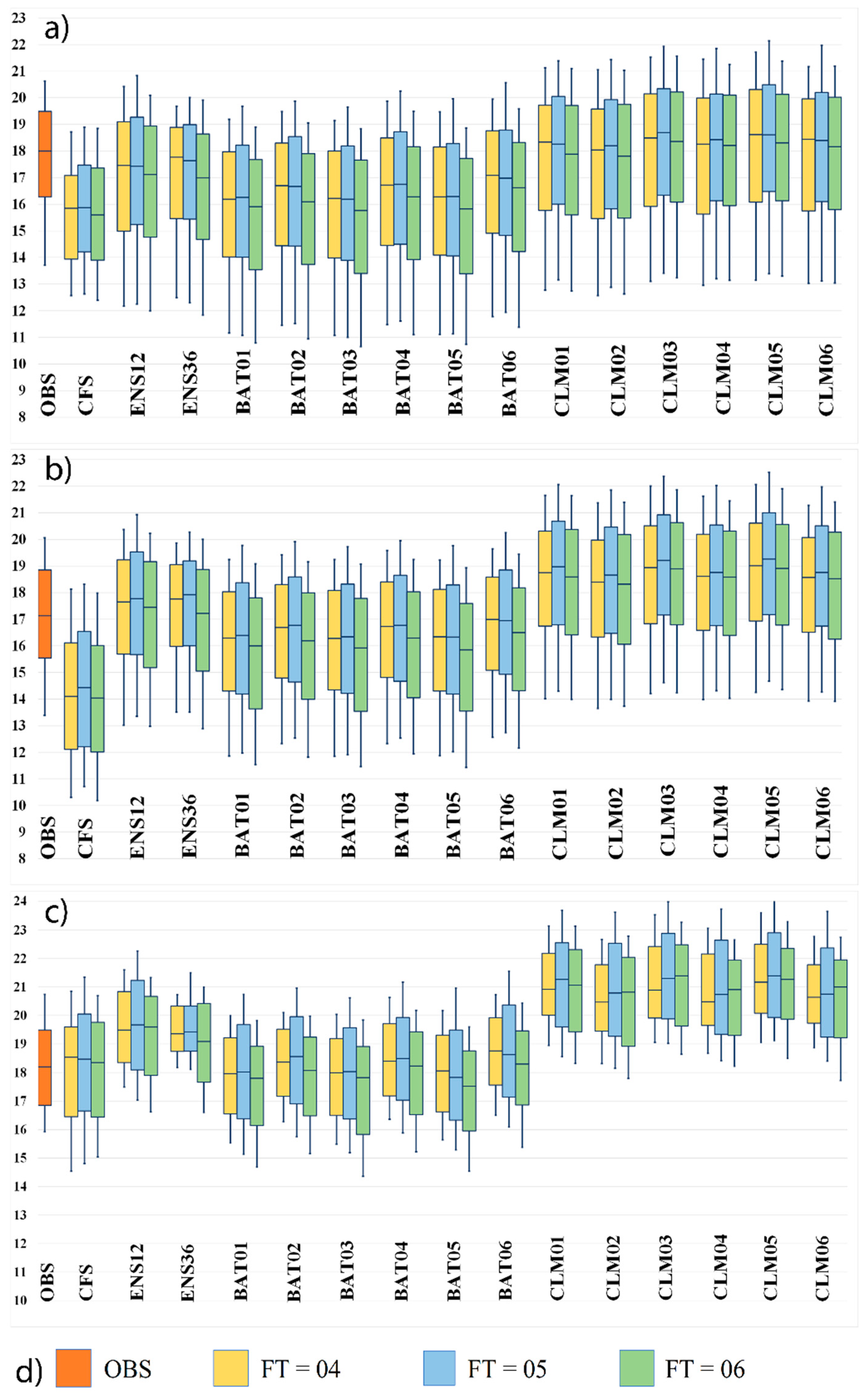
• Compared to the CFSv2 forecast, the BATS forecast group clearly reduced the negative bias of CFSv2 for the R1 and R2 regions, but CFSv2 provided better ranges of forecast values to RegCM4 for the R3 region;
• The highest sensitivity of the temperature forecast was found for land-surface parameterizations (BATS and CLM schemes), and the BATS forecast group tended to provide a lower temperature forecast than the actual observations. The CLM forecast group, on the other hand, tended to forecast higher temperatures, especially for subclimate region R3; and
• Forecast errors from single forecasts could clearly be reduced using ensemble mean forecasts, but the ensemble spreads were smaller than those RMSEs, which indicated the underdispersal of the ensemble forecast and the need for more postprocessing of the direct forecast from RegCM4.

The purpose of investing different physical schemes for RegCM4 is to find a suitable forecast not only for a given subclimate region but also for different periods of winter; therefore, using different physical schemes can help in the selection of ensemble members for ensemble forecasting. In addition to testing the typical parameters of the current physical parameterization schemes for RegCM4, more sensitivity tests with perturbed physics ensembles in seasonal winter temperature forecasts are needed to help reduce the overconfidence of the forecasts from the BATS and CLM groups.

Further studies must address the need for postprocessing to remove the large bias in single forecasts in different subclimate regions, and thereby reduce ensemble forecast overconfidence as well as the verification of climatological forecasts that require a longer sample period for hindcast/retrospective forecasts.

References

1. Smith, D.M.; Scaife, A.A.; Kirtman, B.P. What is the current state of scientific knowledge with regard to seasonal and decadal forecasting? Environ. Res. Lett. 2012, 7, 015602. [Google Scholar] [CrossRef]
2. Kushnir, Y.; Scaife, A.A.; Arritt, R.; Balsamo, G.; Boer, G.; Doblas-Reyes, F.; Matei, D. Towards operational predictions of the near-term climate. Nat. Clim. Chang. 2019, 9, 94–101. [Google Scholar] [CrossRef]
3. Fink, A.; Langhans, W.; Fosser, G.; Ferrone, A.; Ban, N.; Goergen, K.; Keller, M.; Tölle, M.; Gutjahr, O.; Feser, F.; et al. A review on regional convection-permitting climate modeling: Demonstrations, prospects, and challenges. Rev. Geophys. 2015, 53, 323–361. [Google Scholar] [CrossRef] [Green Version]
4. Gao, X.; Giorgi, F. Use of the Reg CM system over East Asia: Review and perspectives. Engineering 2017, 3, 766–772. [Google Scholar] [CrossRef]
5. Saha, S.; Moorthi, S.; Wu, X.; Wang, J.; Nadiga, S.; Tripp, P.; Behringer, D.; Hou, Y.T.; Chuang, H.Y.; Iredell, M.; et al. The NCEP climate forecast system version 2. J. Clim. 2014, 27, 2185–2208. [Google Scholar] [CrossRef]
6. Yu, J.-Y.; Lu, M.-M.; Kim, S. A change in the relationship between tropical central Pacific SST variability and the extratropical atmosphere around 1990. Environ. Res. Lett. 2012, 7, 034025. [Google Scholar] [CrossRef]
7. Min, S.-K.; Simonis, D.; Hense, A. Probabilistic climate change predictions applying Bayesian Model Averaging. Philos. Trans. R. Soc. A 2007, 365, 2103–2116. [Google Scholar] [CrossRef]
8. Tebaldi, C.; Knutti, R. The use of the multi-model ensemble in probabilistic climate projections. Philos. Trans. R. Soc. A 2007, 365, 2053–2075. [Google Scholar] [CrossRef]
9. Smith, D.; Cusack, S.; Colman, A.; Folland, C.; Harris, G.; Murphy, J. Improved Surface Temperature Prediction for the Coming Decade from a Global Climate Model. Science 2007, 317, 796–799. [Google Scholar] [CrossRef] [Green Version]
10. Ho, T.; Phan, V.; Le, N.; Nguyen, Q. Extreme climatic events over Vietnam from observational data and RegCM3 projections. Clim. Res. 2011, 49, 87–100. [Google Scholar] [CrossRef] [Green Version]
11. Ngo-Duc, T.; Kieu, C.; Thatcher, M.; Nguyen-Le, D.; Phan-Van, T. Climate projections for Vietnam based on regional climate models. Clim. Res. 2014, 60, 199–213. [Google Scholar] [CrossRef] [Green Version]
12. Phan-Van, T.; Ngo-Duc, T.; Ho, T.-M.-H. Seasonal and interannual variations of surface climate elements over Vietnam. Clim. Res. 2009, 40, 49–60. [Google Scholar] [CrossRef] [Green Version]
13. Chang, C.P.; Lu, M.M.; Wang, S. The East Asian winter monsoon. In The Global Monsoon System, 2nd ed.; World Scientific Publishing Co Pte Ltd.: Singapore, 2011. [Google Scholar]
14. Wang, L.; Lu, M.-M. The East Asian winter monsoon. In The Global Monsoon System, 3rd ed.; World Scientific Publishing Co Pte Ltd.: Singapore, 2017. [Google Scholar]
15. Chen, S.; Song, L. Recent strengthened impact of the winter arctic oscillation on the Southeast Asian surface air temperature variation. Atmosphere 2019, 10, 164. [Google Scholar] [CrossRef] [Green Version]
16. Yuan, Y.; Yang, S. Impacts of different types of El Niño on the East Asian climate: Focus on ENSO cycles. J. Clim. 2012, 25, 7702–7722. [Google Scholar] [CrossRef]
17. Lim, J.; Dunstone, N.; Scaife, A.; Smith, D. Skilful seasonal prediction of Korean winter temperature. Atmos. Sci. Lett. 2019, 1. [Google Scholar] [CrossRef]
18. Coppola, E.; Giorgi, F.; Mariotti, L.; Bi, X. RegT-Banda tropical band version of RegCM4. Clim. Res. 2012, 52, 115–133. [Google Scholar] [CrossRef] [Green Version]
19. Ngo-Duc, T.; Quang, T.N.; Trinh, L.T.; Vu, T.H.; Phan-Van, T.; Cu, P.V. Near future climate projections over the red river delta of vietnam using the regional climate model version 3. Sains Malays. 2012, 41, 1325–1334. [Google Scholar]
20. Phan-Van, T.; Van Nguyen, H.; Trinh Tuan, L.; Nguyen Quang, T.; Ngo-Duc, T.; Laux, P.; Xuan, T.N. Seasonal prediction of surface air temperature across Vietnam using the regional climate model version 4.2 (RegCM4.2). Adv. Meteorol. 2014, 2014, 245104. [Google Scholar] [CrossRef]
21. Phan-Van, T.; Nguyen-Xuan, T.; Nguyen, H.V.; Laux, P.; Pham-Thanh, H.; Ngo-Duc, T. Evaluation of the NCEP climate forecast system and its downscaling for seasonal rainfall prediction over Vietnam. Weather Forecast. 2018, 33, 615–640. [Google Scholar] [CrossRef]
22. Giorgi, F.; Coppola, E.; Solmon, F.; Mariotti, L.; Sylla, M.B.; Bi, X.; Elguindi, N.; Diro, G.T.; Nair, V.; Giuliani, G.; et al. RegCM4: Model description and preliminary tests over multiple CORDEX domains. Clim. Res. 2012, 52, 7–29. [Google Scholar] [CrossRef] [Green Version]
23. Phan-Van, T.; Trinh-Tuan, L.; Bui-Hoang, H.; Kieu, C. Seasonal forecasting of tropical cyclone activity in the coastal region of Vietnam using RegCM4.2. Clim. Res. 2015, 62, 115–129. [Google Scholar] [CrossRef] [Green Version]
24. Holtslag, A.A.M.; De Bruijn, E.I.F.; Pan, H.-L. A high resolution air mass transformation model for short-range weather forecasting. Mon. Weather Rev. 1990, 118, 1561–1575. [Google Scholar] [CrossRef]
25. McCaa, J.R.; Bretherton, C.S. A New Parameterization for Shallow Cumulus Convection and Its Application to Marine Sub-tropical Cloud-Topped Boundary Layers. Part II: Regional Sim-ulations of Marine Boundary Layer Clouds. Mon. Wea. Rev. 2004, 132, 883–896. [Google Scholar] [CrossRef]
26. Pal, J.S.; Small, E.E.; Eltahir, E.A.B. Simulation of regional—Scale water and energy budgets: Representation of subgrid cloud and precipitation processes within RegCM. J. Geophys. Res. 2000, 105, 29579–29594. [Google Scholar] [CrossRef]
27. Kiehl, J.T.; Hack, J.J.; Bonan, G.B.; Boville, B.A.; Breigleb, B.P.; Williamson, D.; Rasch, P. Description of the ncar community climate model (ccm3) (No. NCAR/TN-420+STR). Univ. Corp. Atmos. Res. 1996. [Google Scholar] [CrossRef]
28. Mlawer, E.J.; Taubman, S.J.; Brown, P.D.; Iacono, M.J.; Clough, S.A. Radiative transfer for inhomogeneous atmospheres: RRTM, a validated correlated-k model for the longwave. J. Geophys. Res. 1997, 102, 16663–16682. [Google Scholar] [CrossRef] [Green Version]
29. Dickinson, R.E.; Henderson-Sellers, A.; Kennedy, P.J. Biosphere-atmosphere transfer scheme (BATS) version 1e as coupled to the NCAR community climate model (No. NCAR/TN-387+STR). Univ. Corp. Atmos. Res. 1993. [Google Scholar] [CrossRef]
30. Brunke, M.A.; Broxton, P.; Pelletier, J.; Gochis, D.; Hazenberg, P.; Lawrence, D.M.; Leung, L.R.; Niu, G.; Troch, P.A.; Zeng, X. Implementing and Evaluating Variable Soil Thickness in the Community Land Model, Version 4.5 (CLM4.5). J. Clim. 2016, 29, 3441–3461. [Google Scholar] [CrossRef]
31. Anthes, R.A.; Hsie, E.-Y.; Kuo, Y.-H. Description of the Penn State/NCAR Mesoscale Model Version 4 (MM4); National Center for Atmosphere Research: Boulder, CO, USA, 1987.
32. Grell, G.A. Prognostic Evaluation of Assumptions Used by Cumulus Parameterizations. Mon. Weather Rev. 1993, 121, 764–787. [Google Scholar] [CrossRef] [Green Version]
33. Emanuel, K.A. A Scheme for Representing Cumulus Convection in Large-Scale Models. J. Atmos. Sci. 1991, 48, 2313–2329. [Google Scholar] [CrossRef]
34. Tiedtke, M. A Comprehensive Mass Flux Scheme for Cumulus Parameterization in Large-scale Models. Mon. Weather Rev. 1989, 117, 1779–1800. [Google Scholar] [CrossRef] [Green Version]
35. Kain, J.S.; Fritsch, J.M. A one-dimensional entraining/detraining plume model and its application in convective parameterization. J. Atmos. Sci. 1990, 47, 2784–2802. [Google Scholar] [CrossRef] [Green Version]
36. Kain, J.S. The Kain–Fritsch Convective Parameterization: An Update. J. Appl. Meteor. 2004, 43, 170–181. [Google Scholar] [CrossRef] [Green Version]
37. RegCM4 Model Source Code. Available online: https://gforge.ictp.it/gf/project/regcm (accessed on 12 April 2020).
38. Yang, Z.; Arritt, R.W. Tests of a perturbed physics ensemble approach for regional climate modeling. J. Clim. 2002, 15, 2881–2896. [Google Scholar] [CrossRef]
39. Güttler, I.; Branković, Č.; O’Brien, T.A.; Coppola, E.; Grisogono, B.; Giorgi, F. Sensitivity of the regional climate model RegCM4.2 to planetary boundary layer parameterization. Clim. Dyn. 2014, 43, 1753–1772. [Google Scholar] [CrossRef]
40. Koné, B.; Diedhiou, A.; N’datchoh, E.T.; Sylla, M.B.; Giorgi, F.; Anquetin, S.; Bamba, A.; Diawara, A.; Kobea, A.T. Sensitivity study of the regional climate model RegCM4 to different convective schemes over West Africa. Earth Syst. Dyn. 2018, 9, 1261–1278. [Google Scholar] [CrossRef] [Green Version]
41. Bellprat, O.; Kotlarski, S.; Lüthi, D.; Schär, C. Exploring perturbed physics ensembles in a regional climate model. J. Clim. 2012, 25, 4582–4599. [Google Scholar] [CrossRef]
42. Collins, M.; Booth, B.B.B.; Bhaskaran, B.; Harris, G.R.; Murphy, J.M.; Sexton, D.M.H.; Webb, M.J. Climate model errors, feedbacks and forcings: A comparison of perturbed physics and multimodel ensembles. Clim. Dyn. 2011, 36, 1737–1766. [Google Scholar] [CrossRef]
43. Meehl, G.A.; Washington, W.M.; Santer, B.D.; Collins, W.D.; Arblaster, J.M.; Hu, A.; Lawrence, D.M.; Teng, H.; Buja, L.E.; Strand, W.G. Climate Change Projections for the Twenty-First Century and Climate Change Commitment in the CCSM3. J. Clim. 2006, 19, 2597–2616. [Google Scholar] [CrossRef] [Green Version]
44. Christensen, J.H.; Christensen, O.B. A summary of the PRUDENCE model projections of changes in European climate by the end of this century. Clim. Chang. 2007, 81, 7–30. [Google Scholar] [CrossRef]
45. Toth, Z.; Kalnay, E. Ensemble Forecasting at NCEP and the Breeding Method. Mon. Wea. Rev. 1997, 125, 3297–3319. [Google Scholar] [CrossRef]
46. Ngo-Duc, T.; Tangang, F.T.; Santisirisomboon, J.; Cruz, F.; Trinh-Tuan, L.; Nguyen-Xuan, T.; Phan-Van, T.; Juneng, L.; Narisma, G.; Singhruck, P.; et al. Performance evaluation of RegCM4 in simulating extreme rainfall and temperature indices over the CORDEX-Southeast Asia region. Int. J. Climatol. 2017, 37, 1634–1647. [Google Scholar] [CrossRef]
47. Saha, S.; Moorthi, S.; Pan, H.L.; Wu, X.; Wang, J.; Nadiga, S.; Tripp, P.; Kistler, R.; Woollen, J.; Behringer, D.; et al. The NCEP climate forecast system reanalysis. Bull. Am. Meteorol. Soc. 2010, 91, 1015–1058. [Google Scholar] [CrossRef]
48. The Operational CFSv2 Data Download Link. Available online: https://nomads.ncdc.noaa.gov/modeldata/cfsv2_forecast_6-hourly_9mon_flxf/ and https://nomads.ncdc.noaa.gov/modeldata/cfsv2_forecast_6-hourly_9mon_pgbf/; (accessed on 12 April 2020).
49. The Restrospective CFSv2 Data Download Link. Available online: https://nomads.ncdc.noaa.gov/modeldata/cfs_reforecast_6-hourly_9mon_flxf/ and https://nomads.ncdc.noaa.gov/modeldata/cfs_reforecast_6-hourly_9mon_pgbf/; (accessed on 22 May 2020).
50. Tien, D.D.; Lars, R.H.; Duc, T.A.; Cuong, H.D.; Thuy, N.B. Verification of forecast weather surface variables over vietnam using the national numerical weather prediction system. Adv. Meteorol. 2016, 8152413. [Google Scholar] [CrossRef] [Green Version]
51. Harada, Y.; Kamahori, H.; Kobayashi, C.; Endo, H.; Kobayashi, S.; Ota, Y.; Onoda, H.; Onogi, K.; Miyaoka, K.; Takahashi, K. The JRA-55 Reanalysis: Representation of atmospheric circulation and climate variability. J. Meteorol. Soc. Jpn. 2016, 94, 269–302. [Google Scholar] [CrossRef] [Green Version]
52. JRA55 Monthly Data Download Link. Available online: http://gpvjma.ccs.hpcc.jp/data/jra55/Hist/Monthly/anl_p125 (accessed on 12 April 2020).
53. Wilks, D. Statistical Methods in the Atmospheric Sciences; Elsevier Academic Press: New York, NY, USA, 2006. [Google Scholar]
54. Fortin, V.; Abaza, M.; Anctil, F.; Turcotte, R. Why should ensemble spread match the RMSE of the ensemble mean? J. Hydrometeorol. 2014, 15, 1708–1713. [Google Scholar] [CrossRef]
Figure 1. Research domain and subclimate regions in Vietnam (a), and a detailed view of northern Vietnam (NVN) with the surface observation distribution (red dots) (b).
Climate 08 00077 g001
Figure 2. Average monthly temperature in 1998–2018 over R1 (a), R2 (b), and R3 (c) subclimate regions in February forecasted by the Climate Forecast System (CFS), biosphere−atmosphere-transfer scheme (BATS) configuration, Community Land Model version 4.5 (CLM) configuration, basic ensemble (ENS12), multirun ensemble (ENS36) for 4-, 5- and 6-month forecast time (FT) ranges and observation(OBS). (d) is the legend of plots. The box plots show the 25th and 75th percentiles; the hinges are the 10th and 90th percentiles. The unit is °C.
Climate 08 00077 g002
Figure 3. Mean errors (MEs) in the period 1998–2018 at stations over northern Vietnam for mean monthly temperatures in (a,b) December, (c,d) January, and (e,f) February; six-month forecast range of the BAT01 forecast (a,c,e) and the CLM01 forecast (b,d,f). The unit is °C and the shaded color range is −8 to 8 °C with an interval of 2 °C.
Climate 08 00077 g003
Figure 4. An example of forecast illustrations for December 2017 for Japanese 55-year reanalysis (JRA55) analysis (a), the BAT01 forecast (b) and the CLM01 forecast (c) at a six-month forecast range issued on 11 July 2017 at 11:00 UTC. In each picture, the contour lines are the pressure mean sea level with an interval of 2 hPa and the air temperature at 2 meters is shaded in with an interval of 2 °C.
Climate 08 00077 g004
Figure 5. MEs in 1998–2018 of ENS12 at stations in northern Vietnam for monthly temperatures in (a) December, (b) January, and (c) February at the six-month forecast range. The unit is °C.
Climate 08 00077 g005
Figure 6. Mean absolute error with 95% confidence intervals of ENS12 (gray charts) and ENS36 (gray dashed charts) for forecast times (ft) of four, five, and six months for different subclimate regions (R1, R2, R3) and different target months (December, January, February). The unit is °C.
Climate 08 00077 g006
Figure 7. RMSEs of ENS12 (blue lines) and ENS36 (red lines), and ensemble spreads for ENS12 (blue dashed lines) and ENS36 (red dashed lines) at forecast times (ft) of four, five, and six months for the different subclimate regions (R1, R2, R3) and different target months (December, January, February). The unit is °C.
Climate 08 00077 g007