Microclimate Analysis as a Design Driver of Architecture

Abstract

In the context of global climate change, it is increasingly important for architects to understand the effects of their interventions on indoor and outdoor thermal comfort. New microclimate analysis tools which are gaining appreciation among architects enable the assessment of different design options in terms of biometeorological parameters, such as the Universal Thermal Climate Index (UTCI) and the Outdoor Thermal Comfort Autonomy. This paper reflects on some recent experiences of an architectural design office attempting to incorporate local climatic considerations as a design driver in projects. The investigation shows that most of the available tools for advanced climatic modelling have been developed for research purposes and are not optimized for architectural and urban design; consequently, they require adaptations and modifications to extend their functionality or to achieve interoperability with software commonly used by architects. For this scope, project-specific Python scripts used to extract design-consequential information from simulation results, as well as to construct meteorological boundary conditions for microclimate simulations, are presented. This study describes the obstacles encountered while implementing microclimate analysis in an architectural office and the measures taken to overcome them. Finally, the benefits of this form of analysis are discussed.

1. Introduction

The forecasts of global climate change have made it clear that the climatic conditions to which buildings are exposed are becoming increasingly dynamic, and that these variabilities require thorough consideration in the architectural design practice [1]. An additional source of uncertainty exists in the micro-scale variation in climate in urban areas. The microclimatic conditions experienced in outdoor urban spaces are inextricably linked to the form and materiality of buildings and hardscape. As such, early decisions in the architectural design process can enhance or compromise thermal comfort in outdoor spaces such as courtyards, streets, and patios. For example, a tall structure with no podium can cause a down washing of wind at ground level, making al fresco dining feel intolerably cold on an otherwise pleasant day [2]. On the other hand, a courtyard with an overhang can offer shade during the summer or appropriate solar exposition during the shoulder seasons, effectively extending the annual period of use [3]. Given the increasing evidence of the relationship between human wellbeing and access to urban greenspace [4], it is of increasing value to architects and their clients to understand and design thermally comfortable outdoor urban spaces through microclimate analyses [5]. Microclimate analyses involve analyzing the effects of architectural interventions on local wind flow and radiative fluxes at high spatial and temporal resolutions [6].

In this paper, the experiences of a large Canadian architectural firm are used as a case study to show how microclimate analysis can be used in today’s practice. Central to the workflow is an assortment of software and plugins for simulating solar radiation, wind, and greenery evapotranspiration among others. In this regard, comprehensive tools such as ENVI-met [7] are geared more toward scientific applications rather than architectural design, and as such, ways to adapt their use in professional office environments are required. The purpose of this paper is to highlight the unique demands placed on holistic microclimate simulation tools when deployed in a design office context through the recollections of challenges and experiences. Firstly, a survey of environmental and microclimate analysis tools is provided. Then, different stages of the microclimate simulation process are discussed, focusing on ways to assemble meteorological boundary conditions, extract graphical results, and develop human-centric metrics for thermal comfort. In addition, this paper describes approaches for synergizing environmental analysis tools to leverage their strengths. Finally, the process of linking simulation results to design interventions is discussed.

2. Overview of Microclimate Analysis Tools

Climate is an important environmental factor that architects and engineers should consider when designing a building or a community. While the majority of microclimate analysis software remains proprietary and is not integrated into mainstream design software, early efforts are underway towards the integration of new tools with design in data-driven and computational design spaces.

Open source platforms such as Grasshopper and Dynamo (and their various plugins) have emerged as an interface between the architecture engineering construction (AEC) products Rhino and Revit, respectively. These new tools have made experimentation and design with modern biometeorological parameters more accessible. In fact, although granting the parent software to the new plugins still requires a commercial license to operate (so it is not always possible), these tools provide the benefit of conducting microclimate modelling at a fraction of the cost of heavier and research-oriented software such as ENVI-met.

In the conception of urbanism and architecture, a better understanding of climate data and human thermal comfort indices (HTCIs) would impact the process of designing for resiliency and energy efficiency. Architectural firms have hence started to deploy new tools and workflows as a means to increase the level of understanding in staff and design processes. This allows teams to base their formal and material decisions in response to real-time problems in community design, connecting the conceptual design to the post-construction comfort outcome. The workflows aim to connect design space parameters such as building height, angle, and orientation to phenomena such as wind velocity and direction to human comfort in the resulting physical space. It can also return information about material selections and their impacts on these less tangible metrics [8]. There is an increased capacity for designers to predict climatic measurement, anticipating what was not perceivable before, in a digital design space of floors, walls, and roofs. The feedback loop also works in both directions; not only is the integration of microclimate analysis affecting the way architects think about design, but it is also affecting how they operate, project, and simulate.

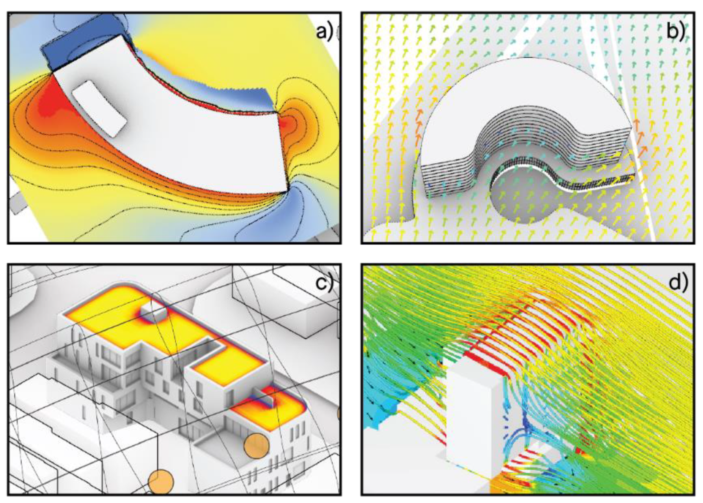
A range of software and plugins are available for modelling microclimate variables (

Table 1. Summary of the software discussed in this paper and their capabilities.

Software	Capabilities	Example Outputs
Ladybug v0.0.68 (www.ladybug.tools)	Weather data visualization, sun paths, solar irradiance simulations	Hours of direct sunlight, solar irradiance
ENVI-met v4.4.3 (www.envi-met.com)	Computational fluid dynamics (CFD) microclimate simulations, outdoor thermal comfort quantification	Air temperature, wind velocity, humidity, mean radiant temperature
SimScale (www.simscale.com)	CFD wind flow simulations, wind comfort simulations	Wind velocity, Davenport wind comfort criteria
Eddy3D v0.3.6.3 (www.eddy3d.com)	CFD wind flow simulations	Wind velocity, Universal Thermal Climate Index (UTCI) pressure coefficients on building facades

). Commonly used tools include Ladybug, ENVI-met, SimScale, and Eddy3D [9], whose outputs are presented in Figure 1. A brief description of these software follows.

Ladybug is an open-source environmental analysis plugin for Grasshopper, the visual scripting interface for Rhino [10]. Ladybug includes several components for weather data visualization and solar radiation simulations. The latter functionality is powered by the Radiance program, one of the most widely adopted and appreciated tool for lighting modelling, which was developed at the Lawrence Berkeley National Laboratory (LBNL) [11]. By merit of it being a plugin, the information produced by Ladybug can directly inform the 3D geometry of the design.

ENVI-met is a holistic, computational fluid dynamics (CFD) microclimate simulation software for modeling surface–plant–air interactions in urban environments. Among the current list of tools, it is the only one capable of simulating the wind flow around buildings; heat transfer at building surfaces; evapotranspiration; and the reflection, transmission, absorption, and emission of solar radiation altogether. Wind flow is modelled using Reynolds Averaged Navier–Stokes (RANS) equations, and radiative fluxes are resolved using an Indexed View Sphere (IVS) scheme. The spatial resolution of simulations in ENVI-met typically ranges from 1 m to 5 m, and the temporal resolution of the output is by default hourly, although turbulence and radiative fluxes are updated at the scale of seconds. These capabilities have been tested and validated in the literature [12,13], making ENVI-met a widely selected software, especially within the research community. A trade-off of its comprehensiveness is the ensuing compute times—in fact, a whole-day simulation can easily take 24 hours or more to complete even on a high-performance computer. Two Grasshopper plugins, lb_envimet and df_envimet, enhance the feasibility of ENVI-met as a complement to the architectural design process [14,15], but their diffusion is still limited.

SimScale is a cloud-based CFD platform capable of rendering annual wind comfort and transient wind flow around buildings. While it can load geometry from CAD programs, results cannot be projected back into them, so this software also remains limiting. Among the advantages of SimScale is the fact that the computing times for annual simulations are fast enough to permit multiple studies in a day. This allows the identification of several critical conditions over the year to allow a deeper understanding of the implication of multiple design options over longer periods of time.

Eddy3D is an airflow and microclimate simulation plugin for Grasshopper [16]. It is powered by the OpenFOAM solver and uses EPW weather files to predict annual wind comfort. The analysis is accelerated by “binning” the EPW wind directions into larger sectors and interpolating the local wind velocities based on wind reduction factors. The results are highly customizable in Grasshopper and Rhino, enabling fine control over visualizations.

3. Methods for the Microclimate Analysis of Architecture Projects

3.1. Boundary Conditions

The meteorological boundary conditions of a simulation refer to the set of physical variables used to initialize or force the numerical model. For example, a list of air temperatures might describe the hourly condition at the inflow boundary of a microclimate simulation. In a research paper, it is common to test an intervention against a single meteorological boundary condition, such as a hot summer day [17,18]. In contrast to scientific studies, in design applications it is critical that the boundary conditions used for architectural microclimate analyses are representative of the project location throughout the year, and all the conditions a site may experience in a year should be accounted for and presented to the client. This means that testing the multiple diurnal temperature and humidity cycles, wind speeds, wind directions, and cloud conditions which are typical for the location being studied becomes fundamental, while the resources (both temporal and economical) for slow simulations are rarely available.

Common choices for validated typical weather data are Typical Meteorological Year (TMY) files, which are produced by several government agencies and made available in the universal Energy Plus Weather File (EPW) format. These hourly, year-long datasets are made by concatenating the individual months of weather station observations chosen for their representativity. While TMY files can be used unabridged in building energy models, the computational intensity of CFD microclimate models usually prohibits year-long simulations. Thus, it is necessary to parse these files for shorter yet still representative periods. Moreover, CFD simulation require user skills and the use of adequate mesh, numerical schemes, turbulence models, and many other details to provide solid information and allow the critical interpretations of the results.

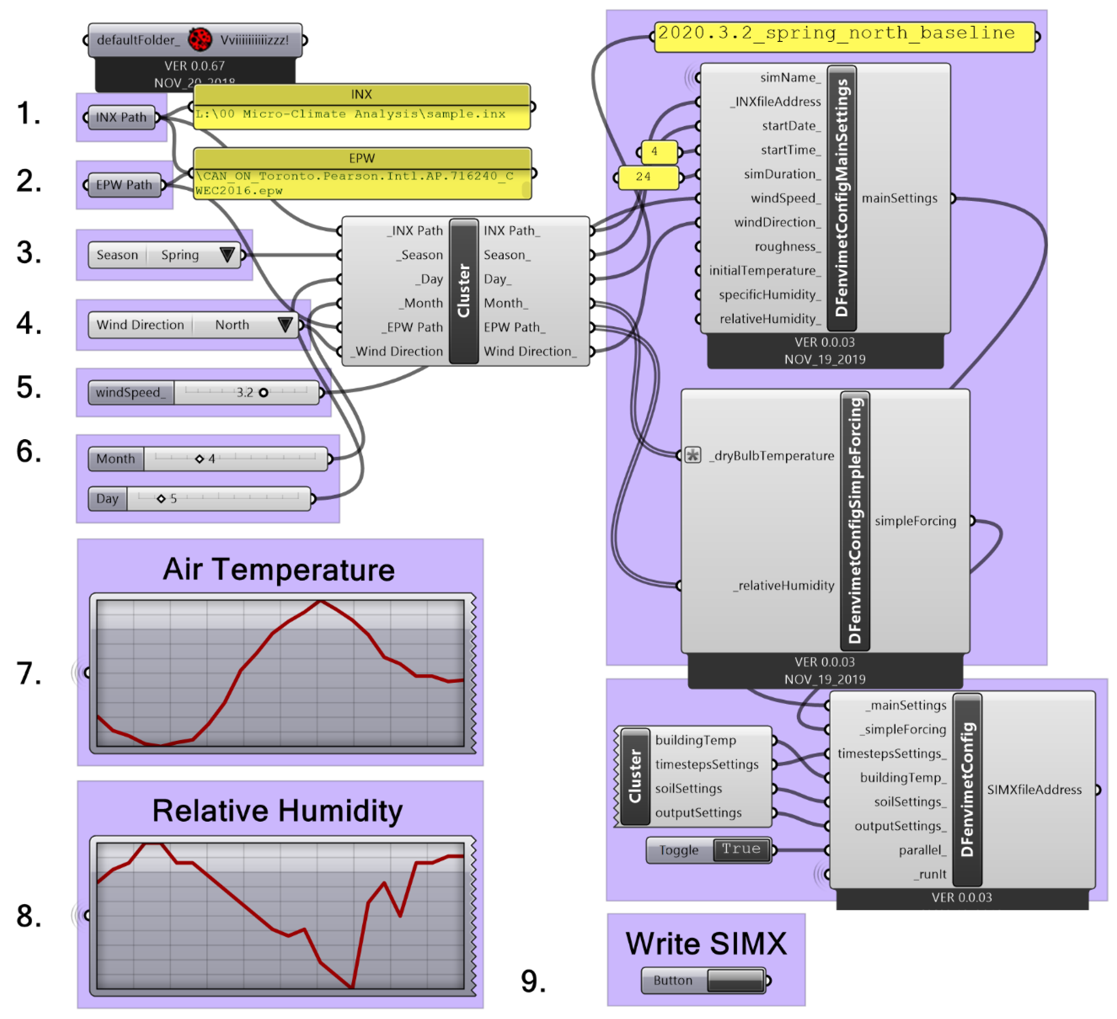
A tool that helps streamline this process is the Read EPW component of Ladybug, which can be used to scrub through the lines in an EPW file while dynamically plotting the relevant meteorological variables. Through this approach, typical fall, winter, spring, and summer days can be quickly distinguished from anomalies. More importantly, the selected hourly data for which to run a simulation can be written directly to an ENVI-met configuration file through df_envimet. This makes it possible to queue up dozens of combinations of boundary conditions in an efficient semi-supervised fashion way. For example, using these components, Figure 2 shows a Grasshopper script, which generates an ENVI-met configuration file for eight wind directions for each season in the location of interest. Further parameters that can be manipulated include the assumed roughness length of the site, which is used to construct the vertical wind profile at the model inflow boundary according to the EPW wind velocity measured at a 10 m height. The script is quicker than negotiating the default ENVI-met user interface, thereby encouraging the consideration of all possible boundary conditions.

3.2. Extracting Results

Complementary to the need to set up simulations rapidly is the ability to handle their results efficiently. When several iterations of a model are being compared, it becomes extremely useful in daily consulting practice to have an automated means of parsing the results. For this, it is possible to benefit from the use of NetCDF, Python, and Jupyter Notebook.

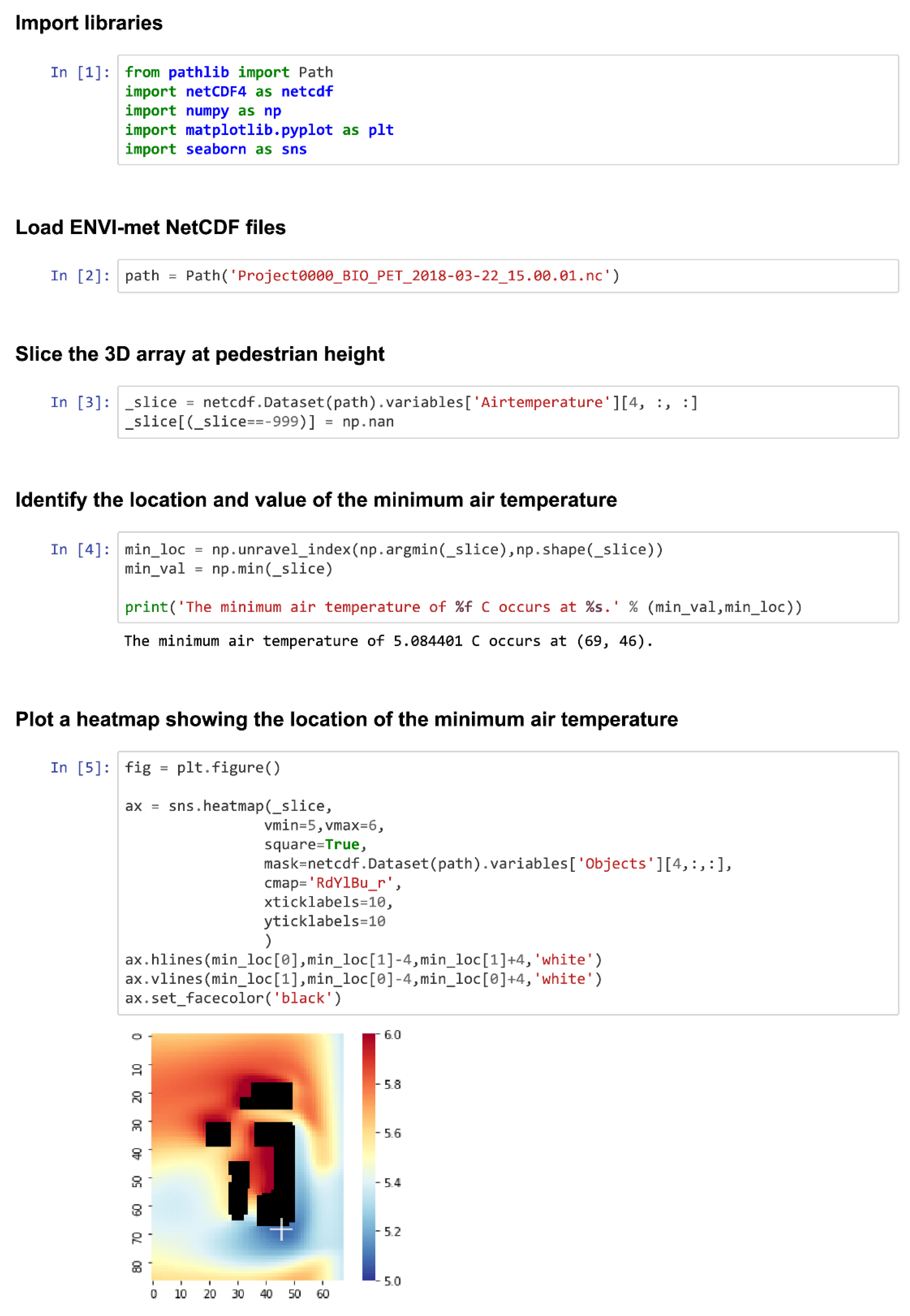
NetCDF (Network Common Data Form) is a self-describing data format developed by UCAR/Unidata, which is used for accessing and storing array-orientated scientific data. It is one of the output formats supported by ENVI-met and has a Python programming interface. Using this module, it is possible to load the hourly 4D (x, y, z, meteorological variable) results from ENVI-met into a 3D NumPy array. From this array, locations of interest can be extracted (i.e., vertical slice at 2 m height) and a range of specialized graphs and statistics can be produced with a few lines of code.

For example, the location of the maximum simulated air temperature can be reported for each scenario (Figure 3), or a time series plot of air temperature at the same location across multiple scenarios can be produced (Figure 4). Furthermore, if additional scenarios are simulated, minimal effort is required to incorporate their results into existing graphs and statistics. This encourages a recursive approach to microclimate simulations.

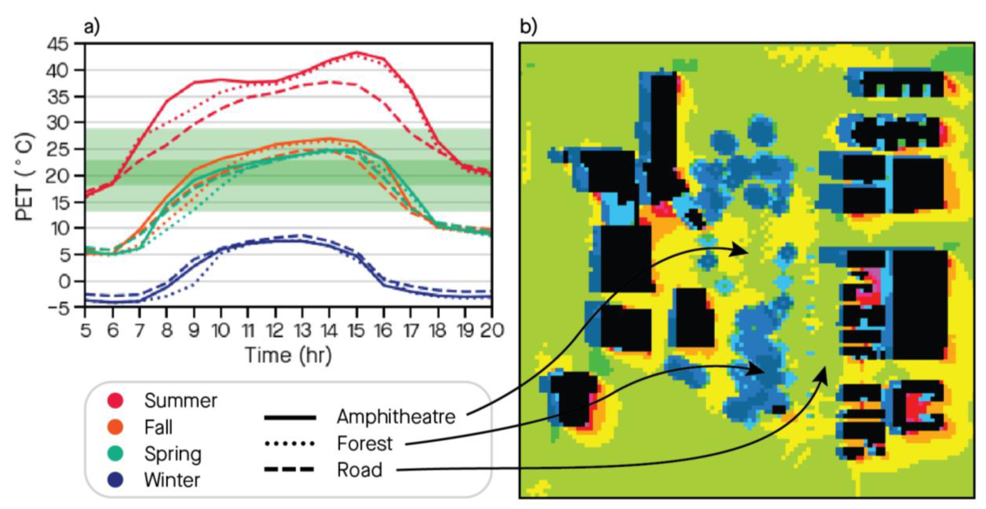
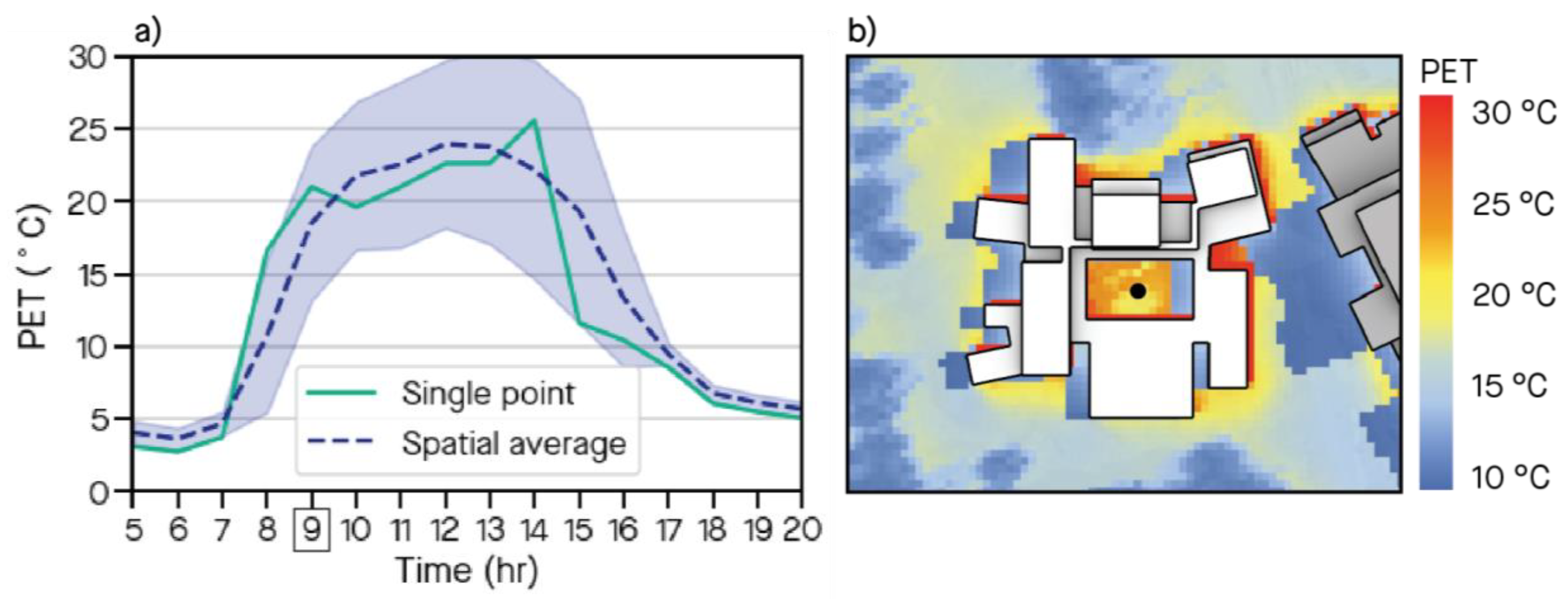
Another benefit of using Python to parse ENVI-met results is that plots can be created for a spatially averaged subset of the model domain. In contrast, the software packaged with ENVI-met only allows a single point to be plotted at a time. Point observations can be problematic when looking at variables incorporating radiation (i.e., mean radiant temperature), which vary considerably across short distances due to the shading of direct solar radiation (Figure 5). By taking the spatial average of these variations, the misrepresentation of an outdoor space’s hourly performance can be avoided. Moreover, spatial averages partially acknowledge that a person may change their position within an outdoor amenity to find better (or worse) thermal comfort.

3.3. Human Thermal Comfort Indices

While the meteorological outputs of a microclimate simulation are important for understanding the underlying physical processes, other metrics exist to provide more human-centric assessments of outdoor thermal comfort. HTCIs relate a given of air temperature, humidity, mean radiant temperature (MRT), and wind speed to a human physiological response, which is subsequently transposed to a single perceived temperature. HTCIs also consider clothing insulation and the metabolic rate of an individual. Two commonly used HTCIs are the Universal Thermal Climate Index (UTCI) and Physiological Equivalent Temperature (PET) [19,20]. UTCI is well suited to high-level assessments because it assumes a fixed metabolic rate (walking, 4 km/h) and automatically adjusts the thermal resistance of clothing based on the provided meteorological conditions. A limitation of UTCI is that it does not accept wind speeds slower than 0.5 m/s, which occasionally results in null values around buildings. PET does not suffer from this limitation, making it preferable for microclimate simulations. Moreover, PET allows for the customization of an individual’s metabolic rate and clothing, thereby encouraging analyses that are tailored to the intended use of space. The formulas for PET and UTCI have been translated to Python in the source code for Ladybug. These scripts can be used independently of microclimate simulations to gain a sense of the consequences of an architectural intervention quickly. 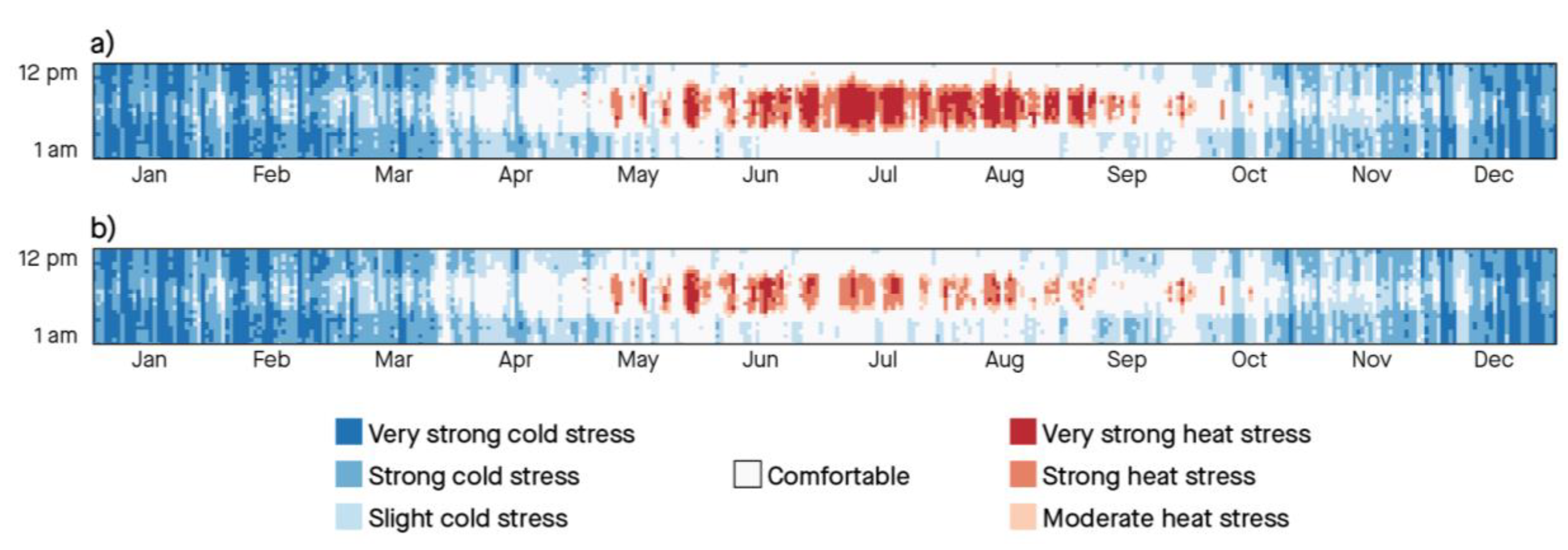For example, Figure 6 shows a graphical way to answer the question “what would the UTCI be if this canopy is expected to lower the MRT by 17 °C?”. The figure helps with understanding the effects of the assumed interventions throughout the year, provides a graphical indication of how the UTCI evolves, and, finally, shows how the annual comfortable duration is increased by 5%.

To definitively assess a design in terms of microclimate, it is important to consider the thermal comfort of space for the entire period of use as opposed to just a point in time. This is met by dynamic, time-integrated metrics. For example, in climate-based daylight modelling, daylight autonomy (DA) is a metric used to describe the percentage of the occupied times of the year when the minimum illuminance requirement is met by daylight alone [21]. By the same token, Outdoor Thermal Comfort Autonomy (OTCA) is a metric used to describe the percentage of occupied times of the year during which a designated area meets a set of thermal comfort acceptability criteria [22], as per the formula:

$$OTCA=\frac{1}{N}\frac{1}{n}{{\displaystyle \sum }}_{k=1}^N{{\displaystyle \sum }}_{h_r=h_i}^{h_f}T{C}_{k,hr},$$

(1)

where $N$ is the number of occupied days, $n$ is the number of occupied hours, $h_i$ is the initial occupied hour, $h_f$ is the final occupied hour, and $T{C}_{k,hr}$ is the result of a thermal comfort acceptability criterion. The criterion itself is defined by:

$$T{C}_{k,hr}=\left\{\begin{array}{c}1 if A_{lower}<HTCI<A_{upper} \\ else 0\end{array}\right\},$$

(2)

where $HTCI$ is the HTCI value at a given hour, $A_{lower}$ is the lowest value of HTCI that is considered comfortable, and $A_{upper}$ is the highest value of HTCI that is considered comfortable. These upper and lower bounds can be defined by PET or UTCI assessment scales. For example, an OTCA calculation based on PET would count the duration for which a space is between 18 and 23 °C PET (equivalent to no thermal stress). Alternatively, less stringent criteria can be used for outdoor circulation spaces where the duration of exposure is shorter.

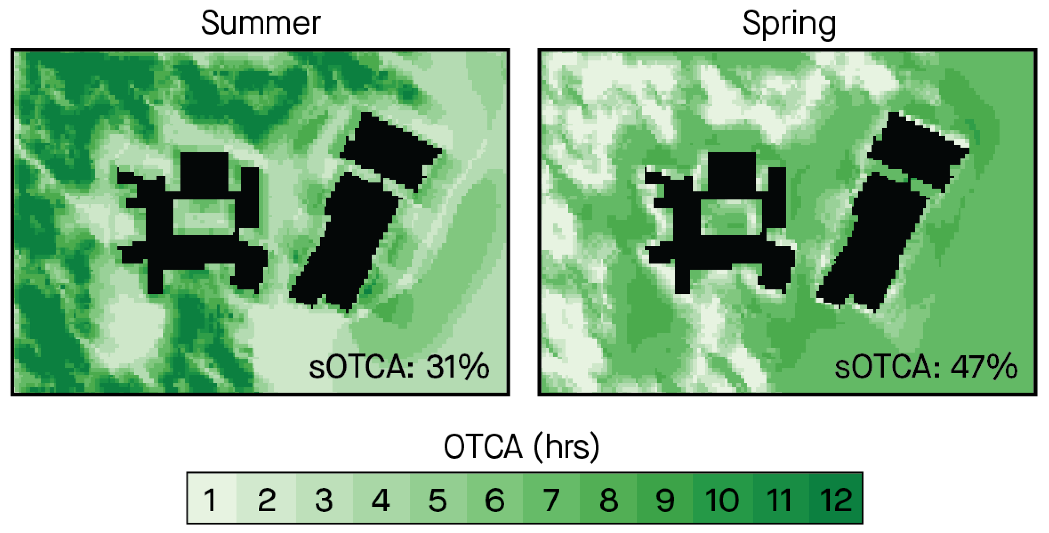
OTCA is not currently a feature offered by ENVI-met, so the authors created a Python script that post-processes its results via the NetCDF library for Python [23]. In addition to producing OTCA heat maps, the script is also capable of reporting Spatial Outdoor Thermal Comfort Autonomy (sOTCA), which describes the percentage of a designated area which meets the thermal comfort acceptability criteria for at least 50% of the occupied period [22]. Used in combination, OTCA and sOTCA form the basis for the rapid and comprehensive assessment of outdoor space (Figure 7). Further, they offer a simplified means to track the incremental improvement of design. A limitation of the current approach to calculating OTCA is that representative seasonal days are used in place of an actual year’s worth of simulations. Recent studies have suggested that the results of annual daylight simulations can be adequately captured by as few as three representative conditions [24], and likely the same concept of principal components can be extended to microclimate analysis.

3.4. Synergistic Applications of Tools

Extensions of analysis tools into the architectural design space have been made possible through open-source platforms like Grasshopper and Dynamo, which continues to expand as the tools become more widely implemented in practice. These platforms add a tertiary informational layer into more traditional CAD and BIM software. Still, computers are not good at open-ended creative solutions that are still reserved to the operator. However, an increase in interest has emerged to expand the possibility of automation to save time doing repetitive tasks, such as iterating design options with slight formal or material changes through the same analysis. For increasing the level of automation in climate modelling, tools for generative design such as Galapagos and Octopus, both of which plug into Grasshopper and Dynamo, are being added to the designers’ toolset [25]. Generative design software allows for targets to be set based on the performance of a model as changes are made to the input parameters. A simple example of this would be the increased area on a wall being observed as the length of it grows. In terms of optimization for microclimate analysis, one could imagine several parameters (the height, width, and depth of an opening, for example) effecting the observed solar radiation on that same wall. This target value is referred to as the fitness, while the control parameters are the genomes. A generative solver combines countless combinations of values for the genomes, outputs a result that is comparable to the baseline fitness, and refines it as it solves for successive generations in an attempt to either maximize or minimize the target; Figure 8 shows the genomes and fitness process in Galapagos.

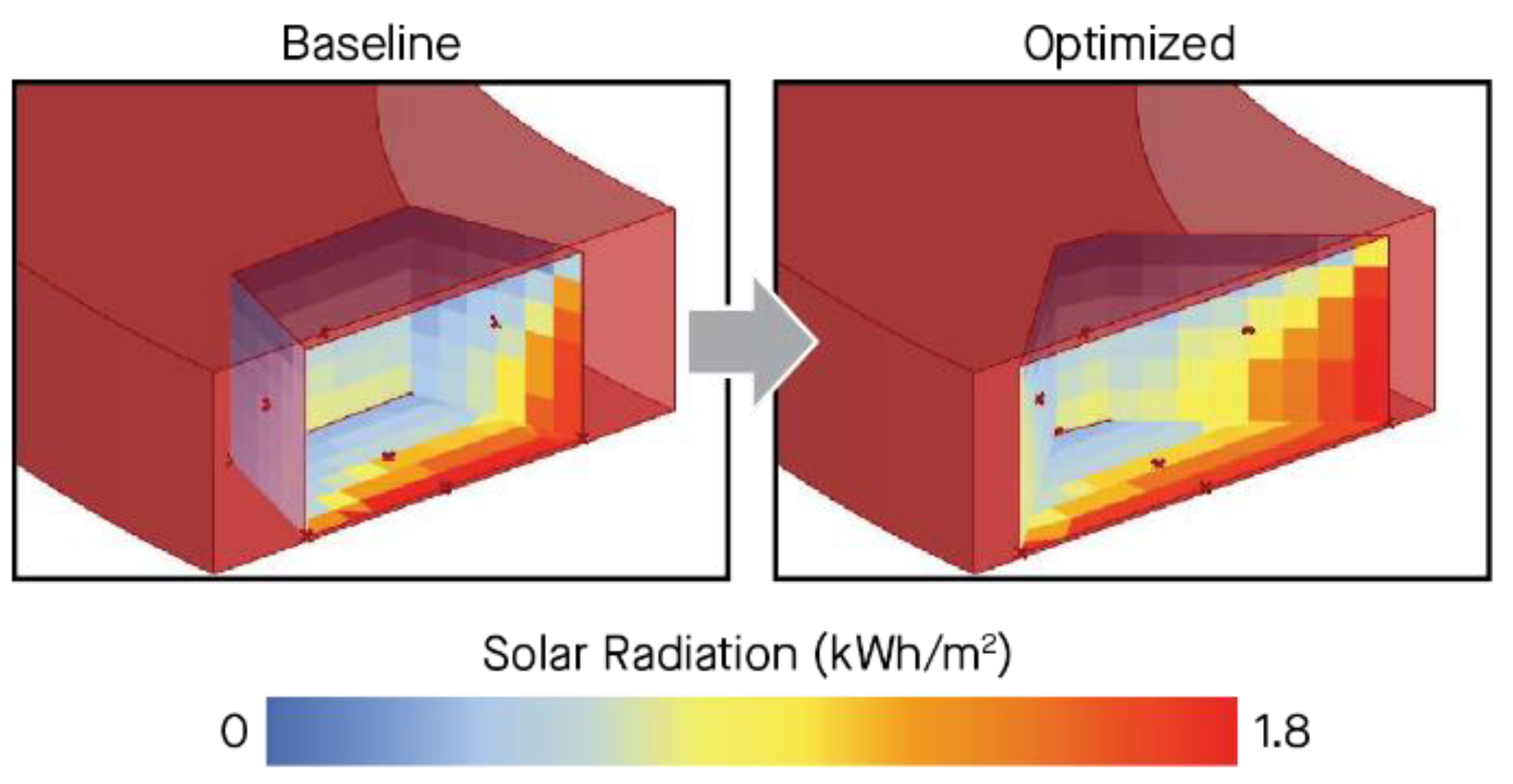
Another automated possibility for design generation is showed below. Here, the authors tried to reconcile a maximized solar radiation on an upper-level balcony with the dimensions and orientation of that terrace in order to extend the OTCA into the shoulder seasons. The goal was to maintain roughly the same location and size for the balcony, while allowing to the walls to move and rotate slightly. The top-performing options in this study increased the solar radiation by more than 50% in the shoulder season when compared to a baseline conceptual design (Figure 9). The final step involved a visual check with the designers to determine which forms would satisfy the plan requirements.

While the presence of a dynamic and automated design process increases, it is largely misconceived that these tools eliminate or replace the designer in the creativity process. In fact, the selection of which tool, metric, and support for architecture creativity is a consideration that is directly tied to design today. The capacity to rapidly generate and prototype architectural form in 3D design spaces enables architects to be both pragmatic and precise in their processes. This is achieved by a link that is established between formal decisions and human-centric evaluations based on analysis rather than mere speculation or automatic processes.

It should be acknowledged that with the increased capacity to synthesize analysis software with automation, there are emerging questions around the validity and substantiating of claims made by design teams engaging in climate-sensitive design. The ability for designers to cherry-pick biometeorological data that supports their research and omit others that do not can lead to a distortion of data in the interest of a convincing architectural narrative. Currently, there is no regulatory oversight that would ensure practices in microclimate analysis integration in design processes are authentic or are being done responsibly.

3.5. Design Interventions

The efficient and synergistic use of simulation tools is only part of the effort required to incorporate microclimate as a design driver of architecture. Equally relevant to this discussion is the process of linking simulation results to design interventions. This occurs in three steps: recognizing the type of thermal discomfort, zeroing in on the environmental parameters causing that discomfort, and designing interventions that manipulate those environmental parameters. For example, if a simulation reveals a prevalence of cold stress in an outdoor patio during a mostly comfortable season, possible culprits are the wind (which controls the rate of convective cooling on individuals’ skin) or the MRT (which determines the radiative heat balance between an individual and the environment). With this knowledge, an architect may choose to add wind-blocking landscape features while rearranging the building massing to allow more direct sunlight onto the patio. Alternatively, this analysis may reveal a naturally more comfortable location for the outdoor amenity.

A summary of design interventions and the simulation results that may warrant them is provided in

Table 2. Simulation results and corresponding design interventions.

Simulation Result	Environmental Parameter	Desired Change	Design Interventions
Heat stress	MRT	decrease	Trees shading canopies/pergolas refine building massing/orientation to increase shade
	wind speed	increase	refine building massing/orientation to channel prevailing winds
	air temperature	decrease	evaporative mist-spraying systems; vegetation cool materials
Cold stress	MRT	increase	Refine building massing/orientation to increase sun exposure

. Most of the interventions listed directly influence MRT and wind speed, which have a significant impact on thermal comfort. While more strategies are currently under investigation in scientific literature, some are less efficient or practical at the scale of an architectural project. For example, water ponds must be large to create a noticeable cooling effect [26]. Green roofs, while having energy and drainage benefits, tend to have minimal impacts on the temperature at ground level [27,28].

Recent work by designers suggests that novel opportunities for microclimate enhancement exist in the form of dynamic devices that adapt to changing climate and occupancy conditions. In Toronto, a team of architects, climate engineers, and urban planners studied the effectiveness of “weather mitigation systems” consisting of various Ethylene tetrafluoroethylene (ETFE) structures designed to retract, collapse, and relocate to provide varying levels of shade and wind dampening depending on the season [29]. In London, the Elytra Filament Pavilion attempted to relate people flow to microclimate conditions using real-time measurements of movement frequency and UTCI at an array of positions beneath a robotically constructed canopy [30]. This experiment foretells of data-driven architecture which continuously refines itself to provide the greatest number of people with the highest level of thermal satisfaction. These examples showcase new opportunity for spatio-temporal variation in microclimates that is controlled using simulations with a precision that simple canopies, trees, and windbreaks are unable to match.

4. Conclusions

This paper discussed the challenges and experiences while implementing microclimate analysis tools in architectural design practice. The study revealed and made evident that the existing toolset—in particular, ENVI-met—requires significant adaptation when used for such purposes. A handful of plugins and open-source code could assist with this process and was presented by the authors. The primary benefits of these add-ons are improved software interoperability, the rapid development and analysis of simulations, and the ability to calculate new and emerging metrics such as OTCA. Nonetheless, there is progress to be made before microclimate can become a thoroughly integrated design driver of architecture.

It should be noted that the microclimate analysis activities described in this paper are not intended to replace services obtained for safety and compliance purposes, such as wind tunnel testing. Rather, the study proves the feasibility of unlocking microclimate as a basis for site-specific and climate-driven design and as a means to improve the year-round experience offered by outdoor amenities.