Article

Indoor Temperature Validation of Low-Income Detached Dwellings under Tropical Weather Conditions

by
R. Alexis Barrientos-González
1,
Ricardo E. Vega-Azamar
1,*,
Julio C. Cruz-Argüello
1,
Norma A. Oropeza-García
2,
Maritza Chan-Juárez
1 and
Danna L. Trejo-Arroyo
3
1
Tecnológico Nacional de México/I.T. Chetumal. Insurgentes 330, Chetumal 77013, Mexico
2
División de Ciencias e Ingeniería, Universidad de Quintana Roo. Boulevard Bahía s/n esq. I. Comonfort, Chetumal 77019, Mexico
3
CONACYT-Tecnológico Nacional de México/I.T. Chetumal. Insurgentes 330, Chetumal 77013, Mexico
*
Author to whom correspondence should be addressed.
Climate 2019, 7(8), 96; https://doi.org/10.3390/cli7080096
Submission received: 6 July 2019 / Revised: 22 July 2019 / Accepted: 23 July 2019 / Published: 2 August 2019

Abstract

:
Urban territorial expansion generated in the last decades has brought a series of consequences, such as the variation between urban and suburban weather conditions affecting indoor temperature and increasing electricity consumption derived from the use of cooling systems. Current approaches of simulation models in residential buildings use indoor environmental data for carrying out validations to propose hygrothermal comfort alternatives for the mitigation of the effects of the external environmental conditions on the interior spaces of dwellings. In this work, an hourly evaluation of both indoor and outdoor environmental parameters of two case studies in a tropical climate was carried out, by means of a whole-building simulation approach tool during a week representative of the warmest period of the year. The integration of the collected environmental data in the theoretical model allowed us to reduce the error range of the estimated indoor temperature with results in normalized mean bias error between 7.10% and −0.74% and in coefficient of variation of the root mean square error between 16.72% and 2.62%, in the different indoor zones of the case studies. At the same time, the energy assessment showed a difference of 33% in Case 1 and −217% in Case 2 for final electricity consumption.

1. Introduction

Between 1995 and 2015, private housing in Mexico registered a growth of 39.2% [1], mainly due to policies promoting the acquisition of private housing through labor and social credit systems [2], while detached dwellings represent 84% of total social housing in cities with a population greater than 100,000 inhabitants [3]. Low-income housing development has led to urban problems, such as territorial expansion towards the peripheries, infrastructure deficiency [4], greater mobility rates, increased electricity consumption and modification of the urban microenvironment. Although the latter may be attributed to global warming to a greater extent, it has been recorded that temperature variations within urban settlements can reach an additional 4 °C between urban and rural and peri-urban areas; this phenomenon has been widely studied under the name of urban heat islands (UHIs) [5] which derives from being detrimental for outdoor comfort and building energy impacts [6]. In addition, massive construction of housing in countries like Mexico is characterized by the indiscriminate repetition of design patterns throughout the territory, regardless of the conditions of each climate zone, with warm regions being the most affected by higher energy consumption derived from the conditioning of indoor spaces by cooling equipment, which represents 19.6% of the energy used [7]. Mexico’s National Meteorological Service points out that the country is composed of four main climatic regions: arid, dry tropic, temperate and humid tropic; where both the arid and the humid tropic present the highest percentages of air-conditioning equipment use for housing with 51.9% and 21.2%, respectively [8]. For its part, the National Housing Commission has implemented recommendations included in the National Appropriate Mitigation Actions (NAMA) for Sustainable Housing [9], mainly focused on energy efficiency as the optimization parameter; however, indoor temperature is also one of the most important indicators to understand a house’s thermal performance, which takes into account the influence of the external environment, the internal loads and the dwellers, allowing the study of hygrothermal comfort and optimization measures to counteract radiation and heat conduction effects on the building envelope, and the calculation of the cooling systems capacity. Table 1 shows the main acronyms used throughout the work.
Building simulation models are tools used to evaluate overall performance, whose use at the initial design stage is focused primarily on evaluating the lowest final consumption: electricity, gas and water [10]. In recent years, indoor temperature has been considered an evaluation parameter in law-driven simulation models and, as it occurs with energy models, they present a documented gap error when compared to real performance during the post-occupation period [11,12] due to several factors, mostly identifying as key parameters the temperature variation in the region and the occupants’ behavior at the dwelling operation stage. This has led to the adoption of a validation approach of simulation models whose main objective is the reproduction of the overall performance of the building to evaluate its evolution throughout its life cycle or to compare the outcomes that would be obtained by different constructive alternatives.
Therefore, in order to compare improvement proposals for thermal performance in low-income housing under tropical weather conditions, the main objective of this research was to assess the magnitude of the influence of microenvironment conditions for the creation of a theoretical model that keeps a real approximation of the thermal performance at the dwelling multi-zone level of two occupied detached social houses through a whole building simulation approach, validated at an hourly basis for indoor temperature. The present study is divided into three parts: the first part presents a brief review of the literature on model validation with environmental data, a second part describes the methodological process, as well as the tools and equipment used for data collection, and the third part presents the results of the monitoring campaign processed data and the discussion of the results.

2. Literature Review

A large number of studies have been conducted through the validated simulation approach focusing, primarily, on a detailed record of energy consumption data including those from heating, cooling and other internal loads, and taking into account indoor temperature monitoring as the “final tune” parameter [13,14]. On the one hand, UHIs have been identified as a mayor phenomenon affecting urban areas, in which air temperature variation is the most relevant factor affecting both thermal comfort and building energy use [15], where decrease of precipitation and a large number of days without rain tend to intensify temperature rising in tropical weather cities [16].
On the other hand, Tisov et al. refer to indoor air quality evaluation, in which temperature and relative humidity play a central role, as barely studied due to the amount of data required and the process for the analysis [10]. Although there is no specific standard procedure or guidelines to validate indoor temperature, several authors have chosen to take the American Society of Heating, Refrigerating and Air-Conditioning Engineers (ASHRAE) guidelines 14-2002 as a reference for energy consumption criteria to perform environmental assessments [17].
As a general criterion to reduce the gap in model simulation, several authors recommend the incorporation of environmental data from the specific study site by installing a weather station, in order to create an actual meteorological year file or a customized weather file [12]. In cases where this is not possible, other authors propose to start from historical meteorological files to predict the increase in temperature or obtain reliable data by interpolating with data from nearby stations [18]. For the case of housing, it has been documented that models validated through environmental data gathered on site have been executed with good results, without limiting its application to just one single type of climate. In Denmark, Paliouras et al. carried out a theoretical model calibration of a house under passive ventilation and heating standards in a post-occupancy period, recording hourly data in a 30-day period in each zone of the dwelling [19]. The study took the minimum and maximum average of daily temperature of each studied zone which was contrasted against the simulated averages. For the calibration of the model, six iterations were carried out manually, modifying input parameters obtained from detailed interviews regarding the operational activities during the monitoring campaign. On the other hand, in Bolzano Italy, an energy validation of a 13th-century dwelling was conducted, incorporating input data obtained from the study site, such as real envelope conductivity, air permeability and external environment [20]. By performing the calibration processes for different seasons, a root means square error (RMSE) of 0.96 K was achieved in the initial model, while in the first calibration, these authors reached 0.66 K and 0.62 K for summer and winter data accuracy, respectively. In America, Osma-Pinto carried out a housing model validation in Bucarama, Colombia, taking as reference the indoor temperature registered in different spaces of an unoccupied house in periods with and without natural ventilation in each zone in order to identify the closest one to the actual registered data. It turned out that the closest benchmark occurred when considering natural ventilation (windows and doors open) with a mean square error temperature value of 0.21 °C, while for no ventilation conditions, a maximum difference of 0.82 °C was obtained for the bedroom. Then, this information was used to evaluate the best orientation scenario [21]. In Ecuador [22], Miño and Naranjo conducted a comparative evaluation between two rural dwellings with different envelope materials such as walls and slabs. In addition to the comparison between outdoor temperature impact to that recorded indoors, the model’s accuracy was evaluated with hourly data from the monitoring at two levels of evaluation; in a last level the correlation error was reduced by iterations varying the levels of infiltration, identifying the correlation between observed and predicted data as 0.89 for compressed earth block and 0.94 for hollow concrete block, with a RMSE close to 1.1 °C in both studied dwellings. On the other hand, in the Dominican Republic the validation of a dwelling model during the warmest week in June was conducted through the use of indoor environmental sensors, including wall temperature, in order to evaluate different improvement alternatives such as orientation, eave lengths and roof isolation alternatives to improve of thermal comfort [23].

3. Methodology

The procedure chosen to carry out the model validation was based on the Hwa Cho and Sook Kim methodology [24] simplified in Figure 1. The process started with dwelling selection to continue with a detailed description through an audit evaluation that allowed the creation of the theoretical model (TM). Environmental data (temperature and relative humidity) were recorded in sub-hourly periods by data-acquisition devices in each of the houses different zones, which was the actual performance (AP). Then, all records were compared with the TM output data taking into account the operating temperature, because that includes both air temperature and radiant temperature of the walls. The calibration process consisted in the integration of the environmental data through a customized meteorological file and the running of several iterations until achieving the compliance range of the ASHRAE 14–2002, which, based on the statistical analysis, recommends a nominal mean bias error (NMBE) ≤10% and a coefficient of variation of the root mean square error (CV RMSE) ≤30%. The formulas of both indices are expressed in Equations (1) and (2):
N M B E % = 1 m a v . i = 1 n ( ( m i S i ) n × 100
C V ( R M S E ) % = 1 m a v i = 1 n ( m i s i ) ² n × 100
where, n is the amount of data in hours; mav is the mean of the actual recorded data; mi is the actual data and si is the simulated data [25].

3.1. Case Studies

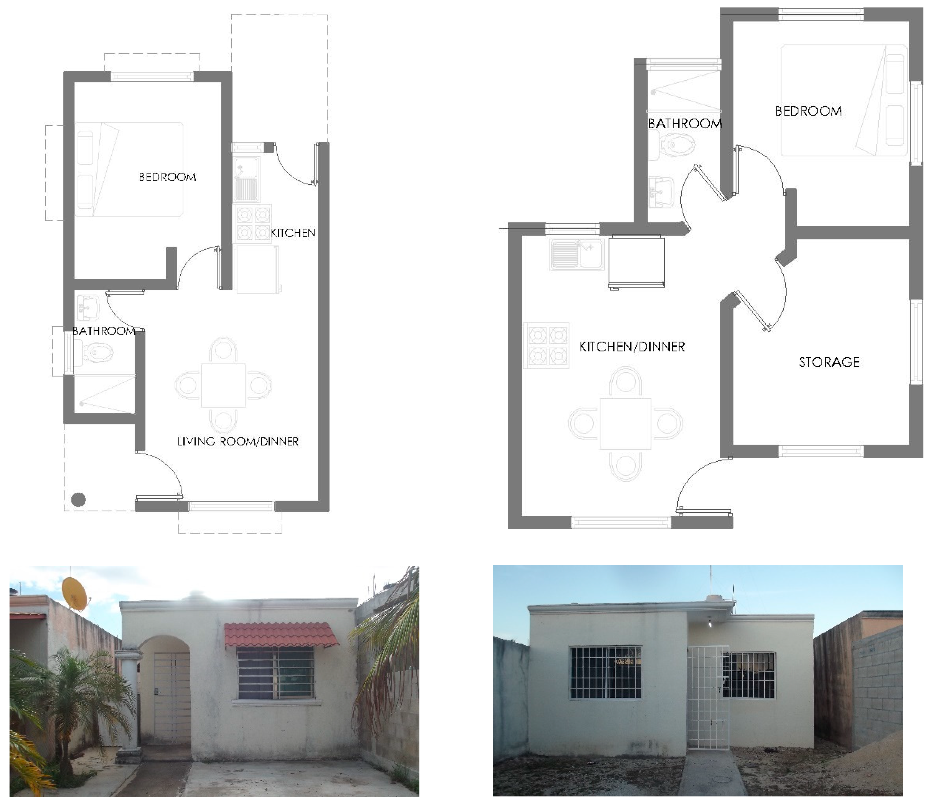
The selected case studies were two dwellings in the city of Chetumal, located south of the Mexican Caribbean state of Quintana Roo, under the coordinates 18°28′ to 18°34′ North latitude and 88°14′ to 88°29′ West longitude, with an average elevation of 9 m.a.s.l. [26]. According to its geographical location, the Köppen classification groups the region within the sub-humid warm zone [27], having an average annual temperature of 26.7 °C [28]. Moreover, the selected dwellings are situated Northeast of the city in a high-density area. Table 2 condenses the characteristics of each case study, while Figure 2 shows the studied dwellings with the spaces comprising them.
Given that both cases have two occupants, the average metabolic factor used was 0.90 [29]. In both cases, the dwellings have an air-conditioning system (mini-split type) with the same cooling capacity; however, for Case 1, it was assigned a power of 1.85 kW since the equipment has been in use for more than five years [30]. Regarding the envelope thermal values, these were identified by the visit to the site, assuming constant thermal properties, as represented in Table 3. With reference to the internal loads, these were calculated by the absolute demand per area proportion, which for Case 1 was 145 W and 310 W in the room and the kitchen/dining room and in the main chamber, respectively, while in Case 2, they were 165 W and 450 W [31]. Also, for the kitchen, the latent fraction was 0.30 for both cases. As for the occupation activities, this was the result of interviews to the occupants and a simplified scheme was made, due to the detailed description. Therefore, at a first stage, dwelling 1 reported unoccupied periods during the week (Monday to Friday) from 8:30 am to 7:00 pm, on Saturdays, it was reported an unoccupied period from 12:00 pm to 9:00 pm. On the other hand, dwelling 2 reported unoccupied periods between 8:00 am to 8:00 pm on weekdays, with unoccupied periods from 10:00 am to 8:00 pm on Saturday. In both cases, Sundays were the days with the maximum occupation period: for Case 1, they reported and absence from 9:00 am to 6:00 pm, while in Case 2, from 12:00 pm to 3:00 pm. In terms of air-conditioning (heating, ventilation, and air conditioning, HVAC), the period of utilization was defined with a total of 44 hours of operation for Case 1, while Case 2 reported a total of 41 hours. Furthermore, for Case 1, the living room/dining room window reported opened 24 hours a day during the 7 days of the week, contrary to Case 2, which reported not opening the windows, not even during the occupation period.

3.2. Equipment and Data Recording

The geometric model configuration was made with DesignBuilder™ software integrated with the EnergyPlusTM calculation engine, developed for the U.S. Energy Department, which has become one of the most reliable tools for estimating indoor temperature, energy use and environmental performance.
For the registration of indoor environmental data, HOBO Onset MX1101 sensors were used. For the placement of the devices, the recommendations of ASHRAE 55-2017 were taken as reference [32], except for the common areas, where these were placed 80cm below the roof level, while in the particular areas it was decided to place them on the partitions, away from direct solar radiation and air-conditioning equipment outputs. All this, in order to not obstruct the occupants activities and avoid damage to the sensors [33]. Two reference monitoring campaigns were performed. First, outdoor environmental parameters were monitored by using a HOBO MX2300 data logger, to obtain both relative humidity and temperature, which are a set of parameters for the microenvironment assessment. The logger was placed inside a high-density polyethylene (HDPE) sunscreen, and located on the dwellings roof during the evaluation week. At the same time, as a part of the macro-environment campaign assessment, records were taken from the meteorological station Davis Vantage Pro installed at the Technologic Institute of Chetumal, which is located 4.5 km from dwellings. The records from campaigns, both the sensor and the meteorological station, were made at intervals of 15 min that were then averaged to obtain the hourly measurement. In addition, the integration of these data allowed the creation of a customized meteorological file, integrated by the temperature, relative humidity, global horizontal radiation, dew point, wind speed and wind direction data recorded by the station.

4. Results and Discussion

4.1. First Evaluation

As a part of a preliminary evaluation, a simulation of the TM, created from the audit description, was run and evaluated against the results of a first indoor temperature monitoring campaign in the bedrooms of both dwellings: for Case 1, the campaign lasted from 9 February to 30 April 2019 (a total of 1944 hours) and for Case 2, it lasted from 10 February to 30 April 2019 (1920 hours). At this stage, the evaluation of the simulations was carried out with the city’s historical meteorological file obtained through Meteonorm. As for the overall energy consumed in both houses, this was obtained by the electric bill issued bimonthly. Since the analysis period did not match with the bill period and the study was conducted during three months, it was necessary to calculate daily consumption through the daily average of energy consumption. Based on that, the first simulation period led to the results presented in Table 4.
Preliminary results, during the first level study, showed a difference in temperature averages simulated at a first level. Taking into account the ASHRAE criteria for the monthly period, where ranges for NMBE and CVRMSE must comply with an index of <5% and <10%, respectively, it can be seen that relative humidity parameter in Case 1 was within the established criteria. As for energy consumption, the theoretical model tended to overestimate energy output data, where Case 2 was identified with the highest gap of 167% over the actual consumption. Due to this difference in the estimations, a second level of assessment was carried out, this time including the environmental results of the remaining zones of the dwellings. The selection of the representative week was made based on a random run of the historical temperature of the city to determine the warmest period. Figure 3 shows the average weekly temperature during a typical year. It can be appreciated that from March to September there is a relative uniformity in temperature, being the months of May, August and September those that report critical values, these months also share the highest electricity consumption, based on the electric bill records.

4.2. Second Evaluation

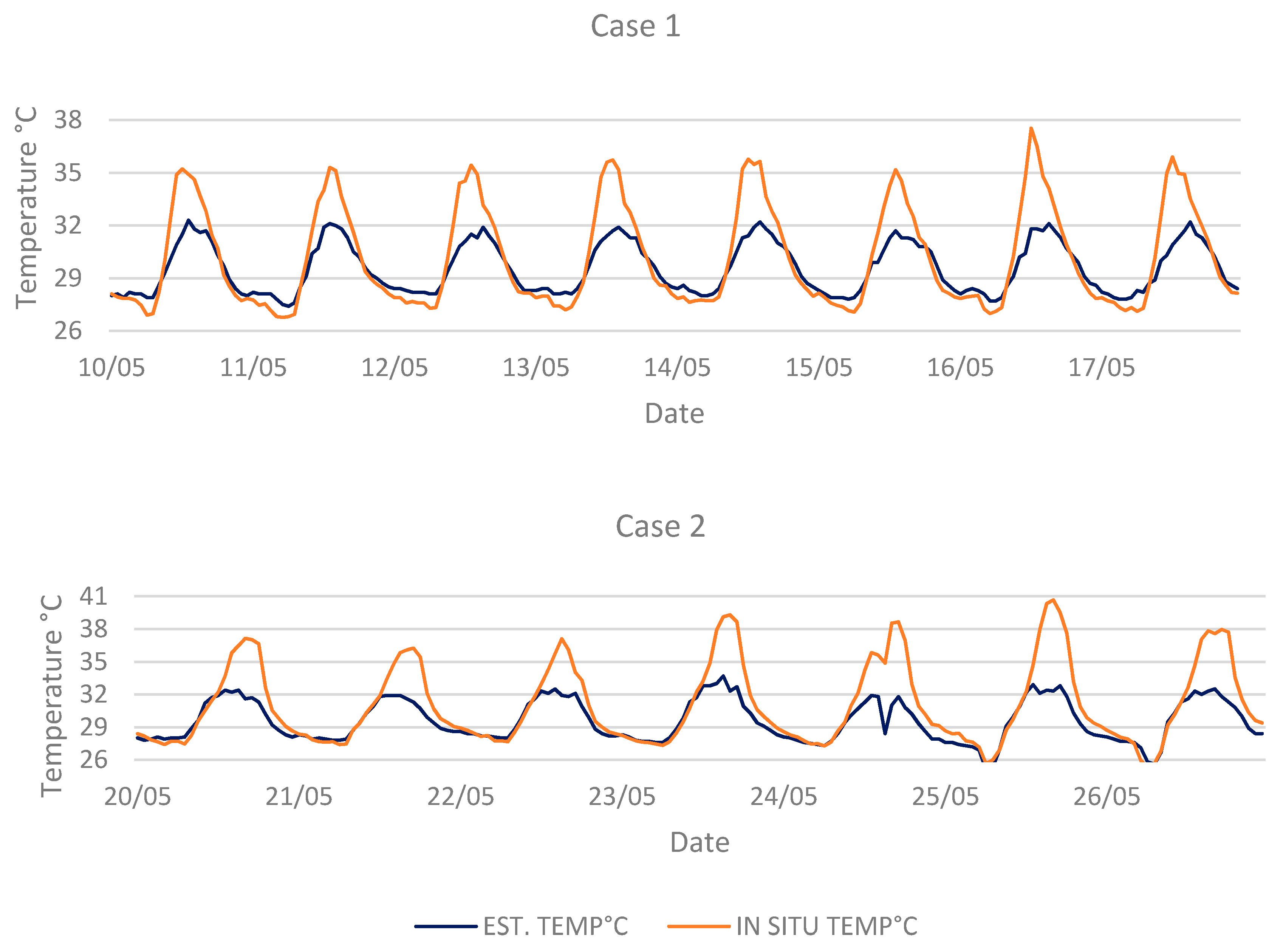
For Case 1, the monitoring campaign was carried out from May 10 to 17, 2019; for Case 2, the evaluated period comprised from 20 to 26 May 2019. Results from the environmental parameters monitoring are shown in Table 5, while a graphical comparison of outdoor temperature can be seen in Figure 4, where the highest temperatures of the microenvironment were recorded, with a maximum difference registered of 5.24 °C and 6.97 °C for Case 1 and Case 2, respectively. On the other hand, the constant maximum relative humidity records are presented for the macro-environment, with a percentage difference of 5.19% for dwelling 1, and 8.07% for dwelling 2.

4.3. Indoor Temperature Model Calibration

To achieve the theoretical model calibration, the data came from a second run of simulations replacing the historical meteorological file with the one corresponding to the current meteorological file. On the other hand, a second round of interviews with the dwellers was carried out to define the day-by-day activities during the period of overall dwelling monitoring. In this level, the occupants of Case 1 reported occupation periods of two more hours during Monday and Friday in relation to the first interview. While on Saturdays, unoccupied period extended from 9:00 am to 8:00 pm, and on Sundays they reported an unoccupied period from 10:00 am to 4:00 pm. Through the same interview, it was found that air conditioning was turned off on average at 6:00 am during weekdays, and at 4:00 am on both Saturday and Sunday, which translates into an increase of 24 hours in air-conditioning.
In Case 2, occupancy remained constant except for air-conditioning time schedule which also reported an increase of 31 more hours per week in contrast to the evaluation in February. In addition, dwelling 2 reported a reduction in the set point temperature to 16 °C during the first 3 hours of ignition, eventually returning to the set point of 23 °C once the room was at a “pleasant” temperature. Results of the model calibration are shown in Table 6.
Infiltration is one of the most complex parameters to measure that may lead to uncertainty. Three infiltration values were evaluated in the second level of iterations for each zone taking as reference the ranges set by the Air Tightness Testing and Measurement Association (ATTMA) Technical Standard, to determine the permeability of the dwellings [34], expressed randomly as 0.20 m³/h.m² at 50 Pa, 0.60 m³/h.m² at 50 Pa, 0.80 m³/h.m² at 50 Pa, for optimal, medium and poor tightness, respectively. The modifications of the infiltration entailed a lesser impact on the simulated indoor temperature, however, greater variations presented for humidity, where the difference between the simulated relative humidity and the actual one came to present a differential error of up to 33%. At the same time, for the case of relative humidity, positive linear correlation values, classified within the moderate to good range (0.3–0.7) [35], were obtained in all the analyzed areas, in particular, for the three spaces without air conditioning.
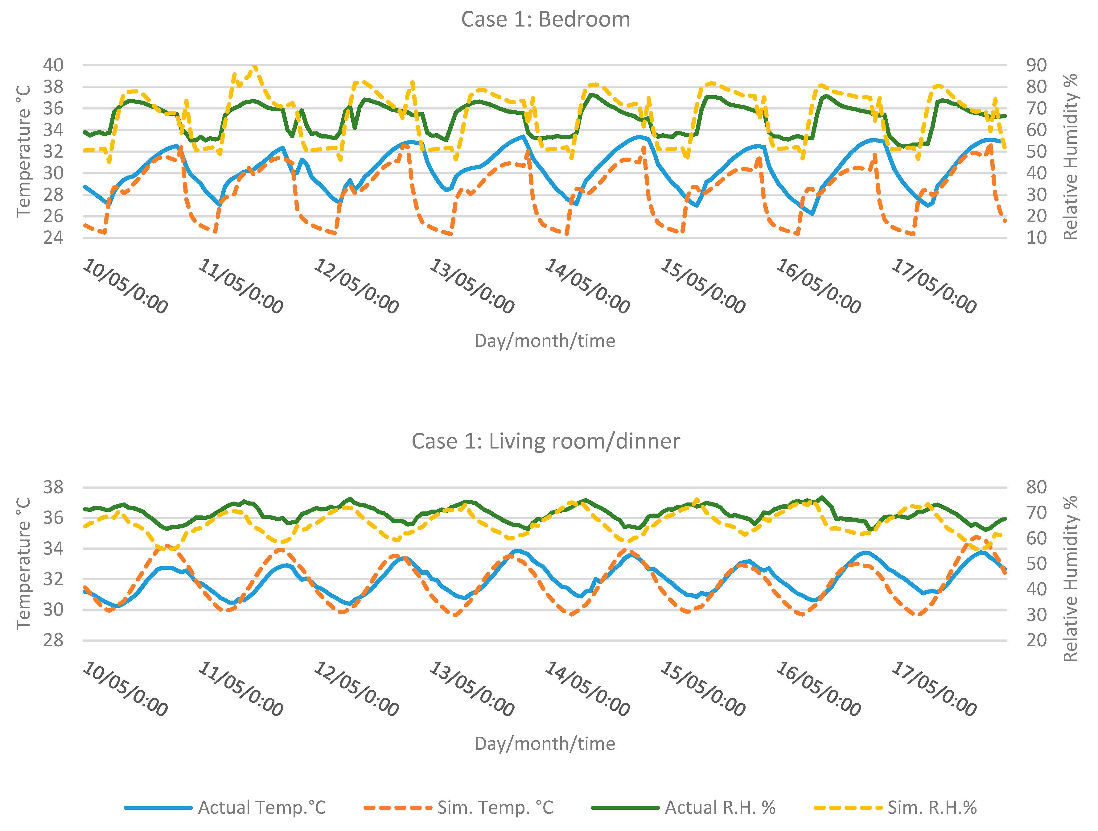
Regarding indoor temperature, a weak dependence (0–0.30) was observed in the first iteration. However, it should be noted that all relative humidity measures values registered indoors were higher than 60%. The main reason for this is the lack of natural ventilation in the spaces preventing air renewal. For the living/dining room in Case 1, that was the only space reported to keep the windows open, corresponding to an average of 2 ren/hr. A graphical representation of the hourly temperature oscillations during the warmer analysis period between actual measured data and results from the optimized iterations is presented by zones for Case 1 in Figure 5.
In Case 2, the average humidity levels differed by 4.73% and 3.12% in the dining room and storage, respectively, which reported windows closed for 6 days a week; this minor variation may be due to the orientation (northeast) of dwelling 2. A graphical representation of the hourly temperature oscillations during the warmer analysis period between actual measured data and results from the optimized iterations is presented by zones for Case 2 in Figure 6. The evaluation allowed the achievement of closer values in those spaces without cooling equipment, reporting differential values and error below compliance since the beginning. From the results obtained in both rooms, it can be seen that, with the second iteration, percentage errors close to 0 were obtained. For the storage in Case 2, the final improvement of indoor temperature achieved only 1.83%. However, from the temperature fluctuations in the graphs, it can be appreciated that EnergyPlusTM tends to underestimate the temperature when considering the internal loads, either from the dwellers or from electrical appliances in operation.
As for the spaces with air conditioning, the coefficients of variation presented an improvement in the prediction of both indoor temperature and relative humidity. In the bedroom of Case 1, the air set-point temperature presenting the best correlation was that corresponding to the iteration with 20 °C which resulted in a value of 0.37, compared to 0.33 and 0.28 obtained with the set-points at 18 °C and 22 °C, respectively. This difference may be caused by the deterioration of the cooling equipment due to the fact that it has more than four years of operation [36]. In the bedroom of Case 2, the dwellers pointed that, during the week. the set-point temperatures used were 16 °C and 23 °C. Results for different set-point values iterations such as 16 °C, 18 °C, 21 °C and 23 °C showed correlation values of 0.38, 0.36, 0.31 and 0.23 respectively. Despite the complexity of evaluating air set-point temperature, it was decided to keep the 16 °C due to the moderate relationship value achieved.
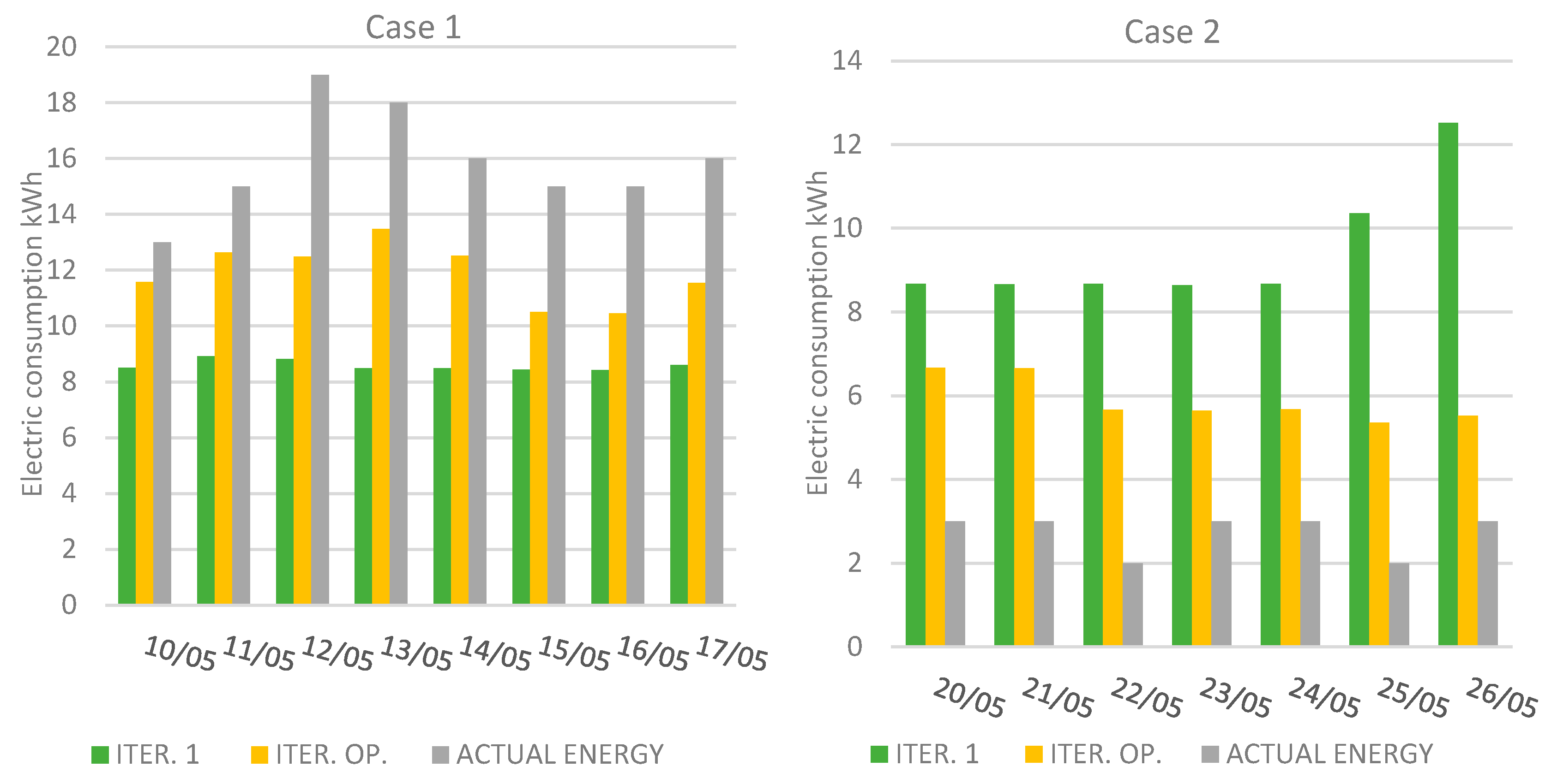
Finally, as a complementary parameter for this work, energy consumption derived from the schedule defined by the dwellers during the first and second evaluation levels allowed the identification of two aspects: a sub-prediction in Case 1 and an over-prediction in Case 2. Figure 7 shows the comparison of daily consumption, which for dwelling 1 presented in the first and in the optimized iteration a difference of 46% and 33%, respectively, with total values of 68.17 kWh and 95.16 kWh, compared to the 127.0 kWh recorded on site. In contrast, in dwelling 2, the weekly electricity consumption was over-predicted when compared to the 19.0 kWh recorded on site; the first iteration was 3.48 times greater than the actual one and, in the second iteration, the gap was reduced to 2.17 times the actual, with absolute values of 66.19 kWh and 41.35 kWh. The electricity bill turned out to be a reference value for the consumption that did not allow the comparison on a daily basis. The daily reading of the electricity consumption meter, complemented with the descriptive reports of home appliances use by dwellers, also failed to satisfactorily approximate the simulated results, since the difference may also be attributed to different causes, ranging from errors in programming and use to electrical interference or physical problems in the installation. Therefore, this evaluation requires the use of adequate sensors for the electric frequency in periods assumed with greater demands or in representative days.

5. Conclusions

By means of a preliminary evaluation, it was found that there is a temperature difference in the microclimate of the case studies that can be 5 °C higher than the temperature recorded 4.5 km away from the urban center.
On the other hand, by applying the calibrated simulation approach in buildings, focused on indoor temperature of dwellings, it was possible to configure a theoretical model with validation in compliance according to ASHRAE’s indexes, based on keeping a close thermal behavior in the analyzed zones indoors considering the internal loads, schedule of use of home appliances by dwellers and actual measures of the environmental parameters outdoors.
Despite this, of course, the final results reflect that reality cannot be fully represented by the calculation engines due to the non-deterministic characteristics of the models. However, it can be stated that, considering indoor temperature and its fluctuation at the hourly level, studied during a critical period, it is possible to reduce the error gap when this is measured based on nominal error rates and coefficient of variation, but not for the R2 value; in this case, in none of the areas it was possible to reach a strong correlation level.
Moreover, the gap can be reduced through data from comprehensive monitoring with a meteorological station placed on the study site (in this work, this was not possible for equipment safety and dwellers permission issues for the station set-up). Contrary to environmental performance, the measurement of energy consumption by daily readings, and schedules of home appliances use, detailed by dwellers reports, proved not to provide accurate information to reduce the energy gap prediction generated in both case studies.
As most authors have suggested, the use or operation factor is the one that presents the greatest uncertainty, especially for the case of residential buildings, due to the high variability in the patterns of use and consumption. In this sense, the installation of devices that allow measurement of the electricity consumption at different times is recommended, also to rule out possible physical deficiencies in the installation.
With the results obtained in this work, based on a calibrated model for each component zone of the dwelling, and the environmental monitoring of the site, the results of the implementation of different design proposals can be assessed, considering both the shape and distribution of the areas and the characteristics of the envelope, mainly focused on the dehumidification of the spaces as well as on the reduction and conservation of indoor temperature, so that, it remains within hygrothermal comfort ranges.

Author Contributions

R.A.B.-G. carried out the installation of the equipment, collected the data, performed the statistical analyzes and wrote the first draft. R.E.V.-A. provided the original idea for the work, supervised the collection and analysis of the data and corrected the manuscript. J.C.C.-A. designed the experimental campaign and supervised the analyzes. N.A.O.-G. designed the experimental campaign and supervised the installation of the equipment and the data acquisition. M.C.-J. supervised the installation of the equipment and the data acquisition. D.L.T.-A. supervised the data acquisition and collaborated in the analyses.

Acknowledgments

The authors would like to thank Mexico’s National Council of Science and Technology (CONACYT) for the financial support through the project number PDCPN-2015-1622.

Conflicts of Interest

The authors declare no conflict of interest.

References

  1. National Institute of Statistics and Geography. Intercensal Survey 2015; INEGI: Aguascalientes, Mexico, 2015.
  2. Cerón-Palma, I.; Sanyé-Mengual, E.; Oliver-Solá, J.; Montero, J.I.; Ponce-Caballero, C.; Rieradevall, J. Towards a green sustainable strategy for social neighbourhoods in Latin America: Case from social housing in Merida, Yucatan, Mexico. Habitat Int. 2013, 38, 47–56. [Google Scholar]
  3. OECD. OECD Urban Policy Reviews: Mexico 2015 Transforming Urban Policy and Housing; OECD Publishing: Paris, Finance, 2015. [Google Scholar]
  4. Aguilar, G.A.; Santos, C. Informal settlements’ needs and enviromental conservation in Mexico City: An unsolved challenge land use-policy. Land Use Policy 2011, 4, 649–662. [Google Scholar] [CrossRef]
  5. Taha, H.; Akbari, H.; Rosenfeld, A.; Huang, J. Residential cooling loads and the urban heat Island- the effects of albedo. Build. Environ. 1988, 24, 271–283. [Google Scholar] [CrossRef]
  6. Fox, J.; Osmond, P. The effect of building facades on outdoor microclimate -reflectance recovery from terrestrial multispectral images using a robust empirical line method. Climate 2018, 6, 56. [Google Scholar] [CrossRef]
  7. Oropeza-Pérez, I.; Ostergaard, P.A. Energy Saving Potential of Utilizing Natural Ventilation Under Warm Conditions- A case study of México. Appl. Enegy 2014, 130, 20–32. [Google Scholar] [CrossRef]
  8. Oropeza-Pérez, I. Comparative economic assessment of the energy performance of air-conditioning within the Mexican residential sector. Energy Rep. 2016, 2, 147–154. [Google Scholar] [CrossRef] [Green Version]
  9. GIZ/INFONAVIT. Study of Optimization of Energy Efficiency in Low-Income Housing; INFONAVIT: Mexico City, Mexico, 2011. [Google Scholar]
  10. Tisov, A.; Siroky, J.; Kolarik, J. Key figures for joint assesment of indoor enviromental quality (IEQ) and energy consumption in modern buildings—A literature review. In Proceedings of the 12th REHVA World Congress, Aalborg, Denmark, 22–25 May 2016. [Google Scholar]
  11. De Wilde, P. The gap between predicted and measured energy performance of buildings: A framework for investigation. Autom. Constr. 2014, 41, 40–49. [Google Scholar] [CrossRef]
  12. Shi, X.; Si, B.H.; Zhao, J.S.; Tian, Z.C.; Wang, C.; Jin, X.; Zhou, X. Magnitude, causes, and solutions of the performance gap of buildings: A review. Sustainability 2018, 11, 937. [Google Scholar] [CrossRef]
  13. Mustafaraj, G.; Marini, D.; Costa, A.; Keane, M. Model calibration for building energy efficiency simulation. Appl. Energy 2014, 130, 72–85. [Google Scholar] [CrossRef]
  14. Royapoor, M.; Roskilly, T. Building model calibration using energy and enviromental data. Energy Build. 2015, 94, 109–120. [Google Scholar] [CrossRef]
  15. Mohegh, A.; Levison, R.; Taha, H.; Gilbert, H.; Zhang, J.; Li, Y.; Tang, T.; Ban-Weiss, G.A. Observational evidence of neighborhood scale reductions in air temperature assosiated with increases in roof albedo. Climate 2018, 6, 98. [Google Scholar] [CrossRef]
  16. Amorim, M.C.C.T.; Dubreuil, V. Intensity of Urban Heat Islands in tropical and temperate climates. Climate 2017, 5, 91. [Google Scholar] [CrossRef]
  17. ASHRAE Inc. ASHRAE Guideline 14-2002: Measurement of Energy and Demand Savings; ASHRAE: Atlanta, GA, USA, 2002. [Google Scholar]
  18. Eguía Oller, P.; Alonso Rodríguez, J.M.; Saavedra González, Á.; Arce Fariña, E.; Granada Álvarez, E. Improving the Calibration of Building Simulation with Interpolated Weather Datasets. Renew. Energy 2018, 122, 608–618. [Google Scholar] [CrossRef]
  19. Paliouras, P.; Matzaflaras, N.; Peuhkuri, R.H.; Kolarik, J. Using indoor enviroment parameters for calibration of building simulation model—A passive house case study. Energy Procedia 2015, 78, 1227–1232. [Google Scholar] [CrossRef]
  20. Roberti, F.; Oberegger, U.F.; Gasparella, A. Calibrating historic building energy models to hourly indoor air and surface temperaures: Methodology and case study. Energy Build. 2015, 108, 236–243. [Google Scholar] [CrossRef]
  21. Cárdenas, J.; Osma, G.; Merchian, A.; Ordoñez, G. Characterization of Enviromental and Energy Performance of an Average Social Dwelling in a Tropical Region of Colombia. WIT Trans. Ecol. Environ. 2016, 204, 859–870. [Google Scholar]
  22. Miño-Rodriguez, I.; Naranjo-Mendoza, C.; Korolija, I. Thermal assesment of low-cost rural housing—A case of study in the Ecuadorian Andes. Buildings 2016, 6, 36. [Google Scholar] [CrossRef]
  23. García, Y.; Cuadrado, J.; Blanco, J.M.; Roji, E. Optimizing the indoor thermal behavoiur of housing units in hot humid climates: Analysis and modelling of sustainable constructive alternatives. Indoor Built Environ. 2018, 1–19. [Google Scholar] [CrossRef]
  24. Cho, K.H.; Kim, S.S. Energy performance assesment acording to data acquisition levels of existing buildings. Energies 2019, 12, 1149. [Google Scholar] [CrossRef]
  25. Ruíz, G.R.; Bandera, C.F. Validation of calibrated energy models: Common errors. Energies 2017, 10, 1587. [Google Scholar] [CrossRef]
  26. Municipality of Othón P. Blanco. Urban Development Program of Othón P. Blanco, Quintana Roo; Municipality of Othón P. Blanco: Chetumal, Mexico, 2018. [Google Scholar]
  27. García, E. Modification to Köppen’s System Classification; UNAM: Mexico City, Mexico, 2004. [Google Scholar]
  28. National Institute of Statistics and Geography. Statistical and Geographyc Yearbook of Quintana Roo 2017; INEGI: Aguascalientes, Mexico, 2017.
  29. EnergyPlusTM. Enineering Reference. The Refernce to EnergyPlus Calculations. 2015. Available online: https://energyplus.net/sites/default/files/pdfs_v8.3.0/EngineeringReference.pdf (accessed on 20 April 2019).
  30. Secretary of Energy. Mexican Official Standard NOM-026-ENER-2015, Energy Efficiency in Split Type Air Conditioners with Variable Refrigerant Flow, Free Discharge and without Air Constrictors.Boundaries, Testing and Labeling Methods; SENER: Mexico City, Mexico, 2015. [Google Scholar]
  31. American Society of Heating. Refrigerating and Air-Conditioning Engineers, ASHRAE Handbook Fundamentals SI; ASHRAE: Atlanta, GA, USA, 2009. [Google Scholar]
  32. ASHRAE. ANSI/ASHRAE Standard 55-2017: Thermal Environmental Conditions for Human Occupancy; ASHRAE: Atlanta, GA, USA, 2017. [Google Scholar]
  33. Enriquez, R.; Jímenez, M.J.; Heras, M.R. Towards non-intrusive thermal load monitoring of buildings: BES calibration. Appl. Energy 2017, 191, 44–54. [Google Scholar] [CrossRef]
  34. Association of the Air Tightness Testing & Measurement. ATTMA Technical Starndards L1 Measuring Air Permeability of Building Envelopes (Dwellings); British Institute of Non-Destructive Testing: Northampton, UK, 2010. [Google Scholar]
  35. Ratner, B. The correlation coefficient: Its values range between +1/-1, or do they? J. Target. Meas. Anal. Mark. 2009, 17, 139–142. [Google Scholar] [CrossRef]
  36. Eleftheriadis, G.; Hamdy, M. The impact of insulation and HVAC degradation on overallbuilding energy performance: A case study. Buildings 2018, 8, 23. [Google Scholar] [CrossRef]
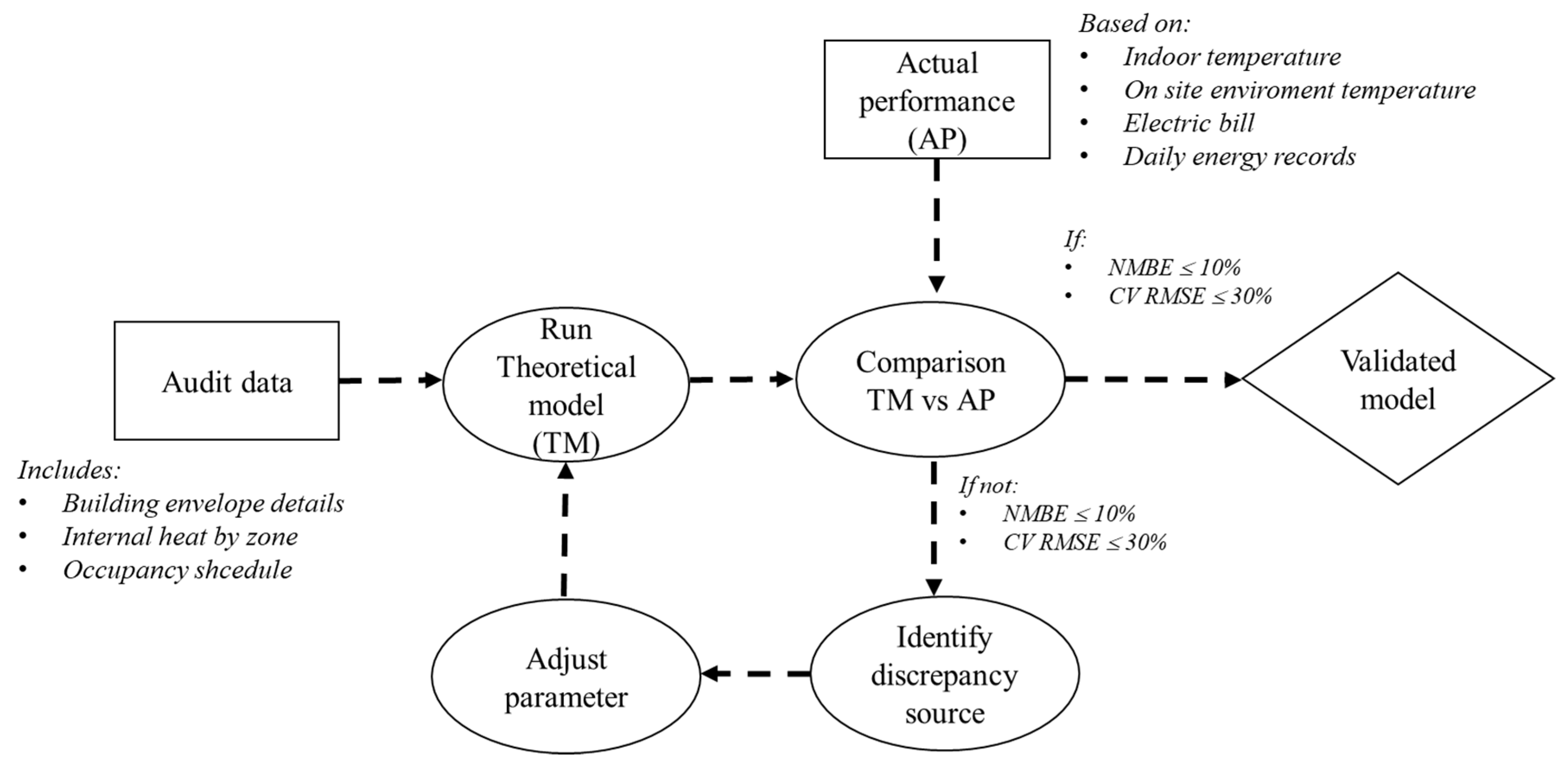
Figure 1. Framework of model validation (based on Hwa Cho and Sook Kim evaluation and American Society of Heating, Refrigerating and Air-Conditioning Engineers (ASHRAE) 14–2002 whole building calibrated approach).
Climate 07 00096 g001
Figure 2. Case study #1 (left) and case study #2 (right).
Climate 07 00096 g002
Figure 3. Average temperature of the year based on the typical meteorological year (TMY) file.
Climate 07 00096 g003
Figure 4. Graphical comparison between macro-environment (est. temp. °C) and micro-environment (in situ temp. °C) data in a week period. Above, Case 1; below, Case 2.
Climate 07 00096 g004
Figure 5. Graphical temperature and relative humidity comparison between actual and simulated data in each zone for Case 1.
Climate 07 00096 g005
Figure 6. Graphical temperature and relative humidity comparison between actual and simulated data in each zone for Case 2.
Climate 07 00096 g006
Figure 7. Electric consumption comparison in three levels: iteration 1, optimized iteration and actual energy reading.
Climate 07 00096 g007
Table 1. Nomenclature.
UHIUrban Heat Island
NAMANational Appropiate Mitigation Actions
EEREnergy Efficiency Ratio
NMBENominal Mean Bias Error
CV(RMSE) Coefficient of Variation of the Root Mean Square Error
ASHRAEAmerican Society of Heating, Refrigerating and Air-Conditioning Engineers
U-valueThermal Transmittance
Table 2. Design properties of each case of study.
Case 1Case 2
OrientationNortheastSouthwest
Total Ocupancy22
Area (m²)35.4542.5
ZonesLiving room/dinnerKitchen/dinner
Air conditioning Capacity kWKitchenBathroom
BathroomBedroom(storage)
BedroomMain bedroom
1.851.30
Energy efficiency ratio4.103.52
Table 3. Thermal envelope characteristics of each case studies.
Envelope elementCharacteristicsU-value (W/m²K) Case 1Case 2
Floor100 mm concrete slab 4.73YESYES
External/Inter-nal walls15mm exterior mortar, 150 mm concrete hollow block, 15 mm interior mortar2.66YESYES
Roof30mm concrete slab, 150 mm joist and concrete hollow brick, 15 mm interior mortar3.377YESYES
GlazingAbsorbent green 6 mm 5.808YESNO
Absorbent grey 6 mm 5.812NOYES
Window awning1.5 mm galvanized steel sheet8.33YESNO
Table 4. Preliminary analysis run simulation in both bedrooms from February to April, 2019, expressed as actual data (A) and simulated data (S).
TEMPERATURERELATIVE HUMIDITYENERGY CONSUMPTION kW
Mean A. °CMean S. °CNMBE%CV RMSE%Mean A. %Mean S. %NMBE%CV RMSE%APTM% ERROR
Case 128.6326.666.8910.8563.1365.29−3.4320.58711.70754.39−5.99
Case 225.7427.12−5.3610.4853.1464.41−21.2033.66202.60541.41−167.18
Table 5. Comparison between macro-environment data and micro-environment data.
Temperature °CRelative Humidity %
MIN. WEEKMAX. WEEKMEANMIN. WEEKMAX. WEEKMEAN
Case 1Macro- environment27.4032.3029.5467.0088.0078.65
Micro-environment26.7737.5430.1655.0185.9573.46
Case 2Macro- environment25.1033.7029.5550.0092.0073.98
Micro-environment25.3140.6731.0336.8985.1065.91
Table 6. Final comparison of level of compliance through checked uncertainty parameters between first iteration (ITER. 1), and optimized iteration (ITER. Op.)
TemperatureRelative Humidity
MEAN °CNMBE%CV (RMSE)%MEAN
%
NMBE%CV
(RMSE) %
Case 1BedroomITER. 10.2526.1116.0318.170.4160.857.2613.25
ITER. Op. 0.3728.297.1016.720.6866.52−1.8811.27
Living roomITER. 10.6728.4112.5712.970.3674.86−6.7910.70
ITER. Op.0.6831.760.682.620.6465.855.967.44
Case 2Main BedroomITER. 10.0929.35−5.0113.770.0663.86−29.5838.51
ITER. Op.0.3828.09−0.7411.010.0569.20−35.0140.49
Dinner/ kitchenITER. 10.5431.165.736.950.4064.27−9.5514.72
ITER. Op.0.6232.940.023.420.4370.58−8.9413.24
Bedroom (storage)ITER. 10.4730.277.928.700.4373.14−4.869.79
ITER. Op.0.5130.806.076.870.4468.970.886.39