Lagrangian Drifter to Identify Ocean Eddy Characteristics


Abstract
1. Introduction
2. Eddy Characteristics Identified at Each Data Point of an Individual RAFOS Float
3. Statistics of Eddy Characteristic Parameters
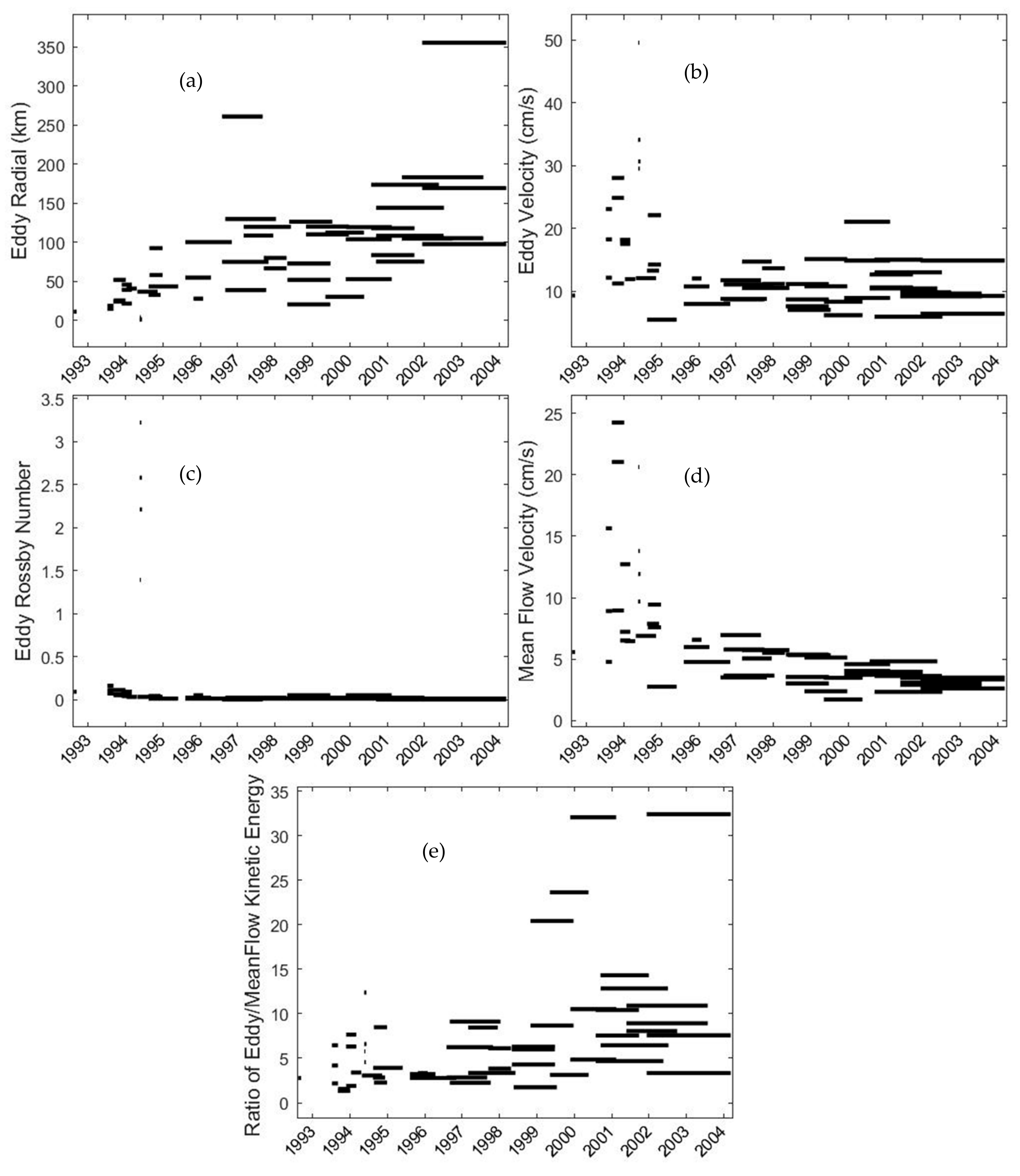
4. Temporal Variability of Eddy Characteristic Parameters
5. Conclusions
Author Contributions
Funding
Acknowledgments
Conflicts of Interest
References
- Chu, P.C. Steepest ascent low/non-low frequency ratio in empirical mode decomposition to separate deterministic and stochastic velocities from a single Lagrangian drifter. J. Geophys. Res. Oceans 2018, 123, 1708–1721. [Google Scholar] [CrossRef]
- Ivanov, L.M.; Chu, P.C. Estimation of turbulent diffusion coefficients from decomposition of Lagragian trajectories. Ocean Model. 2019, 137, 114–131. [Google Scholar] [CrossRef]
- Bauer, S.; Swenson, M.S.; Griffa, A.; Mariano, A.J.; Owens, K. Eddy-mean decomposition and eddy-diffusivity estimates in the tropical Pacific Ocean. J. Geophys. Res. Oceans 1998, 103, 30855–30871. [Google Scholar] [CrossRef]
- Galanis, G.N.; Louka, P.; Katsafados, P.; Pytharoulis, I. Applications of Kalman filters based on non-linear functions to numerical weather predictions. Ann. Geophys. 2006, 24, 2451–2460. [Google Scholar] [CrossRef]
- Lozano, C.J.; Robinson, A.R.; Arrango, H.G.; Gangopadhyay, A.; Sloan, Q.; Haley, P.J.; Anderson, L.; Leslie, W. An interdisciplinary ocean prediction system: Assimilation strategies and structured data models. In Modern Approaches to Data Assimilation in Ocean Modeling; Elsevier Oceanography Series; Malanotte-Rizzoli, P., Ed.; Elsevier: Amsterdam, The Netherlands, 1996; Volume 61, pp. 413–452. [Google Scholar]
- Chu, P.C.; Ivanov, L.M.; Korzhova, T.P.; Margolina, T.M.; Melnichenko, O.M. Analysis of sparse and noisy ocean current data using flow decomposition. Part 1: Theory. J. Atmos. Ocean. Technol. 2003, 20, 478–491. [Google Scholar] [CrossRef]
- Chu, P.C.; Ivanov, L.M.; Korzhova, T.P.; Margolina, T.M.; Melnichenko, O.M. Analysis of sparse and noisy ocean current data using flow decomposition. Part 2: Application to Eulerian and Lagrangian data. J. Atmos. Ocean. Technol. 2003, 20, 492–512. [Google Scholar] [CrossRef]
- Chu, P.C.; Fan, C.W. Accuracy progressive calculation of Lagrangian trajectory from gridded velocity field. J. Atmos. Ocean. Technol. 2014, 31, 1615–1627. [Google Scholar] [CrossRef]
- Huang, N.; Shen, Z.; Long, S.R.; Wu, M.C.; Smith, H.H.; Zheng, Q.; Yen, N.; Tung, C.C.; Liu, H.H. The empirical mode decomposition and the Hilbert spectrum for nonlinear and non-stationary time series analysis. Proc. R. Soc. Lond. 1998, 454, 903–995. [Google Scholar] [CrossRef]
- Chu, P.C.; Fan, C.W.; Huang, N. Compact empirical mode decomposition—An algorithm to reduce mode mixing, end effect, and detrend uncertainty. Adv. Adapt. Data Anal. 2012, 4, 1250017. [Google Scholar] [CrossRef]
- Chu, P.C.; Fan, C.W.; Huang, N. Derivative-optimized empirical mode decomposition for the Hilbert-Huang transform. J. Comput. Appl. Math. 2014, 259, 57–64. [Google Scholar] [CrossRef]
- Qiao, F.L.; Yuan, Y.L.; Deng, J.; Dai, D.J.; Song, Z.Y. Wave-turbulence interaction-induced vertical mixing and its effects in ocean and climate models. Philos. Trans. R. Soc. A 2016, 374, 20150201. [Google Scholar] [CrossRef] [PubMed]
- Collins, C.A.; Ivanov, L.M.; Melnichenko, O.B.; Gartfield, N. California Undercurrent variability and eddy transport estimated from RAFOS float observations. J. Geophys. Res. Oceans 2004, 109. [Google Scholar] [CrossRef]
- Collins, C.A.; Margolina, T.; Rago, T.A.; Ivanov, L.M. Looping RAFOS floats in the California Current System. Deep Sea Res. Part II Top Stud. Oceanogr. 2013, 85, 42–61. [Google Scholar] [CrossRef]
- Naval Postgraduate School RAFOS Float Data. Available online: https://www.oc.nps.edu/npsRAFOS/HTMLS/inventory_index.html (accessed on 23 November 2019).


| Float | Buoy Days | dbar | # C | # AC | Float | Buoy Days | dbar | # C | # AC |
|---|---|---|---|---|---|---|---|---|---|
| N002 * | 8/12–9/11/92 | 350 | 1 | 0 | N050 * | 8/29/96–1/9/98 | 275 | 3 | 2 |
| N003 * | 8/12–9/11/92 | 350 | 3 | 1 | N051 | 2/25/97–7/8/98 | 275 | 2 | 3 |
| N004 * | 7/07–9/05/93 | 350 | 1 | 3 | N053 * | 9/11/97–8/22/98 | 275 | 4 | 2 |
| N005 | 9/03/93–1/01/94 | 350 | 3 | 4 | N055 * | 9/11/97–8/22/98 | 275 | 1 | 1 |
| N006 | 11/20/93–5/02/94 | 350 | 0 | 1 | N062 * | 4/29/98–6/25/99 | 275 | 3 | 2 |
| N007 | 7/07–9/05/93 | 350 | 2 | 7 | N063 * | 5/17/98–7/12/99 | 275 | 0 | 2 |
| N008 | 9/3–12/30/93 | 350 | 3 | 4 | N064 * | 4/29/98–6/25/99 | 275 | 8 | 8 |
| N010 * | 9/3/93–1/1/04 | 350 | 2 | 2 | N065 * | 4/29/98–6/24/99 | 275 | 6 | 4 |
| N011 | 11/20/93–3/2/94 | 350 | 0 | 6 | N066 | 10/27/98–12/23/99 | 275 | 1 | 2 |
| N013 | 11/20/93–3/2/94 | 350 | 0 | 4 | N067 | 10/27/98–12/23/99 | 275 | 2 | 2 |
| N014 | 1/11–4/23/94 | 350 | 1 | 2 | N069 | 5/5/99–5/18/00 | 275 | 2 | 3 |
| N019 | 4/25–11/11/94 | 275 | 2 | 3 | N071 * | 5/5/99–5/18/00 | 275 | 4 | 6 |
| N021 * | 5/19–6/10/94 | 275 | 12 | 16 | N072 | 11/21/99–2/12/01 | 275 | 5 | 3 |
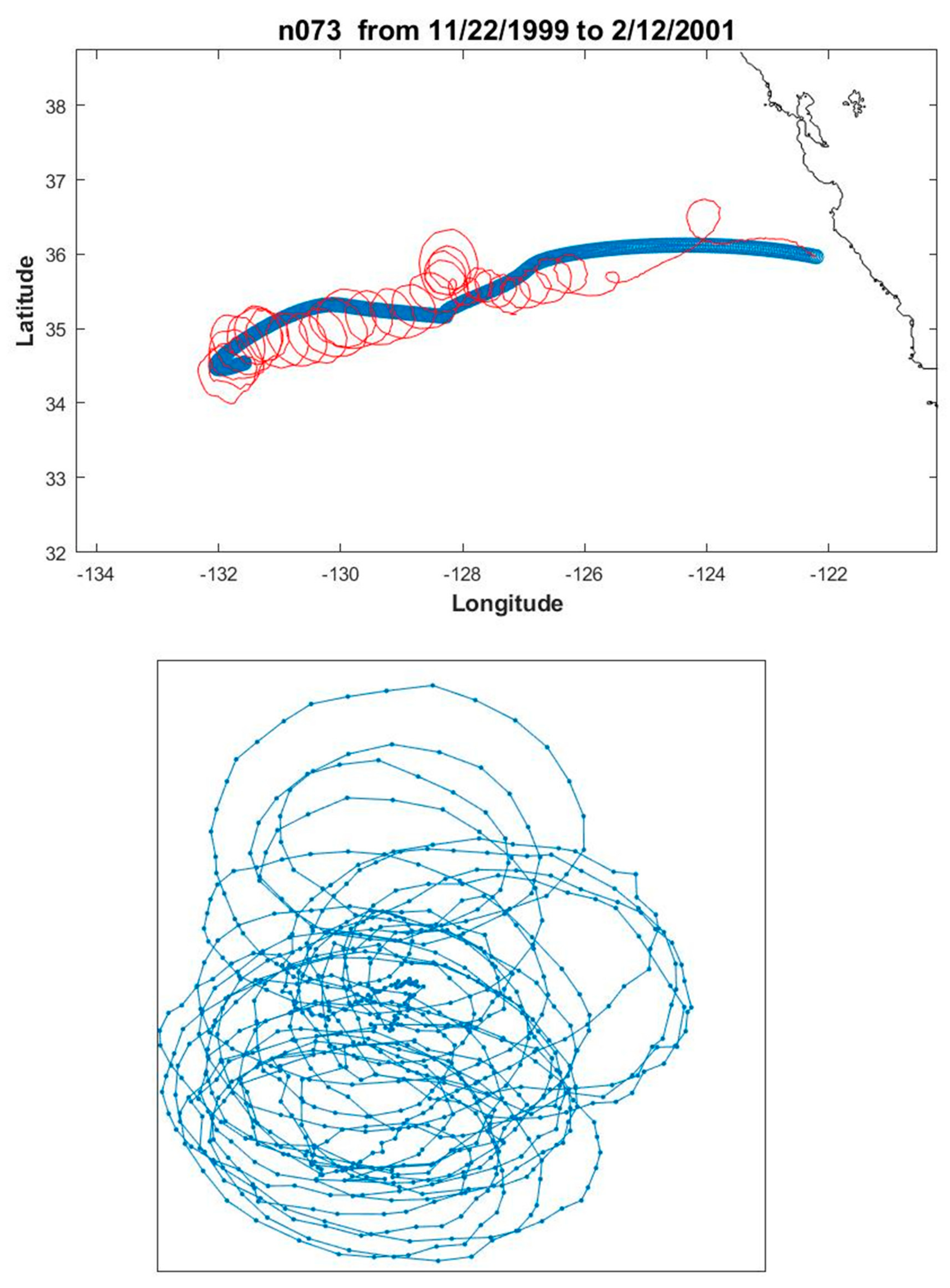
| N022 * | 5/19–6/10/94 | 275 | 12 | 15 | N073 | 11/21/99–2/12/01 | 275 | 4 | 19 |
| N024 * | 5/17–6/9/94 | 275 | 13 | 27 | N075 | 11/21/99–2/12/01 | 275 | 3 | 4 |
| N026 | 8/22–12/30/94 | 290 | 3 | 5 | N080 * | 7/26/00–9/23/01 | 275 | 2 | 2 |
| N028 | 8/12–12/19/94 | 350 | 2 | 4 | N081 * | 7/26/00–5/22/02 | 275 | 3 | 2 |
| N029 * | 10/25/95–6/28/96 | 300 | 2 | 2 | N082 * | 7/26/00–9/24/01 | 275 | 6 | 2 |
| N030 * | 5/18–6/10/94 | 275 | 14 | 19 | N083 | 9/11/00–12/29/01 | 275 | 4 | 7 |
| N031 | 8/22–12/30/94 | 290 | 0 | 4 | N084 * | 9/11/00–7/9/02 | 275 | 1 | 2 |
| N032 * | 8/7/95–10/6/96 | 300 | 3 | 1 | N085 | 9/11/00–7/9/02 | 275 | 7 | 2 |
| N033 | 8/12/94–5/10/95 | 350 | 4 | 2 | N087 * | 5/20/01–11/6/02 | 275 | 2 | 2 |
| N035 * | 8/7/95–11/5/96 | 300 | 1 | 3 | N088 | 5/20/01–7/28/03 | 275 | 4 | 8 |
| N039 * | 7/29/96–12/10/97 | 275 | 2 | 4 | N089 | 5/20/01–7/28/03 | 275 | 4 | 1 |
| N041 | 7/29/96–11/17/97 | 275 | 1 | 2 | N090 | 12/6/01–3/9/04 | 275 | 4 | 4 |
| N043 | 2/25–12/13/97 | 275 | 0 | 4 | N091 | 12/5/01–3/9/04 | 275 | 3 | 7 |
| N048 | 7/29/96–9/19/97 | 275 | 5 | 4 | N092 * | 12/5/01–3/9/04 | 275 | 6 | 2 |
| Total | 186 | 253 |
| Parameter | Mean | Min | Max | Standard Deviation | Skewness | Kurtosis |
|---|---|---|---|---|---|---|
| (km) | 18.37 | 1.12 | 102.21 | 21.33 | 2.31 | 8.50 |
| (cm/s) | 11.98 | 2.72 | 44.17 | 8.65 | 1.74 | 5.82 |
| (cm/s) | 10.04 | 4.19 | 31.59 | 5.39 | 2.38 | 8.96 |
| 0.35 | 0.01 | 3.99 | 0.86 | 3.34 | 12.90 | |
| 1.78 | 0.13 | 11.19 | 2.00 | 2.79 | 12.00 |
© 2019 by the authors. Licensee MDPI, Basel, Switzerland. This article is an open access article distributed under the terms and conditions of the Creative Commons Attribution (CC BY) license (http://creativecommons.org/licenses/by/4.0/).
Share and Cite
Chu, P.C.; Fan, C. Lagrangian Drifter to Identify Ocean Eddy Characteristics. Climate 2019, 7, 137. https://doi.org/10.3390/cli7120137
Chu PC, Fan C. Lagrangian Drifter to Identify Ocean Eddy Characteristics. Climate. 2019; 7(12):137. https://doi.org/10.3390/cli7120137
Chicago/Turabian StyleChu, Peter C., and Chenwu Fan. 2019. "Lagrangian Drifter to Identify Ocean Eddy Characteristics" Climate 7, no. 12: 137. https://doi.org/10.3390/cli7120137
APA StyleChu, P. C., & Fan, C. (2019). Lagrangian Drifter to Identify Ocean Eddy Characteristics. Climate, 7(12), 137. https://doi.org/10.3390/cli7120137