Deciphering Active Wildfires in the Southwestern USA Using Topological Data Analysis

Abstract
1. Introduction
2. Data and Methods
2.1. Data
2.2. Topological Data Analysis
3. Results
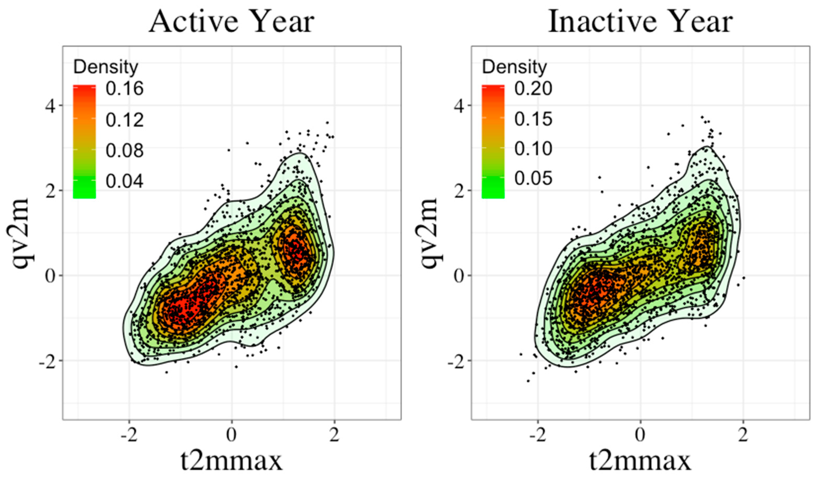
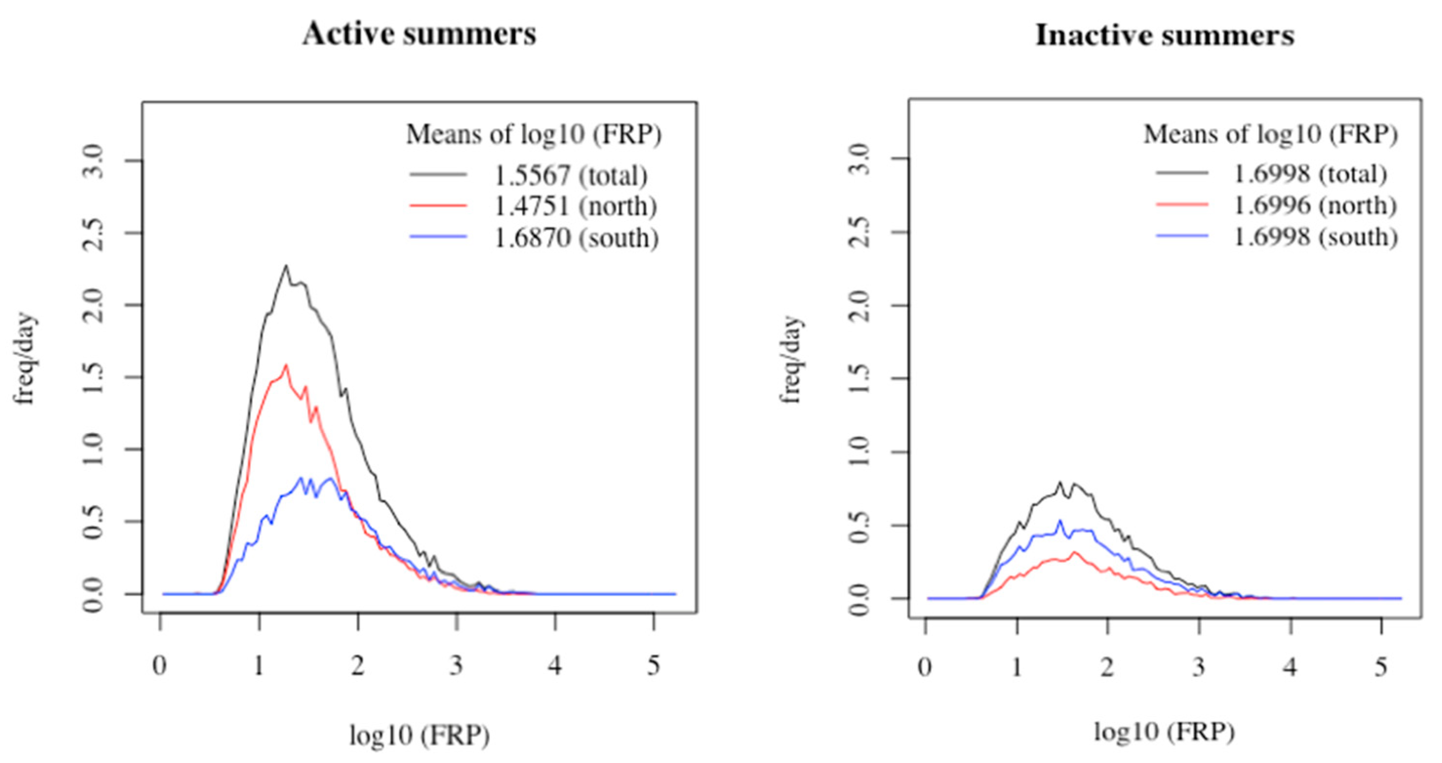
3.1. Climatology
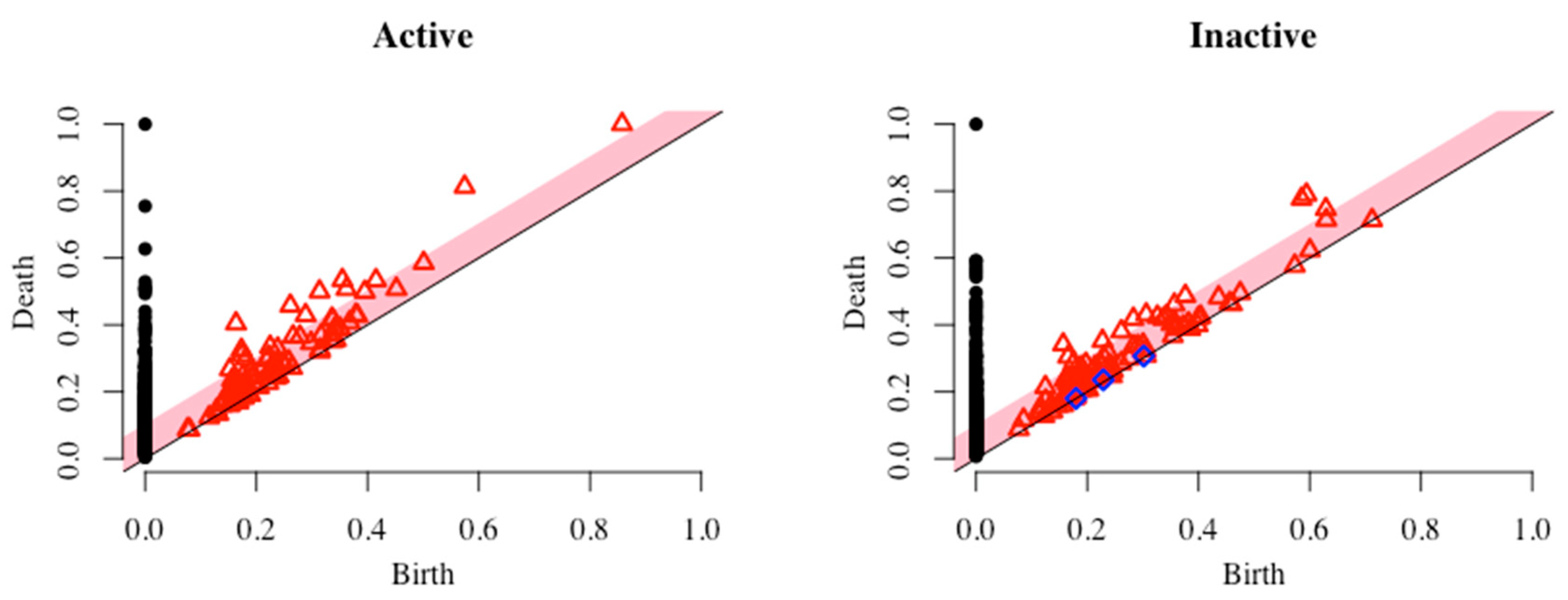
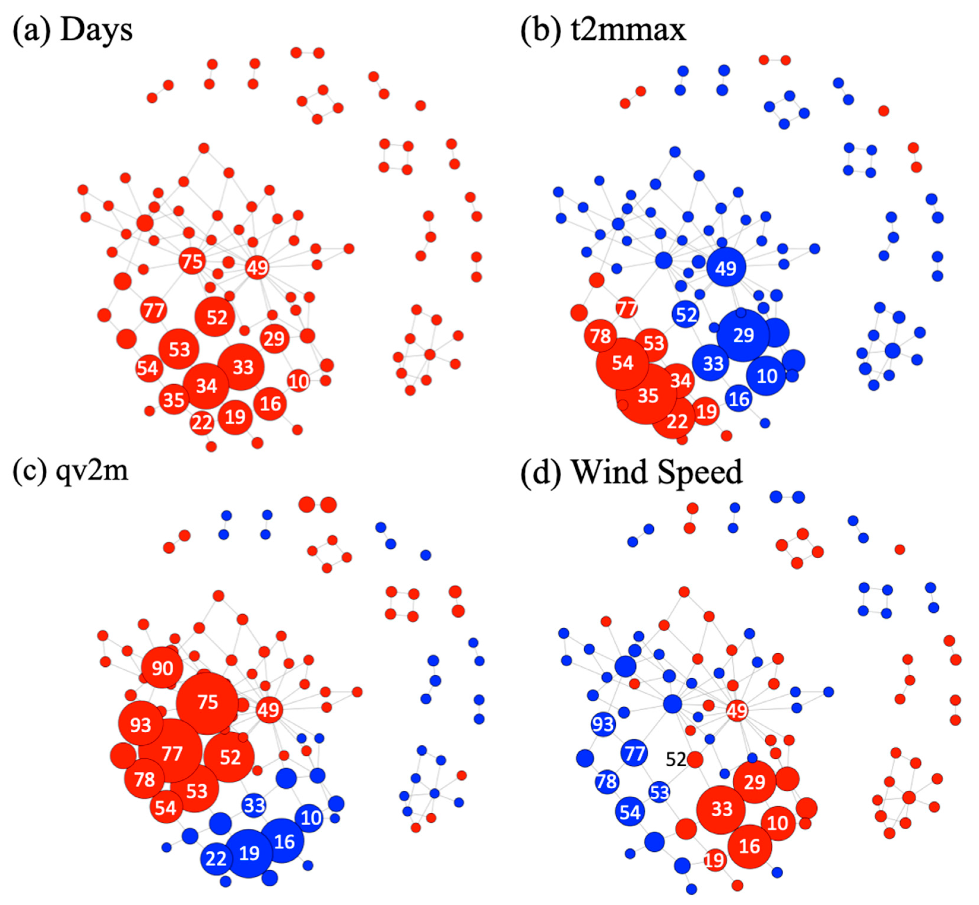
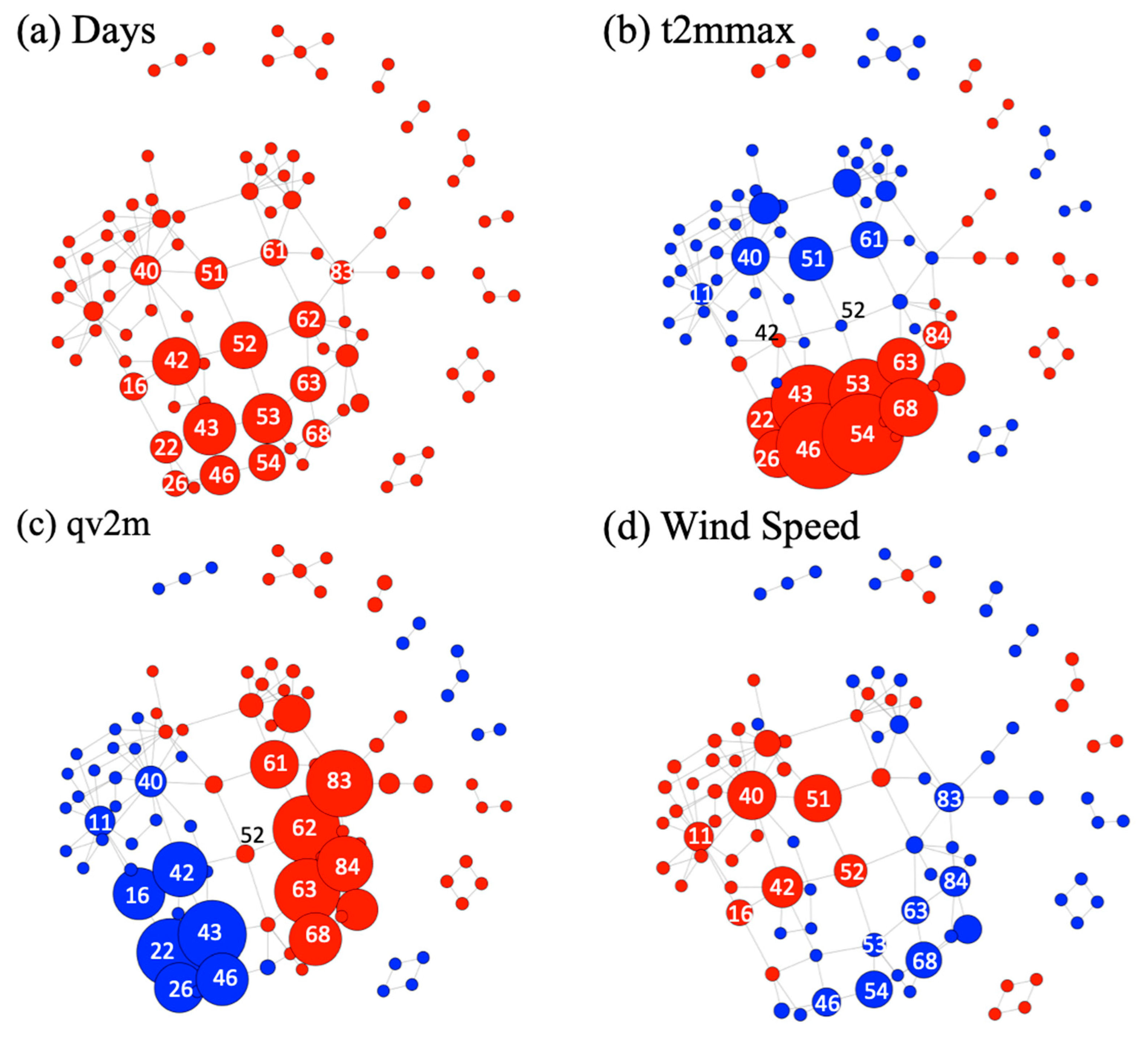
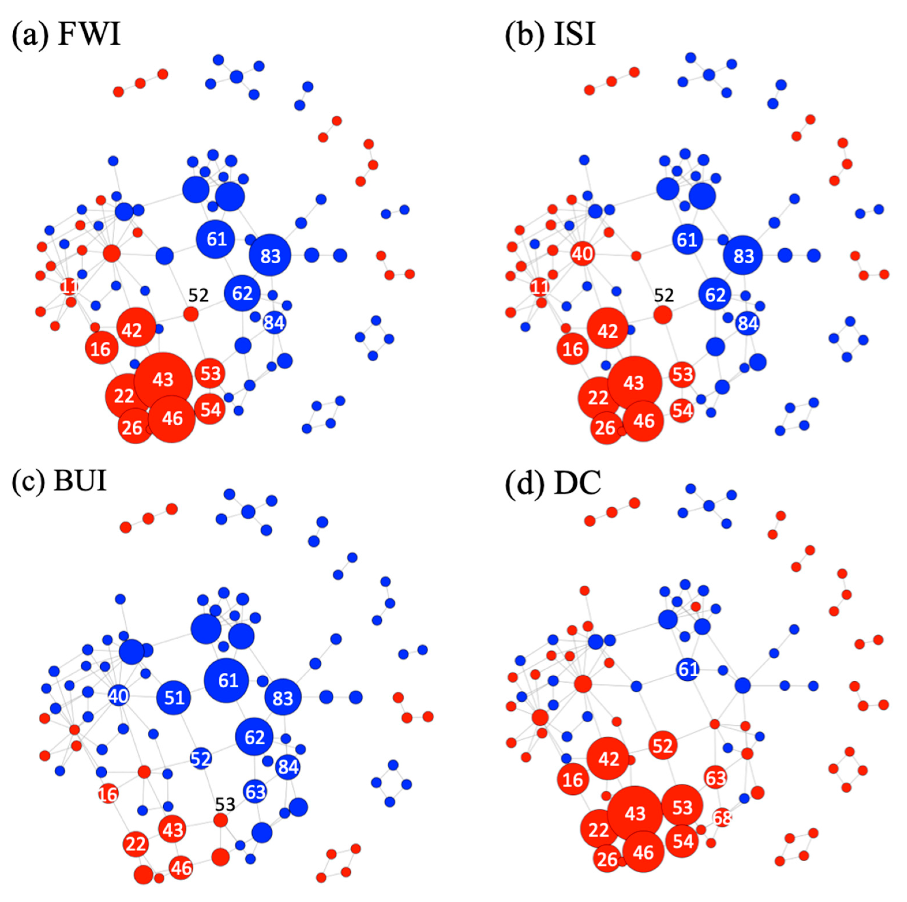
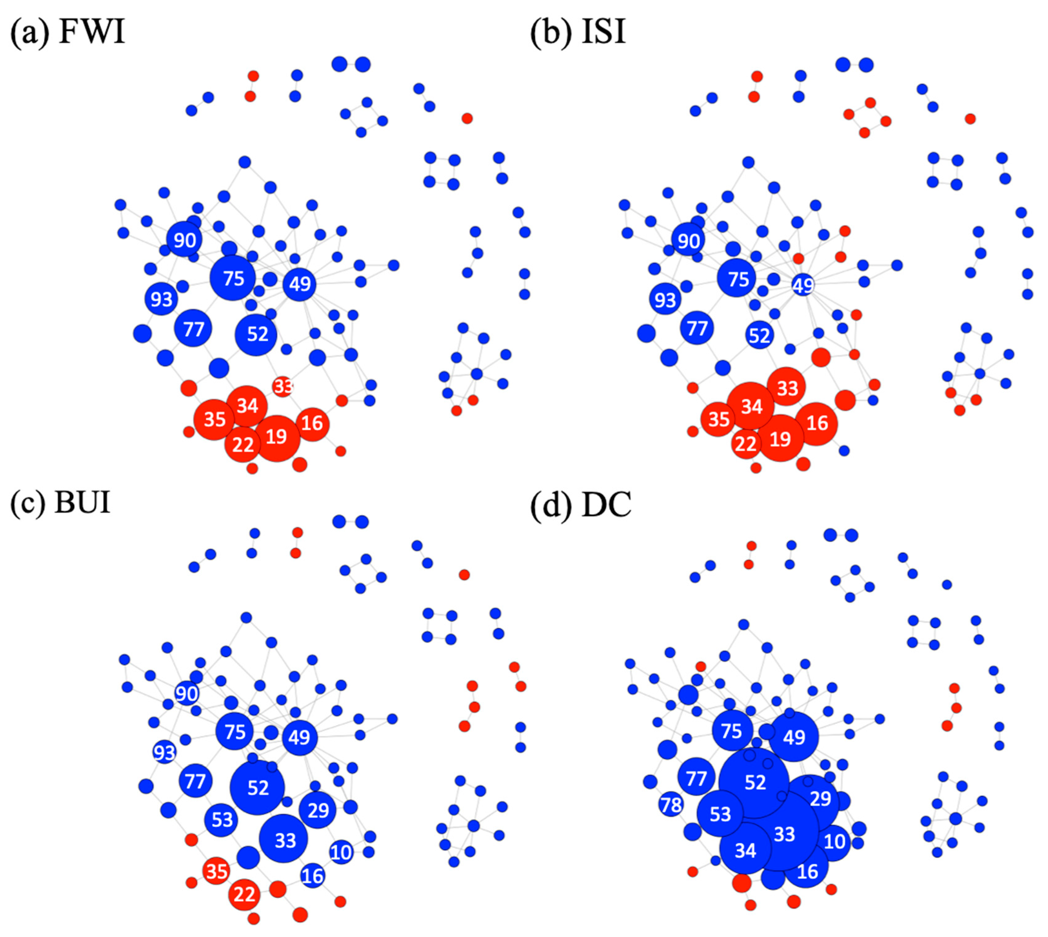
3.2. Topological Data Analysis
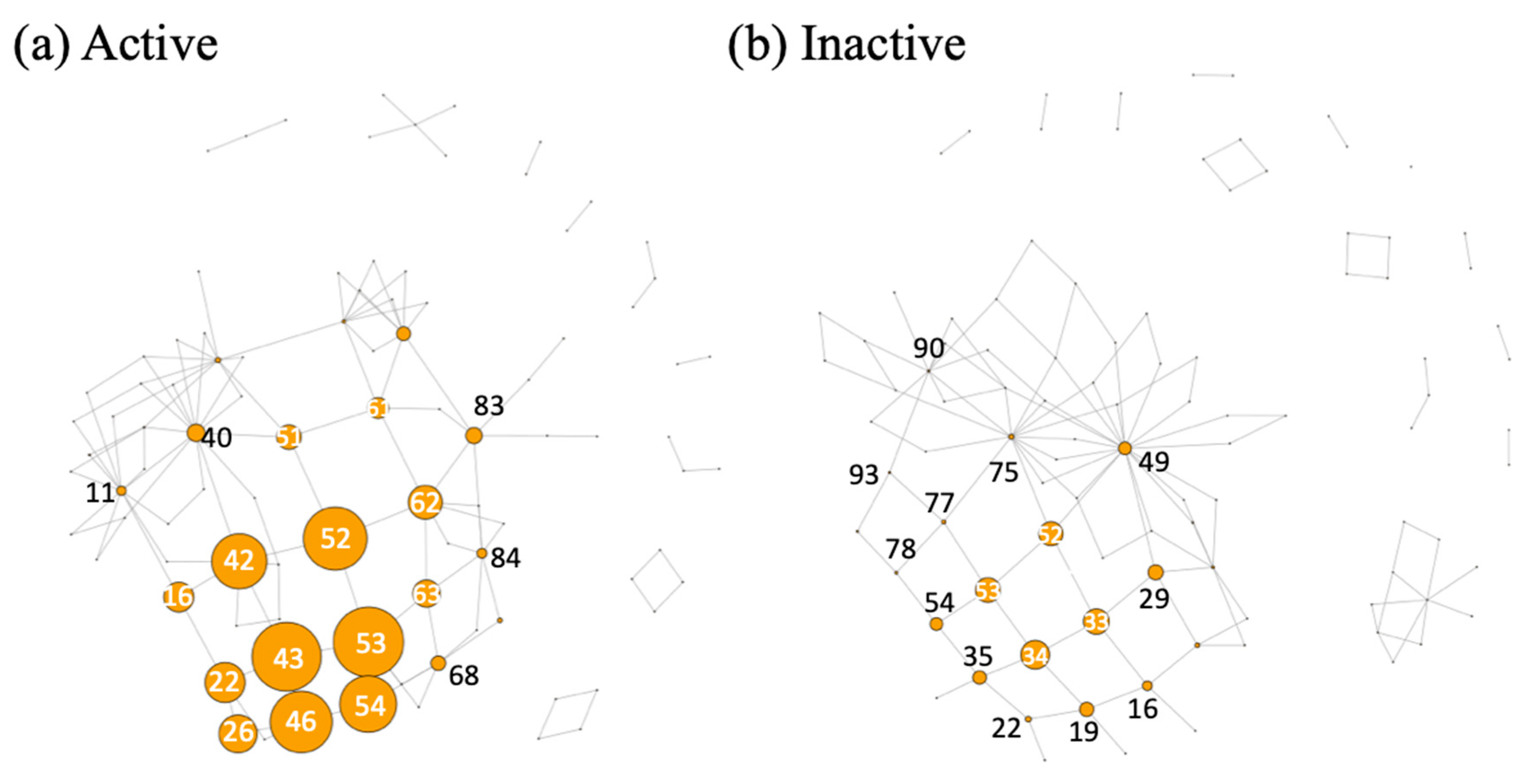
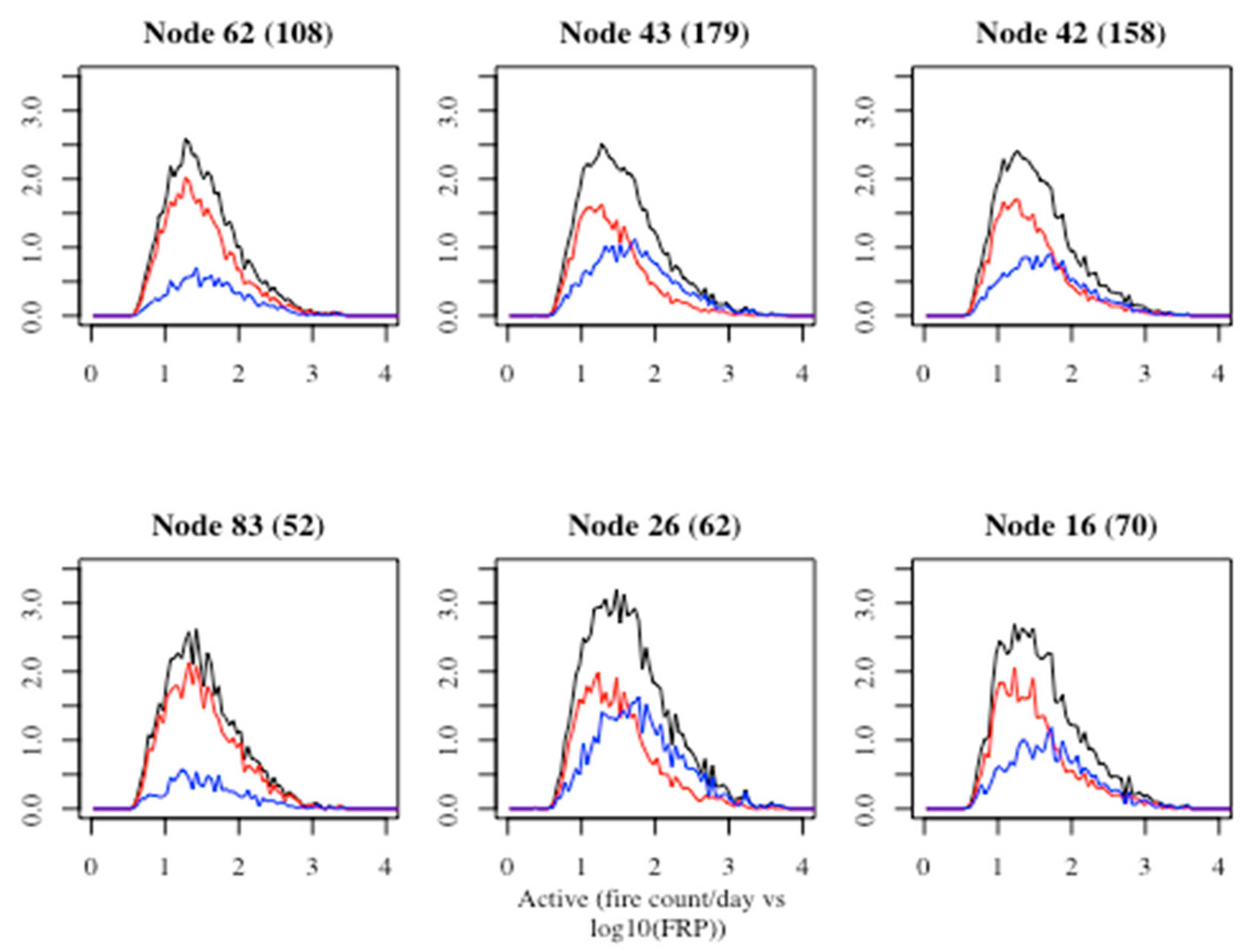
3.3. TDAMapper
4. Conclusions
Author Contributions
Funding
Acknowledgments
Conflicts of Interest
References
- Smith, A.B.; Katz, R.W. US billion-dollar weather and climate disasters: Data sources, trends, accuracy and biases. Nat. Hazards 2013, 67, 387–410. [Google Scholar] [CrossRef]
- Malmsheimer, R.W.; Bowyer, J.L.; Fried, J.S.; Gee, E.; Izlar, R.L.; Miner, R.A.; Munn, I.A.; Oneil, E.; Stewart, W.C. Managing Forests Because Carbon Matters: Integrating Energy, Products, and Land Management. Policy. J. For. 2011, 109, S5–S48. [Google Scholar]
- Verdin, K.L.; Dupree, J.A.; Elliott, J.G. Probability and Volume of Potential Postwildfire Debris Flows in the 2012 High Park Burn Area near Fort Collins, Colorado. In Open-File Report; U.S. Geological Survey: Reston, VA, USA, 2012. [Google Scholar]
- NOAA National Centers for Environmental Information (NCEI) U.S. Billion-Dollar Weather and Climate Disasters. 2019. Available online: https://www.ncdc.noaa.gov/billions/ (accessed on 15 November 2016).
- Cayan, D.R.; Das, T.; Pierce, D.W.; Barnett, T.P.; Tyree, M.; Gershunov, A. Future dryness in the southwest US and the hydrology of the early 21st century drought. Proc. Natl. Acad. Sci. USA 2010, 107, 21271–21276. [Google Scholar] [CrossRef] [PubMed]
- Westerling, A.L.; Hidalgo, H.G.; Cayan, D.R.; Swetnam, T.W. Warming and Earlier Spring Increase Western U.S. Forest Wildfire Activity. Science 2006, 313, 940. [Google Scholar] [CrossRef] [PubMed]
- Crockett, J.L.; Westerling, A.L. Greater temperature and precipitation extremes intensify western US droughts, wildfire severity, and Sierra Nevada tree mortality. J. Clim. 2018, 31, 341–354. [Google Scholar] [CrossRef]
- Haines, D.A. A lower atmospheric severity index for wildland fire. Natl. Weather. Dig. 1988, 13, 23–27. [Google Scholar]
- Van Wagner, C.E. Development and Structure of the Canadian Forest Fire Weather Index System; Canadian Forestry Service Ottawa: Ottawa, ON, Canada, 1987. [Google Scholar]
- McEvoy, D.J.; Hobbins, M.; Brown, T.J.; VanderMolen, K.; Wall, T.; Huntington, J.L.; Svoboda, M. Establishing relationships between drought indices and wildfire danger outputs: A test case for the California-Nevada drought early warning system. Climate 2019, 7, 52. [Google Scholar] [CrossRef]
- Balch, J.K.; Bradley, B.A.; Abatzoglou, J.T.; Nagy, R.C.; Fusco, E.J.; Mahood, A.L. Human-started wildfires expand the fire niche across the United States. Proc. Natl Acad. Sci. USA 2017, 114, 2946–2951. [Google Scholar] [CrossRef] [PubMed]
- Justice, C.O.; Giglio, L.; Korontzi, S.; Owens, J.; Morisette, J.; Roy, D.; Descloitres, J.; Alleaume, S.; Petitcolin, F.; Kaufman, Y.J. The MODIS fire products. Remote Sens. Environ. 2002, 83, 244–262. [Google Scholar] [CrossRef]
- Ichoku, C.; Kaufman, Y.J. A method to derive smoke emission rates from MODIS fire radiative energy measurements. IEEE Trans. Geosci. Remote Sens. 2005, 43, 2636–2649. [Google Scholar] [CrossRef]
- Giglio, L.; Schroeder, W.; Hall, J.V.; Justice, C.O. MODIS Collection 6 Active Fire Product User’s Guide. Revision B; University of Maryland: College Park, MD, USA, 2018; p. 64. [Google Scholar]
- Charzal, F.; de Solva, V.; Oudot, S. Persistence stability for geometric complexes. Geom. Dedicata. 2014, 173, 193–214. [Google Scholar] [CrossRef]
- Bubenik, P. Statistical topological data analysis using persistence landscapes. J. Mach. Learn. Res. 2015, 16, 77–102. [Google Scholar]
- Singh, G.; Memoli, F.; Carlsson, G. Topological methods for the analysis of high dimensional data sets and 3D object recognition. Eurogr. Symp. Point-Based Graph. 2007. [Google Scholar] [CrossRef]
- Giansiracusa, N.; Giansiracusa, R.; Moon, C. Persistent homology machine learning for fingerprint classification. arXiv 2017, arXiv:1711.09158v1. [Google Scholar]
- Gidea, M.; Katz, Y. Topological data analysis of financial time series: Landscapes of crashes. Physica A 2018, 491, 820–834. [Google Scholar] [CrossRef]
- Nicolau, M.; Levine, A.J.; Carlsson, G. Topology based data analysis identifies a subgroup of breast cancers with a unique mutational profile and excellent survival. Proc. Natl. Acad. Sci. USA 2011, 108, 7265–7270. [Google Scholar] [CrossRef] [PubMed]
- Lum, P.Y.; Singh, G.; Lehman, A.; Ishkanov, T.; Vejdemo-Johansson, M.; Alagappan, M.; Carlsson, J.; Carlsson, G. Extracting insights from the shape of complex data using topology. Sci. Rep. 2013, 3, 1236. [Google Scholar] [CrossRef]
- Muszynski, G.; Kashinath, K.; Kurlin, V.; Wehner, M.; Prabhat. Topological data analysis and machine learning for recognizing atmospheric river patterns in large climate datasets. Geosci. Model Dev. 2019, 12, 613–628. [Google Scholar] [CrossRef]
- Westerling, A.L.; Gershunov, A.; Brown, T.J.; Cayan, D.R.; Dettinger, M.D. Climate and wildfire in the western United States. Bull. Am. Meteorol. Soc. 2003, 84, 595–604. [Google Scholar] [CrossRef]


| Active Summers | Inactive Summers | ||
|---|---|---|---|
| Year | Burned area (acre) | Year | Burned area (acre) |
| 2008 | 336,000 | 2010 | 19,107 |
| 2016 | 227,503 | 1997 | 23,489 |
| 2006 | 164,574 | 2007 | 26,000 |
| 2015 | 130,537 | 2011 | 31,232 |
| 1999 | 124,681 | 2005 | 49,539 |
© 2019 by the authors. Licensee MDPI, Basel, Switzerland. This article is an open access article distributed under the terms and conditions of the Creative Commons Attribution (CC BY) license (http://creativecommons.org/licenses/by/4.0/).
Share and Cite
Kim, H.; Vogel, C. Deciphering Active Wildfires in the Southwestern USA Using Topological Data Analysis. Climate 2019, 7, 135. https://doi.org/10.3390/cli7120135
Kim H, Vogel C. Deciphering Active Wildfires in the Southwestern USA Using Topological Data Analysis. Climate. 2019; 7(12):135. https://doi.org/10.3390/cli7120135
Chicago/Turabian StyleKim, Hannah, and Christian Vogel. 2019. "Deciphering Active Wildfires in the Southwestern USA Using Topological Data Analysis" Climate 7, no. 12: 135. https://doi.org/10.3390/cli7120135
APA StyleKim, H., & Vogel, C. (2019). Deciphering Active Wildfires in the Southwestern USA Using Topological Data Analysis. Climate, 7(12), 135. https://doi.org/10.3390/cli7120135