Article

Multi-Model Forecasts of Very-Large Fire Occurences during the End of the 21st Century

1
College of the Environment Special Programs, Quantitative Ecology & Resource Management (QERM), University of Washington, Seattle, WA 98195, USA
2
Pacific Wildland Fire Sciences Laboratory, U.S. Forest Service, 400 N. 34th St #201, Seattle, WA 98103, USA
3
Department of Statistics and School of Aquatic and Fishery Sciences, University of Washington, Seattle, WA 98195, USA
4
Daniel J. Evans School of Public Policy and Governance, University of Washington, Seattle, WA 98195, USA
5
Pacific Wildland Fire Sciences Laboratory, School of Environmental and Forest Sciences, University of Washington, Seattle, WA 98195, USA
*
Author to whom correspondence should be addressed.
Climate 2018, 6(4), 100; https://doi.org/10.3390/cli6040100
Submission received: 9 November 2018 / Revised: 12 December 2018 / Accepted: 13 December 2018 / Published: 19 December 2018
(This article belongs to the Special Issue Climate Variability and Change in the 21th Century)

Abstract

:
Climate change is anticipated to influence future wildfire activity in complicated, and potentially unexpected ways. Specifically, the probability distribution of wildfire size may change so that incidents that were historically rare become more frequent. Given that fires in the upper tails of the size distribution are associated with serious economic, public health, and environmental impacts, it is important for decision-makers to plan for these anticipated changes. However, at least two kinds of structural uncertainties hinder reliable estimation of these quantities—those associated with the future climate and those associated with the impacts. In this paper, we incorporate these structural uncertainties into projections of very-large fire (VLF)—those in the upper 95th percentile of the regional size distribution—frequencies in the Continental United States during the last half of the 21st century by using Bayesian model averaging. Under both moderate and high carbon emission scenarios, large increases in VLF frequency are predicted, with larger increases typically observed under the highest carbon emission scenarios. We also report other changes to future wildfire characteristics such as large fire frequency, seasonality, and the conditional likelihood of very-large fire events.

1. Introduction

Although representing only a small fraction of the total number of fires, very-large fires (VLFs) are events often associated with dramatic economic, human health, and environmental risks that are unlike most other wildfires. The most salient and immediate economic impacts are suppression costs and property losses (Barrett 2018, [1]), which are often relatively large in VLFs compared to other smaller events (González-Cabán 1983 [2], Stephens et al., 2014 [3]). In addition to these direct costs, there is a suite of indirect economic impacts—such as damages from post-fire hazards, rehabilitation costs, lost tax and business revenue from community evacuations (Dale 2009 [4])—that are increasingly probable and costly in larger wildfires (Neary et al., 2003 [5], Peppin et al., 2011 [6], Beverly and Bothwell 2011 [7], Beverly et al., 2011 [8]). VLFs have the potential to burn large areas of vegetation and emit tremendous quantities of smoke within a short duration of time, which can adversely impact air quality for months at a time (Stephens et al., 2014 [3]), even at long distances from any active burning (Forster et al., 2001 [9], Val Martin et al., 2013 [10]). The large areas of active burning and sudden increase in air pollutants pose numerous risks to public health (Reid et al., 2016 [11]) and safety (Achtemeier 2009 [12], Stephens et al., 2014 [3]); and hospital admissions and treatment costs are expected to increase during VLFs (Moeltner et al., 2013 [13]). Although there are some ecological benefits of fire, VLFs have also been associated with significant, deleterious, and sometimes irreversible environmental changes. These include the production of environmental conditions conducive to the establishment of invasive species (Crawford et al., 2001 [14]), loss of ecosystem services (Rocca et al., 2014 [15]), and long-term modifications to forest structure (Haffey et al., 2018 [16]). Given the disproportionate costs VLFs pose to economic, social and environmental values, there is a broad need across disciplines, to better understand patterns and trends of their occurrence to mitigate future hazards. There is even greater urgency for this given that multiple lines of evidence suggest that VLF frequency has increased (Williams 2013 [17], Dennision et al., 2014 [18], Barbero et al., 2014 [19]) and will continue to increase into the future (Stavros et al., 2014 [20], Barbero et al., 2015 [21]). Still, there are several challenges to obtaining reliable predictions of future wildfire activity, many of which are related to various kinds of scientific unknowns or uncertainties. These uncertainties can come from many sources (Chen et al., 2018 [22]) and can be associated with a particular quantity of interest—what will the future frequency of very-large fire events be?—or associated with model structures—how are environmental conditions related to very-large fire frequency? The latter is referred to as model or structural uncertainties, which can have significant effects on the conclusions one draws from an analysis (Morgan et al., 1992 [23], Syphard et al., 2018 [24]). In the context of forecasting future wildfire activities, these structural uncertainties can arise from the selection of vegetation models (Sitch et al., 2008 [25], Syphard et al., 2018 [24]), assumed anthropogenic effects (Westerling et al., 2011 [26]), as well as greenhouse gas emmissions and their effects on the environment.
Structural uncertainties associated with the characteristics of the future environment are commonly accounted for in long-term climate impact studies through the use of multiple General Circulation Models (GCMs). Each GCM predicts climatological responses based on unique assumptions regarding chemical and physical interactions between a suite of factors including land, water, atmosphere, and the cryosphere. These models can be used to forecast future climate by forcing the models to observe historical atmospheric conditions and running the models forward using representative concentration pathways (RCPs) as plausible carbon emission scenarios. There are four future RCP scenarios, which are labeled RCP 8.5, RCP 6, RCP 4.5, and RCP 2.6; each assumes various levels of fossil fuel use and economic activity. The suffix labels correspond to the approximate 2100 radiative forcing levels. For instance, the high-emission (RCP 8.5) scenario corresponds to an approximate radiative forcing increase of 8.5 W/m2 by 2100 compared to pre-industrial conditions. Since the choice of GCM and RCP can be thought of as competing plausible models of the future environment, and the precise climatological response and quantities of greenhouse gases that will be emitted and sequestered prior to 2100 are unknown, it makes sense to interpret them as structural uncertainties (Taylor et al., 2012 [27]).
In addition to the structural uncertainty arising from relating greenhouse gas emission scenarios to climatological impacts, structural uncertainty further arises when relating climatological variables to an impact of interest. In the context of fire, these relationships could include weather patterns such as temperature, precipitation, atmospheric moisture, winds, and clouds. Identifying and describing the relationship between these variables and VLFs is an immensely complex and subjective process, as there can be many competing hypotheses. For instance, temperature controls landscape flammability, is associated with thunderstorm activity and by extension ignition frequency (Flannigan et al., 2009 [28]), mediates tree mortality through drought (Allen et al., 2010 [29]) and insect pests (Bentz et al., 2010 [30]), and influences the length of the snow-free season (Westerling 2016 [31]). Additionally, the timing and amount of precipitation can also influence wildfire behavior in parallel with temperature by controlling the availability of fine fuels (Meyn et al., 2007 [32]), fuel moisture (Flannigan et al., 2016 [33]), and distribution of flammable species (Bradley et al., 2016 [34]). Multiple weather variables may adequately measure a common phenomenon associated with wildfire risk, such as drought (Zargar et al., 2011 [35]), resulting in highly correlated covariates that when utilized in wildfire risk prediction, produce models with near-identical goodness-of-fit. Hence, although statistical models can be a useful tool for representing and identifying the relative importance of relationships between the environment and fire, they are still only approximations to reality. Confounding of unmeasured variables like vegetation management (Holsinger et al., 2016 [36]) may influence the predicted importance of some weather variables, which can make model selection challenging. In some cases, the same suite of covariates can be used to make predictions with multiple mathematical representations (Mallick and Gelfand 1994 [37]), presenting an additional level of uncertainty that is easily overlooked. Given the frequency with which we face structural uncertainties when modeling highly complex phenomena like wildfire, it is extremely risky to select any single model as an approximation of this phenomena, and a more robust approach should explore results from multiple models (Morgan et al., 1992 [23], Littel et al., 2011 [38]).
Bayesian model averaging is flexible and a commonly used method of accounting for structural uncertainties like these, lessening many of the risks of traditional model selection techniques and improving performance across a variety of metrics (Raftery and Zheng 2003 [39]). Within this framework, model weights, which are assumed to be uncertain, are used to combine covariates or predictions from multiple sources into a single probability distribution. The uncertainties in the model weights are represented using the posterior, which is a probability distribution representing the belief in the model parameters conditional on the observed data. While posteriors provide a natural framework for interpreting uncertainties, in practice, closed form expressions of the posterior are non-trivial and direct calculation is often impossible. Hence, simulation methods like Markov Chain Monte Carlo are typically used to generate samples from the distribution, which are in turn used to approximate the quantities that are of interest to the analyst (Fragoso et al., 2018 [40]). Computational barriers to Markov Chain Monte Carlo techniques have diminished greatly since they were first introduced, and a range of recently developed software options such as JAGS (Plummer 2003 [41]), Stan (Carpenter et al., 2017 [42]), and Integrated Nested Laplace Approximations (Rue et al., 2009 [43]) have facilitated the application of these methods in novel and previously infeasible contexts (Monnahan et al., 2017 [44]).
Hence, in this paper, we account for both kinds of structural uncertainty—uncertainty from the climate models and uncertainty from the choice of VLF models—using Bayesian model averaging to generate predictions of event frequency in the last half of the 21st century in the Continental United States. In Section 2, we present the methods used to produce robust predictions of future wildfire activity using GCMs and multiple fire occurrence models. In Section 3, the results of this analysis are available and demonstrate that increases in VLF activity should be expected in many regions in the Continental United States at the end of the century. In Section 4, we close the paper with a discussion of the implications of this analysis to decision-makers and researchers.

2. Methods

2.1. Fire Occurrence Data

Data from the Monitoring Trends in Burn Severity (MTBS) project [45], which describes individual fire size and severity based on changes in satellite imagery, are used to measure monthly fire occurrence. The original dataset included all detected fire events within the continental United States for the years 1984–2015 and is further filtered to remove all events 404 hectares or smaller, or that were non-wildfire. The filtered data are grouped into 18 regions with broadly similar climate and vegetation characteristics using a geospatial dataset of ecosystem divisions (Figure 1, Bailey 2016 [46]). For each region, two binary time series were constructed: one representing large fire (LF) occurrence, and another representing very-large fire (VLF) occurrence. The LF occurrence time series, X L F , t , reports “1” if at least 1 event of at least 404 hectares is recorded during that month; otherwise, it reports “0”. The VLF occurrence time series, X V L F , t , records “1” if at least 1 VLF—one that exceeds the 95th percentile of the region’s filtered MTBS burn area records (Table 1)—is recorded during that month and region; otherwise, it reports “0”. The Marine Division had one fire event and the Subtropical Regime Mountain had no VLF events during 1984–2005, and both were dropped from further consideration, yielding a total of 16 independent ecoregional analyses. All of the time series are split into a tuning dataset (1984–2005) and a training dataset (2006–2015).

2.2. Meteorological Covariates

Regional averages of gridded weather variables from the University of Idaho gridMET dataset [47] are used to calculate 12 weather predictors that will provide coarse scale environmental descriptions during each month between 1984–2015. Of these 12 weather predictors, four are measures of temperature; six are measures of moisture levels, and two measure wind characteristics. The four temperature metrics are based on monthly space-time averages of daily average temperature, which are calculated by dividing the sum of the daily maximum and minimum values by two (Weiss et al., 2005 [48]). The quantity hereafter referred to as seasonality measures intra-annual temperature variability by normalizing monthly temperature averages by the mean and standard deviation of all 360 measurements in the most recent 30 years of data (e.g., 1986–2015). The inter-annual temperature variability is captured with a quantity referred to as the departure from normal, which instead normalizes by the mean and standard deviation of 30 measurements in the most recent 30 years of data that correspond to same month as the raw measurement. The remaining temperature metrics are the rolling 12-month minimum and maximum temperature, which will record extreme temperature events that have potential for delayed impacts on wildfire activity. The six moisture level metrics are average specific humidity and precipitation totals over five time periods (1, 3, 6, 12 and 24-month time windows). In addition to a simple space-time average of wind speed at 10 m, the maximum daily space-time average each month was also included as a covariate of the fire occurrence probabilities.

2.3. Probability Estimation Trees

Two quantities are estimated for each month and region, the probability that at least one LF (>404 hectares) occurs and the probability that a VLF occurs conditional on the occurrence of at least one LF. These probabilities are estimated using multi-model averages of a flexible and powerful type of binary classifier known as a probability estimation tree (PET). PETs use decision-tree structures to recursively divide the data with binary splits, eventually grouping all the data into mutually exclusive categories or leaves. With respect to the response, the splits create increasingly homogeneous clusters of observations, which also occupy an increasingly specific portion of the covariate space. Within the context of this analysis, we have 12 meteorological predictors available to form these categories, so that months—in which certain fire events did or did not occur—can be grouped into categories describing broadly similar environmental conditions. Prediction is performed by using the relevant covariates to identify the appropriate category, and taking the empirical frequency of the binary responses in that category as a probability estimate (Provost and Domingos 2000 [49]). While it is well known that predictions based on individual decision tree algorithms can be highly variable with significant levels of structural instability (Wang et al., 2016 [50]), these pathologies are often lessened through the use of model averaging (Provost and Domingos 2000 [49]). To that end, a suite of 100 PETs are generated for each region and for both probabilities of interest; and we will hereafter refer to each collection of 100 PETs as a ‘forest’. Each individual PET within a forest is generated stochastically by applying the C4.5 learning algorithm without pruning (Quinlan 1993 [51]; Provost and Domingos 2000 [49]) to a random sample of the training dataset via the Roughly Balanced Bootstrapping algorithm (Hido et al., 2009 [52]). The LF forests and the conditional VLF forests are constructed somewhat differently in that the LF forests sample from all months in the training dataset, while the VLF forests are based only on samples of months in which at least one LF has occurred. In other words, the LF forests will discriminate between LF and no-fire months, and the VLF forests will discriminate between LF and VLF months. Identification of important predictors within each forest are assessed using two summary statistics: (1) the frequency that a predictor is present in the PETs; and (2) the frequency that a predictor is used in the first split of the PETs. The former identifies the frequency with which a given meteorological predictor is used at all within the forest, and the latter identifies the frequency with which a meteorological predictor is the best determinant of the response on a randomly generated dataset.

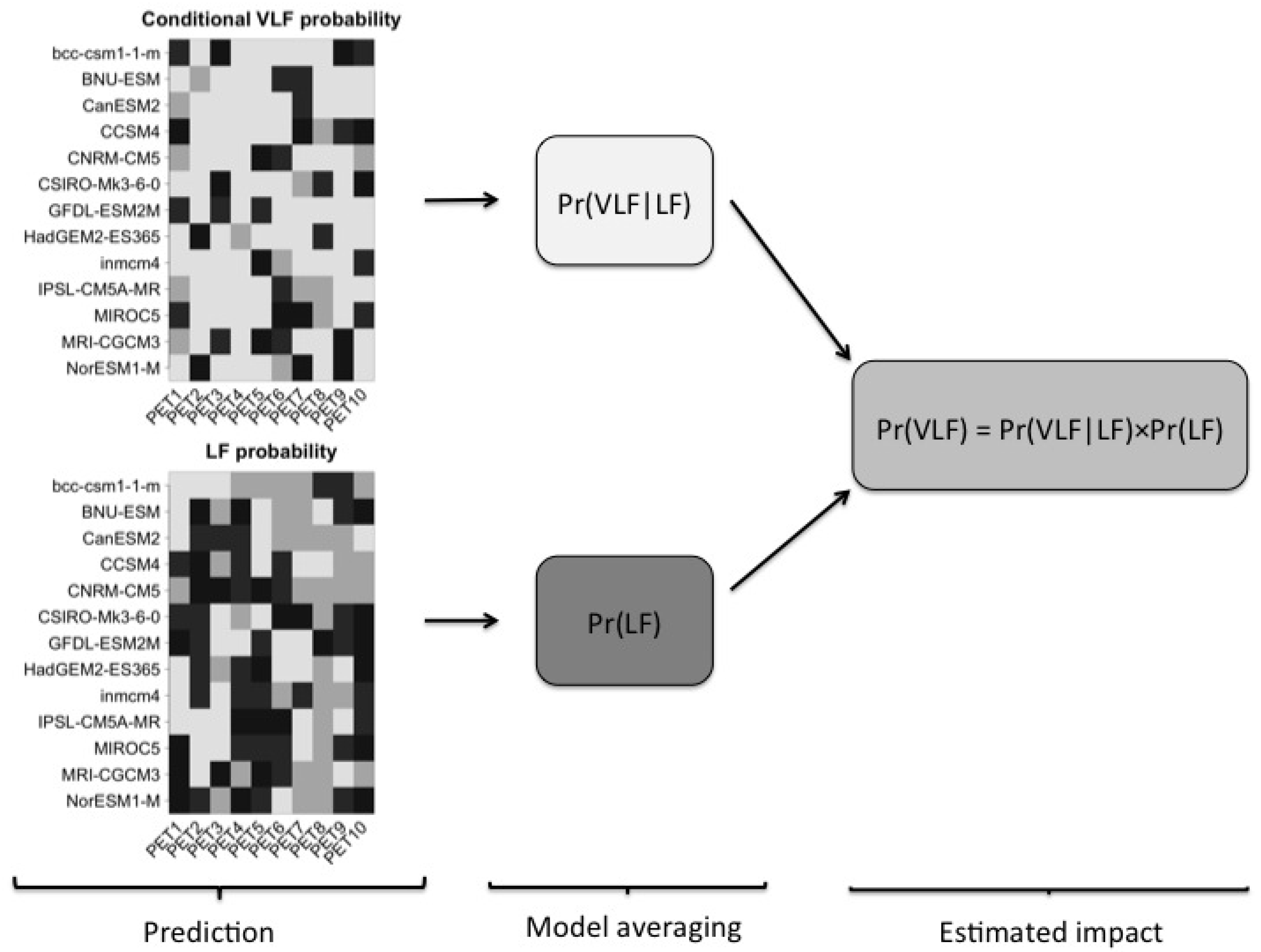
2.4. Multi-Model Very-Large Fire Predictions

The structural uncertainties arising from training PETs to observed meteorological data are compounded by structural uncertainties arising from the application of these models to long-term climate forecasts. To improve the quality of the probability estimates and VLF occurrence forecasts, multi-model averages of fire event probabilities are used to integrate both sources of structural uncertainty: the choice of the PET and selection of the climate model. The final probability estimates are assumed to be an average of predictions from all combination pairs of the 100 PETs within each forest and 13 modeled weather datasets; a total of 1300 individual predictions for each region, month, and probability of interest. The modeled weather data used to make PET predictions come from the second version of regional Multivariate Adaptive Constructed Analogs (MACA) [47] dataset that was trained on gridMET, and downscaled with 13 GCMs: bcc-csm1-1-m, BNU-ESM, CanESM2, CCSM4, CNRM-CM5, CSIRO-Mk3-6-0, GFDL-ESM2M, HadGEM2-ES365, inmcm4, IPSL-CM5A-MR, MIROC5, MRI-CGCM3, NorESM1-M.
The multi-model averages are calculated using both unweighted and weighted approaches. The unweighted approach assigns equal weight to each individual prediction and assumes that each PET and climate model is equally credible. The weighted approach assigns unequal weights to predictions from each pairing of PETs and climate models, to try to bias-correct the multi-model averages and optimize predictive performance. The final weight applied to each individual prediction is the product of two independent components: a climate model weight and a PET weight. For a specified region and month, we can write the estimated probabilities as,
p ¯ L F = i = 1 100 j = 1 13 u L F , i v j p L F , i , j ,
p ¯ V L F = i = 1 100 j = 1 13 u V L F , i v j p V L F , i , j .
Here, u * , i represents the weight applied to the predictions from PET i, v j represents the weight applied to predictions utilizing climate model j, and p * , i , j is the prediction obtained from PET i utilizing climate model j. We estimate the weight components using a fully Bayesian approach that incorporates fire occurrence and modeled climate forcings from 1984–2005, as well as probabilistic representations of possible parameter estimates. Via Bayes rule, we know that the posterior of the model weight components, θ = u L F , u V L F , v , is proportional to the product of the likelihood and prior probability distributions. The likelihood component represents the probability of observing the fire occurrence time series, X = X L F , X V L F , assuming that they were generated from a Bernoulli process parameterized with our weighted multi-model averages:
X L F , t Bernoulli ( p ¯ L F , t ) ,
X V L F , t Bernoulli ( p ¯ V L F , t X L F , t ) .
The prior component, p ( θ ) , which is a probability density function representing our a priori belief regarding the parameter values, is defined using independent Dirichlet priors with uninformative concentration parameters:
u L F , u V L F , v Dirichlet ( 1 ) .
The posterior was approximated using Just Another Gibbs Sampler (JAGS) software (Plummer 2003 [41]) and the runjags package in R (R Development Core Team 2008 [53]). An initial set of 30,000 samples were generated from three parallel Markov Chain Monte Carlo chains using a burn-in interval of 10,000 steps, adaptive phase of 10,000 steps, and thinning interval of 100. Calculations were performed on a MacBook Pro (Quanta Computer, Inc, Shanghai, China) with a 2.7 GHz Intel Core i7 processor (Hillsboro, Oregon, USA). Convergence was monitored visually, and also via the calculation of the potential scale reduction factor, using the range of the central 90th percentile of the marginal posteriors as a test statistic (Brooks and Gelman 1998 [54]). We assume that the second half of the chain has approximately converged if the maximum potential scale reduction factor fell below 1.01. If the chain had not converged, then it was continued in batches of 1000 iterations until the maximum potential scale reduction factor was less than 1.01 (Gelman and Shirley 2011 [55]). To provide guidance to future analysts looking to perform similar analyses, an informal computational comparison of JAGS (Version 4.3.0) and Stan software (Version 2.17.3) was completed, which is described in the supplementary materials. The final VLF probabilities can then be calculated by averaging both probabilities of interest—either with point estimate averages of the model weights or using the full posterior in the weighted approach—and applying Bayes rule (Figure 2). The resulting distribution of VLF probability time series is then used to estimate the changes in VLF frequency in the future by finding the difference between the expected number of VLFs in the historical climate (1956–2005), and the expected number of VLFs in the future (2050–2099) under moderate and severe warming scenarios, RCP 4.5 and RCP 8.5, respectively.

2.5. Ensemble Assessment

The ability of the multi-model averages to estimate observed VLF frequencies was quantified over the temporal range of the extant MTBS fire occurrence record at three non-overlapping time periods. Two of the three time periods correspond to the tuning (1984–2005), training (2006–2015) datasets that were used to bias correct and fit the initial suite of PETs respectively. Additionally, a testing dataset independent of the information used to build the multi-model averages was constructed using 2016 MTBS occurrence data. For each time period, a sample of 100,000 probability time series were drawn from the relevant multi-model average posterior, which were then used to simulate the distribution of VLF counts predicted during that time period. Note that the 2016 fire data used to independently validate the multi-model averages represent an updated version of the MTBS data that was unavailable during the PET training and tuning stages, and that slight differences in the total number of large (>404 hectares) incidents between 1984–2015 were observed in the two versions. Specifically, the original MTBS dataset reported 10,295 large incidents between 1984–2015, while the updated version reported 10,298 large incidents during that same period.

3. Results

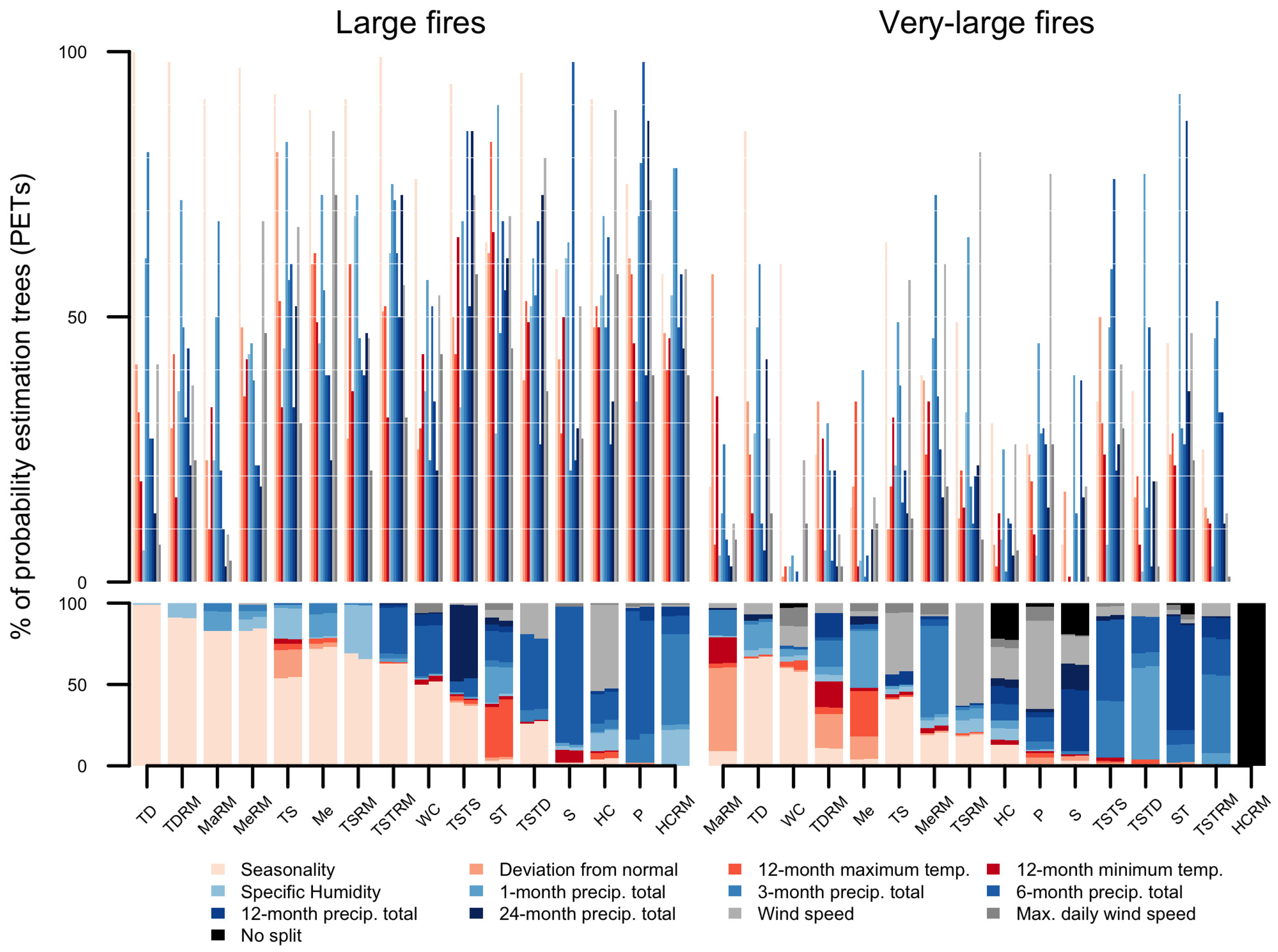
3.1. Important Predictors of Very-Large Fires

The diversity of predictors used in the PETs was high, and the important meteorological variables varied by region, the summary statistic, and the type of fire probability. Temperature metrics, in particular seasonality, are a commonly utilized weather predictor in LF forests, and in 10 of the 16 LF forests, seasonality is present in 90 or more of the PETs. On the other hand, while temperature metrics are frequently utilized when constructing PETs, they are not always the optimal splitting criterion. For instance, in the Savanna, Prairie, and Hot Continental Regime Mountains, precipitation metrics overwhelmingly replace temperature based metrics as the optimal discriminant of large and no fire months, and in other regions such as the Subtropical and Hot Continental Division, this designation is highly uncertain.
The importance of temperature metrics also varied by the type of fire probability considered, with temperature metrics more commonly identified as the optimal split criterion in LF forests compared to VLF forests. This sensitivity of PET structure to the type of fire probability could also arise in other ways. For example, in the Hot Continental Regime Mountains, the LF forest overwhelmingly relies on precipitation metrics for prediction, while the corresponding VLF forest utilizes no predictors and reports a constant conditional VLF probability. Similarly, in the Tropical/Subtropical Regime Mountains and Prairie divisions, conditional VLF forests tended to identify wind metrics as the optimal split criterion much more frequently than in the LF forests. Additionally, PET complexity tended to be lower in VLF forests than in the LF forests. The average number of variables used per PET, size, and the number of leaves were inflated in the latter, and weather invariant null models were only ever observed in the VLF forests. The variability in the optimal splitting criterion was also higher in the VLF forests, suggesting a relative lack of certainty regarding the optimal discriminant in conditional VLF probabilities compared to LF probabilities. Weighting did not appear to drastically influence the relative contribution of the weather predictors within each forest (Figure 3).

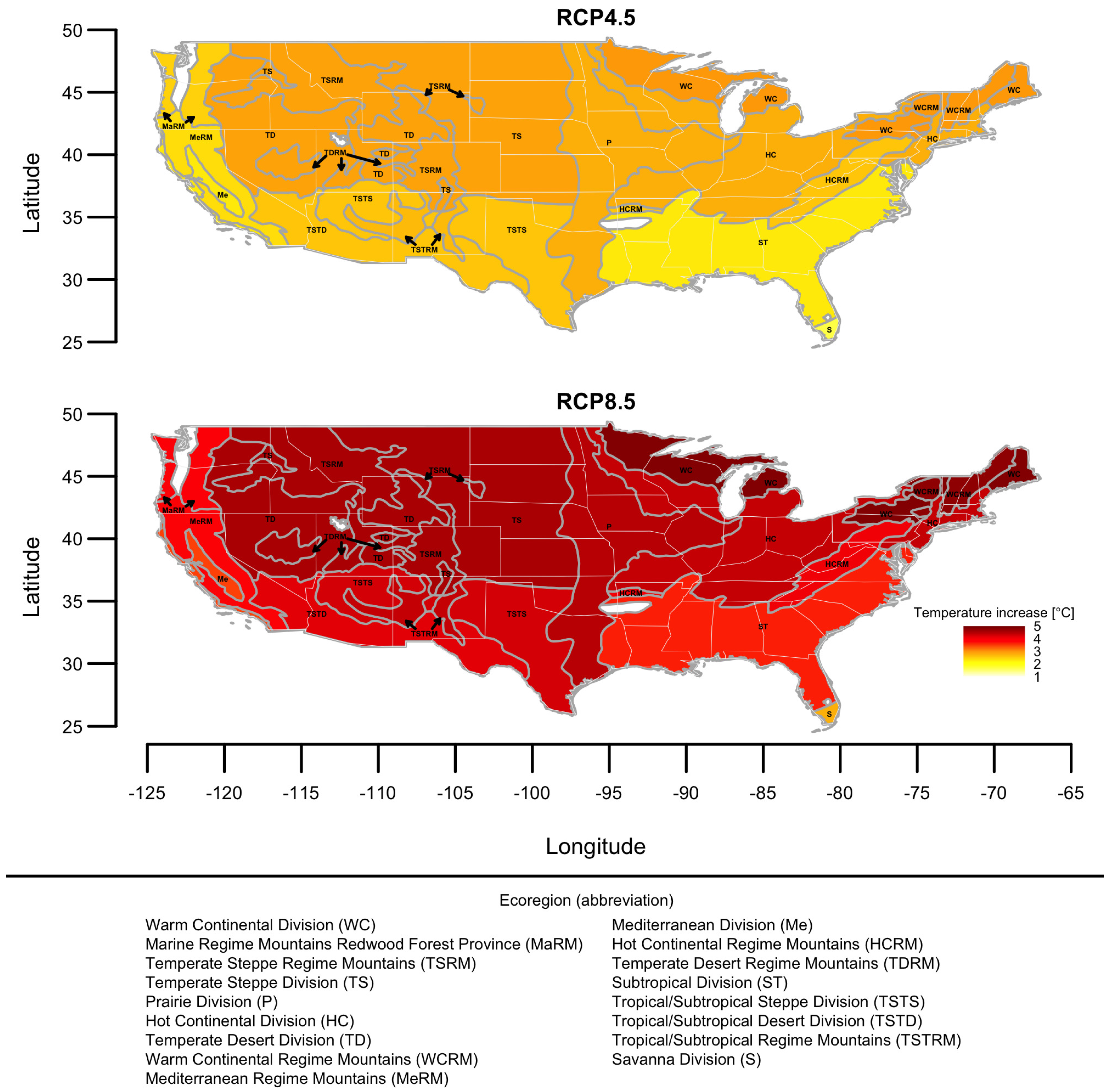
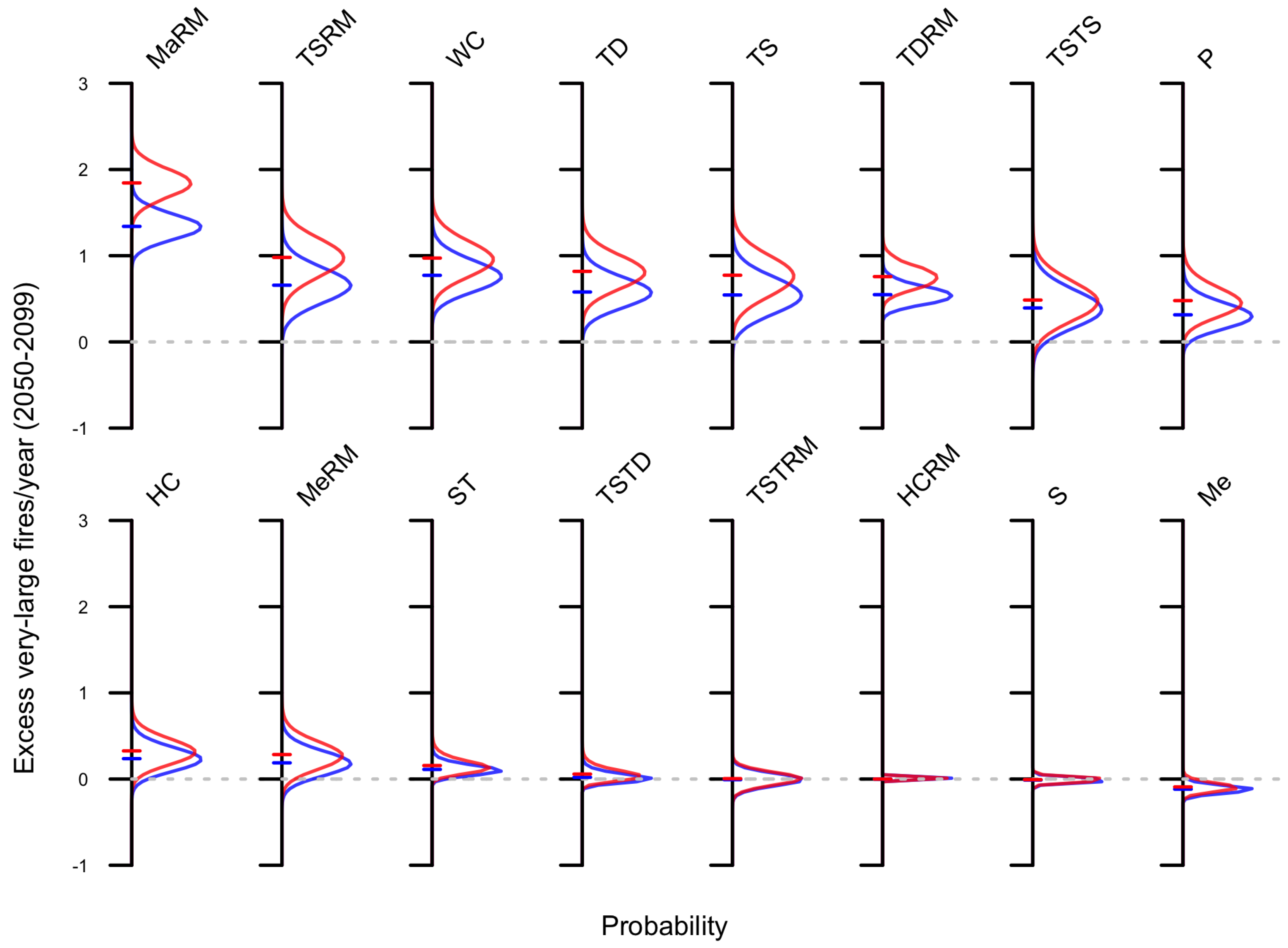
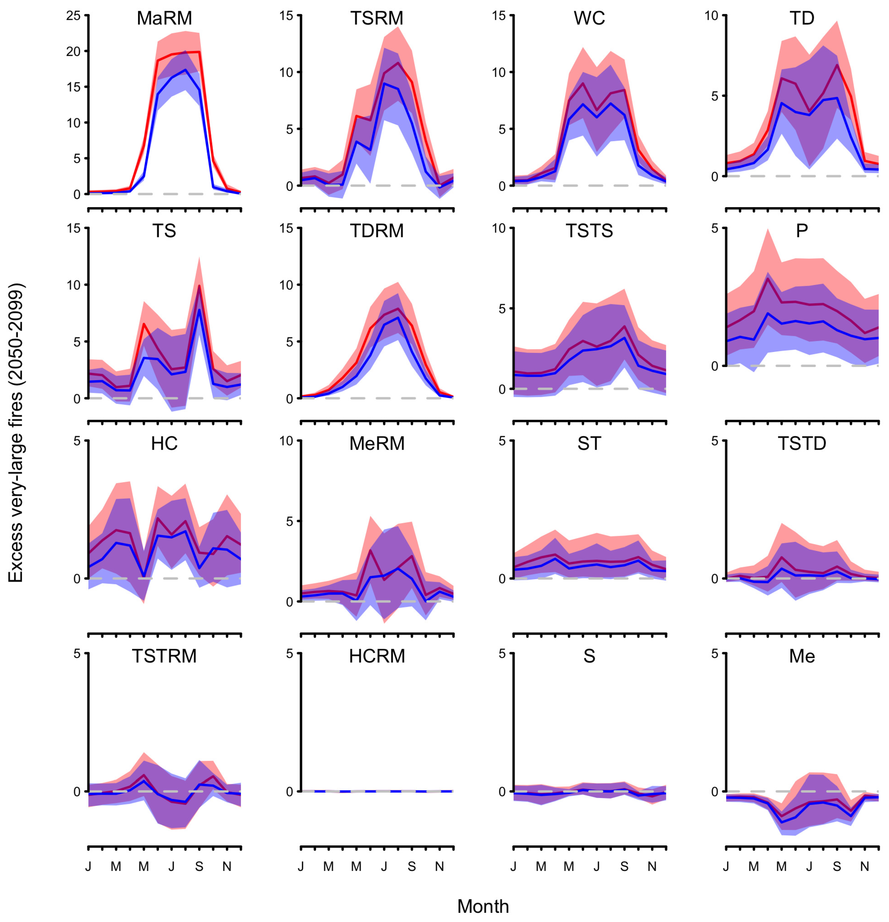
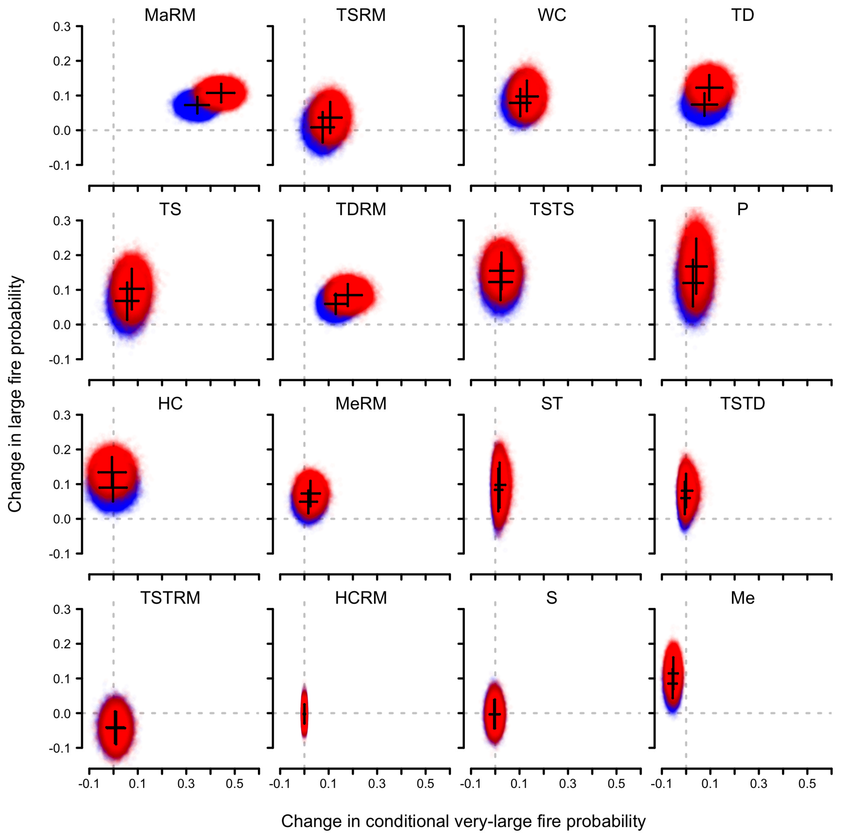
3.2. Climate Change and Very-Large Fire Occurrence

In most divisions, the expected number of VLFs is predicted to increase in 2050–2099 compared to 1956–2005. The Marine Regime Mountains Redwood Forest division is predicted to have the largest absolute increase with about 13 additional fires per decade under the RCP 4.5 scenario and about 18 additional fires per decade under the RCP 8.5 scenario. For most of the regions under consideration, the average predicted increase ranges from near-zero to several additional VLF per decade relative to historical predictions. In some regions, like Mediterranean and Savanna divisions, the multi-model average predicts slight decreases in VLF activity. The largest absolute decrease occurred in Mediterranean California, which is predicted to have about one less VLF per decade relative to historical predictions under both RCP scenarios. In general, increases in VLF frequency are more severe under the RCP 8.5 scenario than under the RCP 4.5 scenario, although the sensitivity to RCP scenario varies by division (Figure 4). The largest absolute difference in average VLFs per decade between the RCP 8.5 and RCP 4.5 scenarios was in the Marine Regime Redwood Forest division, which had about 5 additional VLFs in the RCP 8.5 scenario. Although the Hot Continental Regime Mountains predicts a larger VLF count per decade under the RCP 4.5 scenario than the RCP 8.5, the difference is negligibly small. The median difference between the RCP 8.5 and RCP 4.5 scenario across the 16 ecoregions was 0.9 additional VLFs per decade under the RCP 8.5 scenario.
Future changes in VLF frequency may or may not be uniformly distributed throughout the year. The largest absolute monthly changes in VLF frequency are observed in the Marine Regime Mountain Redwood Forest division during the summer months, while the shoulder months are not predicted to drastically differ from present day VLF frequency. In contrast to the predictions in the Marine Regime Mountain Redwood Forest division, semi-uniform changes in VLF frequency are also predicted in some regions. For instance, the Subtropical division is predicted to have about 6-8 additional VLF events during the last half of the 21st century relative to the 1956–2005 reference period, but shows no strong preference as to what month these events will occur. For nearly all regions and months, VLF frequency is predicted to increase or show no change compared to historical reference conditions, with the Prairie division being an example of the former and the Hot Continental Regime Mountains the latter. The Mediterranean division is an exception to this pattern, as reductions in future very-large fire frequency are predicted from October to May (Figure 5).
The changes in overall VLF frequency are predicted to be a result of changes in both model components: the LF and conditional VLF occurrence probabilities. For divisions like Marine Regime Mountains Redwood Forest, both probabilities increase, implying that the LF months will become increasingly frequent and a larger proportion of the months classified as LF will become VLF months. Other divisions showed increases in only one of the model components. In the Temperate Steppe Regime Mountain division, only conditional VLF probabilities are predicted to increase, and in the Tropical/Subtropical Steppe division, only LF probabilities are anticipated to increase. Significant decreases in the model components are only predicted in the Mediterranean and Tropical Subtropical Regime Mountains divisions, which respectively have decreases in the conditional VLF and LF probability components in 2050–2099 compared to 1956–2005 climate model forcings. The Mediterranean LF probability components are predicted to increase, while the conditional VLF probability component is expected to remain the same in the Tropical Subtropical Regime Mountains division. In general, the changes in model components are greater in the RCP 8.5 scenario compared to the RCP 4.5 scenario, although the differences between the two future scenarios were nearly imperceptible in some regions (Figure 6).

3.3. Ensemble Assessment

The proportion of simulated VLF counts equal to or below the observed values varied by region and time period, and the frequency with which this quantity fell within the central 95th percentile of the simulated VLF counts informs us of the overall quality of the multi-model average forecasts. Using this performance metric, the highest ensemble quality occurs in regions where the central 95th percentile of simulated VLF counts covers the observed VLF counts in all three time periods, which was observed in the Marine Regime Mountains Redwood Forest, Prairie, Hot Continental, Temperate Desert Regime Mountains, and Savanna divisions. In as many regions, this quantity fell in the central 95th percentile for the testing and tuning time periods only, or in the testing and training time periods only. This was observed in the Temperate Steppe Regime Mountains, Temperate Steppe, Temperate Desert, Mediterranean Regime Mountains, and Tropical/Subtropical Steppe divisions. Predictive performance was occasionally poor in the tuning and training time periods, but good during the testing time period, as was observed in the Warm Continental, Subtropical, and Tropical/Subtropical Desert divisions. In the Mediterranean division, the ensembles performed well on the tuning and training time periods, but showed poor performance when predicting data they were not already optimized on. The lowest model quality was seen in the Tropical/Subtropical Regime Mountains, where observed VLF counts were covered by the central 95th percentile in the tuning time period only, and in the Hot Continental Regime Mountains, where the central 95th percentile of the simulated VLF counts never covered the observed quantity.
Consistent underestimation, where the observed VLF count was equal to or greater than the median simulated VLF count in all three time periods, was reported in nine of the sixteen regions considered. The magnitude of these underestimates ranged from very minor, as in the Temperate Desert, to quite severe, as in the Hot Continental Regime Mountains. Consistent overestimates were much less frequently observed, with only the Marine Regime Mountains Redwood Forest and Warm Continental divisions reporting observed VLF counts equal to or less than the median simulated VLF counts in every time period. Five regions had VLF counts that were located to the left or right of the median depending on the time period considered. The Temperate Steppe, Prairie, and Tropical/Subtropical Steppe divisions simulations tended to underestimate the true VLF counts, while the opposite was observed in Temperate Steppe Regime Mountains and Hot Continental divisions.
The simulated distributions did not appear to be strongly sensitive to the choice of RCP scenario during the temporal extent of the training (2006–2015) and testing (2016) time periods, as there are only slight differences between them during those times (Figure 7).

4. Discussion

4.1. Important Predictors of Very-Large Fires

Wildfire events are associated with a number of factors (Flannigan et al., 2009 [28]) that may vary in space (Stavros et al., 2014 [56], Barbero et al., 2015 [57], Arpaci et al., 2013 [58], Flannigan et al., 2006 [59]), and may reveal themselves only under certain conditions (Slocum et al., 2010 [60], Krueger et al., 2015 [61]); it should not then be unexpected that model variability can often be high. Attempts to identify any single factor as most closely associated with VLFs are frustrated by the complex behavior of wildfires, competition among models, data limitations, and diversity of performance criterion. Despite the ubiquity of structural and other uncertainties, the relative importance of various coarse scale meteorological factors to specific wildfire activities could be gauged by observing the frequency with which they were utilized to make predictions. In some cases, a meteorological variable could, with high confidence, be readily identified as important to predicting VLFs in a particular region. In the Temperate Desert division, seasonality was frequently utilized in PETs for both wildfire probabilities, and was also often identified as the optimal splitting criterion. More typically, however, some level of structural uncertainty was present and identifying a best predictor was not always as obvious. In the Subtropical division, LF forest, temperature and precipitation based variables were identified as the optimal splitting criterion with nearly equal frequency. In the Mediterranean Regime Mountains division, seasonality was frequently the optimal splitting criterion in the LF forest, but it was much less common in the VLF forest. Moreover, in the Mediterranean division, wind-based metrics were frequently utilized in LF forests in the Mediterranean forest, but not as a first-split in the PETs. Model variability could be particularly high in the LF forests in the Eastern Continental United States. Precipitation based variables were overwhelmingly preferred in extreme southern Florida and in the Appalachians, but wind based variables were preferred in the Hot Continental division; Temperature was slightly preferred in the Warm Continental division, and as already mentioned, the Subtropical region showed no strong preference with regard splitting criterion. Although some regions showed preferences for certain weather variables, model variability was fairly high in the VLF forests.
Although these structural uncertainties are sometimes obstacles to identifying important meteorological relationships with VLFs, they are also critical to understanding the true level of confidence we have in observed correlations and safeguard against overconfident conclusions. While clearly notable levels of model variability could be encountered across multiple factors, robust patterns and trends could still be inferred. For instance, we note that, in most of the West, with the exception of the Great Plains and the Tropical/Subtropical portions of the Southwest, temperature based metrics were often the best predictor of LFs and were commonly used in LF forests. In the remaining Western areas, temperature metrics were less useful and instead precipitation metrics were selected as the optimal splitting criterion. This apparent preference for precipitation based metrics over temperature based ones in these regions may be related to the characteristics of fuel-limited versus climate-limited fire regimes (Meyn et al., 2007 [32]), or due to a relative inability of seasonal temperature fluctuations to match wildfire activity compared to precipitation. The relative popularity of wind-based variables in very-large forests compared to very-large forests is also interesting, as wind has been reported to have variable influence on wildfire activity depending on fire size and geographic location (Slocum et al., 2010 [60]).

4.2. Climate Change and Very-Large Fire Occurrence

For both RCP scenarios and nearly all divisions, complex changes to wildfire activity are predicted that will result in an overall increase in the frequency of VLFs, which is largely consistent with many other projections (Flannigan et al., 2009 [28], Barbero et al., 2015 [21] ). While overall increases in the frequency of these events are predicted using robust methods, the exact nature of these changes remain unclear. It is not certain, for instance, if the range of fire sizes will remain largely static in the future and only frequency of exceptionally large events will increase; or if the size distribution will shift, so that burn areas exceed historic records. These distinctions are important because the relative costs of these two competing possibilities are likely to vary across decision makers. The Mediterranean division was somewhat of an exception to the overall reported increases in VLF activity. Westerling et al. (2011 [26]) project either no change or modest increases in LF activity in much of lowland California, and large increases in mid- and high-elevation locations, which at first seems inconsistent with the predicted decrease in VLF activity, although there are a few explanations. Firstly, by considering a larger number of climate models and predictive models, the range of results in this analysis will be inherently more variable, and marginal results seen in other studies could emerge as significant when these structural uncertainties are incorporated. Secondly, as shown in this study, the environmental drivers of large and conditional VLF probabilities can vary, and differences regarding the definition of LF can result in variability amongst methodologies (Slocum et al., 2010 [60]). Thirdly, differences between the covariates considered and model structure are likely to alter the predictions across analyses. For instance, anthropogenic and vegetation effects on wildfire activity were omitted in this study, but are known to be an important influence of wildfire activity in California (Syphard et al., 2007 [62]) and elsewhere (Syphard et al., 2017 [63]).
The months in which VLF activity was historically highest may not necessarily apply in the second half of the 21st century, and noticeable changes in intra-annual patterns, usually increases, of VLF activity were predicted in most scenarios and regions. Some regions, like Temperature Desert Regime Mountains and Marine Regime Mountains Redwood Forests, are predicted to have increases in VLF frequency only during a limited portion of the year, while others, like the Subtropical division, are predicted to have a relatively uniform increase in VLF frequency throughout the year. Given that simultaneous increases in VLF probabilities are anticipated in multiple independent regions, it is likely that VLF activity will change in ways that will increase resource strain. Indeed, the results of this study suggest that, depending on the emission scenario, between 12–13 regions will have future VLF frequencies that exceed the historical record, and that intra-annual increases in VLF occurrence are often predicted during the same time of year in spatially distinct regions.
In addition to changes to intra-annual patterns of overall VLF frequency, it is important to acknowledge that the overall increases in VLF frequency are the product of two processes: changes in LF and conditional VLF probabilities. Any increase in VLF frequency is then the result of one of three scenarios: an increase in both probabilities, and increase in LF frequency only, or an increase in the frequency that LFs become VLFs. These specific changes in model components may be of particular relevance to firefighting, public health professionals, and other decision-makers who will—due to differences in the impacts of the events—react to no-fire, LF, and VLF months differently and require guidance regarding the characteristics of the novel future wildfire regimes. Reducing the uncertainty as to which emission scenario the future will resemble should also be a priority for decision-makers and researchers, as the predicted changes tend to be more exaggerated under the RCP 8.5 scenario compared to the RCP 4.5, which should influence adaptation and mitigation efforts of future wildfire impacts.

4.3. Caveats and Future Work

While the simultaneous acknowledgement of structural uncertainties in the climate models and PETs represents an interesting approach, there are still a number of uncertainties that were not addressed in this climate impact analysis. The limited availability of reliable and consistently recorded (e.g., satellite-based) measurements of wildfire activity (Taylor et al., 2013 [64]) and the inherent rarity of VLF events remain significant obstacles to validating predictions and estimating underlying model structures. The validation results should be considered as the current state of knowledge regarding the ensemble’s predictive ability, and may change when more data becomes available in the future. If inter-annual variability in wildfire activity is high, then the validation results used in this study may be based on particularly predictable or unpredictable fire years, and therefore not be representative of the actual performance. Longer duration datasets would be preferred, and thirty year climatologies are often considered ideal (Arguez and Vose 2011 [65]), but the entire range of available burn area data only extends 33 years and it is unlikely that longer time scale meteorological associations with VLF activity will be accurately captured with the relative brevity of data (Westerling and Swetnam 2003 [66], Marlon et al., 2012 [67]). Moreover, if recent increases in VLF activity are indicative of a sudden a shift into overall wildfire patterns unlike what has been observed in the past, then forecasting future activities based on historical relationships could be inadequate. For instance, the two events occurring in the Hot Continental Regime Mountains in 2016 were quite unusual in historical terms, as only four VLF months were reported from 1984–2005, and only one VLF was reported from 2006–2015.
Data limitations may also be qualitative, and many of the remaining important structural uncertainties are due to unconsidered covariates, like vegetation changes, suppression effort, and population growth, that were not modeled due to data inavailability, practical considerations, and challenges related to predicting these quantities in the future. While the PETs used in this study produced a diverse suite of predictive models and are known to be highly unstable (Wang et al., 2016 [50]), there are many other lingering sources of structural uncertainty that could still be incorporated. For instance, generalized linear models could be used instead, which take a number of mathematical structures depending on the choice of link and response functions (Clyde 2003 [68]). Similarly, various data transformations could be used to generate competing models of the wildfire activities. Alternative models could be constructed that condense the two model components into VLF occurrence probabilities only, so that the event space of each month is purely binary. Instead of biogeographical classification of regions, the Continental United States could be partitioned using administrative or other boundaries to generate VLF predictions relevant to specific stakeholders. Hence, clearly a broad variety of other structural uncertainties still exist that could potentially influence predictions of future VLF frequency in the second half of the century.
It is important to understand that the VLF probabilities do not inform us as to what will actually happen, but rather communicates the degree of uncertainty about future outcomes conditional on carbon emission scenarios. For this reason, some tolerance to deviations between observed and expected VLF frequencies should be considered, as should the fact that the predictions were based on modeled climate data as opposed to direct observations. Still, in many regions, the ensemble performance was relatively adequate and the simulated distribution of fire counts covered the observations. Moreover, when deviations occurred, they tended to underestimate the future VLF counts. Hence, the overall claim that VLF counts will increase in the future under climate change is supported by the results of this study, as well as through the work of others (Stavros et al., 2014 [56], Barbero et al., 2015 [21]). Stochastic uncertainty will be critical when explicitly linking changes to VLF occurrence to human activities and for assessing the future levels of VLF simultaneity (Tedim et al., 2018 [69]) and is a factor that would be well addressed using the methods described here, but is beyond the scope of this paper. The inherent stochasticity of the PET construction process suggests that repeated applications of this methodology in the future may yield slight variations to the results presented here.
Interestingly, a standard factor analysis revealed that more than 86 percent of the variability in predicted probabilities could be attributed to variance amongst the PETs rather than variance amongst the climate models, and while the PETs are an inherently unstable choice of predictive model, this suggests that structural uncertainties should receive the attention of climate impact researchers in much the same way that the choice of climate model does. Further exploration of these structural uncertainties in climate impact analyses cannot be recommended enough in future analyses, as they inform not only of future impacts, but the reliability of these predictions, which can influence decision-maker behaviors in a variety of ways (Weber and Johnson 2009 [70]).

5. Conclusions

While the key conclusion from this research was that fires that were historically considered very-large and rare are likely to become increasingly frequent in most regions of the Continental United States at the end of the 21st century, there are also a number of other complexities in future wildfire activity that may be of further relevance to researchers and decision-makers. For instance, although temperature based metrics were often important for prediction, this analysis also found that the identification of important predictors could be highly uncertain across a number of factors, which should be ignored at one’s peril. Moreover, even using the relatively simple probabilistic models we developed, rich details regarding future wildfire activities were constructed that reasonably matched observed fire frequencies and were dynamic in terms of intra-annual trends, fire frequency, simultaneous fire occurrence, and the readiness with which LFs become VLFs. Although overall increases are predicted, we also observed exceptions and regional variability. In the Northwestern United States, VLF frequencies were predicted to increase, with nearly two additional events per year, and increases close to one additional VLF per year were fairly commonly throughout much of the Continental United States as well. In rare instances, the potential for decreases in VLF activity was also reported, most surprisingly in Mediterranean California.
The cumulative impact of these changes are anticipated to affect decision-makers in various ways and the techniques described here have a number of benefits for addressing their needs. For instance, the presented Bayesian model averaging techniques avoids many of the risks of traditional model selection techniques that are especially dangerous when predicting complex phenomena such as wildfire. Moreover, this method simultaneously provides a natural method of calculating important event probabilities that are critical to informed decision-making. While uncertainty in climate models is well understood amongst climate impact researchers, these results highlight the hidden sources of structural uncertainty, and encourage the use of Bayesian model averaging to reconcile them into robust forecasts of future wildfire and other impacts resulting from climate change.

Supplementary Materials

Supplementary File 1

Author Contributions

Conceptualization, N.K.L.; Data curation, N.K.L.; Formal analysis, H.R.P., N.K.L. and E.A.S.; Funding acquisition, N.K.L.; Methodology, H.R.P., N.K.L., E.A.S., A.C. and E.A.; Project administration, N.K.L.; Resources, N.K.L.; Software, H.R.P.; Supervision, N.K.L. and E.A.S.; Visualization, H.R.P., N.K.L. and E.A.S.; Writing—original draft, H.R.P.; Writing—review & editing, H.R.P., N.K.L., E.A.S., A.C. and E.A.. H.R.P. contributed to the paper’s methodology, software, formal analysis, writing—original draft preparation, writing—review and editing, and visualization. N.K.L. contributed heavily to the paper’s conceptualization, methodology, formal analysis, resources, data curation, writing—review and editing, visualization, supervision, project administration, and funding acquisition. E.A.S. contributed to the methodology, formal analysis, writing—review and editing, visualization, and supervision. A.C. and E.A. contributed to the methodology, as well as the writing—review and editing.

Funding

This research was funded by Joint Fire Science Program project number 11-1-7-4 and by the Joint Venture Agreement 13-JV-11261987-094 between the USFS PNW Research Station and the University of Washington.

Acknowledgments

The authors would like to acknowledge John Abatzoglou and Renaud Barbero for their work that was done in parallel with this analysis. We would also like to thank the members of the AirFire team for their continued support and suggestions throughout this project’s lifetime. We are also grateful to the contributions of three anonymous reviewers whose suggestions greatly enhanced the quality of this manuscript.

Conflicts of Interest

The authors declare no conflict of interest.

References

  1. Barrett, K. The Full Community Costs of Wildfire. Headwaters Economics. Available online: https:// headwaterseconomics.org/wp-content/uploads/full-wildfire-costs-report.pdf (accessed on 14 December 2018).
  2. González-Cabán, A. Economic Cost of Initial Attack and Large-Fire Suppression; USDA Forest Service General Technical Report PSW-068; U.S. Department of Agriculture, Forest Service, Pacific Southwest Forest and Range Experiment Station: Berkeley, CA, USA, 1983; 7p.
  3. Stephens, S.L.; Burrows, N.; Buyantuyev, A.; Gray, R.W.; Keane, R.E.; Kubian, R.; Liu, S.; Seijo, F.; Shu, L.; Tolhurst, K.G.; et al. Temperate and boreal forest mega-fires: Characteristics and challenges. Front. Ecol. Environ. 2014, 12, 115–122. [Google Scholar] [CrossRef]
  4. Dale, L. The True Cost of Wildfire in The Western US; Western Forestry Leadership Coalition: Denver, CO, USA, 2009. [Google Scholar]
  5. Neary, D.G.; Gottfried, G.J.; Ffolliott, P.F. Post-wildfire watershed flood responses. In Proceedings of the 2nd International Fire Ecology Conference, American Meteorological Society, Orlando, FL, USA, 28 November–2 December 2003; Volume 65982. [Google Scholar]
  6. Peppin, D.L.; Fulé, P.Z.; Sieg, C.H.; Beyers, J.L.; Hunter, M.E.; Robichaud, P.R. Recent trends in post-wildfire seeding in western US forests: Costs and seed mixes. Int. J. Wildl. Fire 2011, 20, 702–708. [Google Scholar] [CrossRef]
  7. Beverly, J.L.; Bothwell, P. Wildfire evacuations in Canada 1980–2007. Nat. Hazards 2011, 59, 571–596. [Google Scholar] [CrossRef]
  8. Beverly, J.L.; Flannigan, M.D.; Stocks, B.J.; Bothwell, P. The association between Northern Hemisphere climate patterns and interannual variability in Canadian wildfire activity. Can. J. For. Res. 2011, 41, 2193–2201. [Google Scholar] [CrossRef]
  9. Forster, C.; Wandinger, U.; Wotawa, G.; James, P.; Mattis, I.; Althausen, D.; Simmonds, P.; O’Doherty, S.; Jennings, S.G.; Kleefeld, C.; et al. Transport of boreal forest fire emissions from Canada to Europe. J. Geophys. Res. Atmos. 2001, 106, 22887–22906. [Google Scholar] [CrossRef] [Green Version]
  10. Val Martin, M.; Heald, C.L.; Ford, B.; Prenni, A.J.; Wiedinmyer, C. A decadal satellite analysis of the origins and impacts of smoke in Colorado. Atmos. Chem. Phys. 2013, 13, 7429–7439. [Google Scholar] [CrossRef] [Green Version]
  11. Reid, C.E.; Brauer, M.; Johnston, F.H.; Jerrett, M.; Balmes, J.R.; Elliott, C.T. Critical review of health impacts of wildfire smoke exposure. Environ. Health Perspect. 2016, 124, 1334. [Google Scholar] [CrossRef] [PubMed]
  12. Achtemeier, G.L. On the formation and persistence of superfog in woodland smoke. Meteorol. Appl. 2009, 16, 215–225. [Google Scholar] [CrossRef] [Green Version]
  13. Moeltner, K.; Kim, M.K.; Zhu, E.; Yang, W. Wildfire smoke and health impacts: A closer look at fire attributes and their marginal effects. J. Environ. Econ. Manag. 2013, 66, 476–496. [Google Scholar] [CrossRef]
  14. Crawford, J.A.; Wahren, C.H.; Kyle, S.; Moir, W.H. Responses of exotic plant species to fires in Pinus ponderosa forests in northern Arizona. J. Veg. Sci. 2001, 12, 261–268. [Google Scholar] [CrossRef]
  15. Rocca, M.E.; Miniat, C.F.; Mitchell, R.J. Introduction to the regional assessments: Climate change, wildfire, and forest ecosystem services in the USA. For. Ecol. Manag. 2014, 327, 8. [Google Scholar] [CrossRef]
  16. Haffey, C.; Sisk, T.D.; Allen, C.D.; Thode, A.E.; Margolis, E.Q. Limits to Ponderosa Pine Regeneration following Large High-Severity Forest Fires in the United States Southwest. Fire Ecol. 2018, 14, 143–163. [Google Scholar]
  17. Williams, J. Exploring the onset of high-impact mega-fires through a forest land management prism. For. Ecol. Manag. 2013, 294, 4–10. [Google Scholar] [CrossRef]
  18. Dennison, P.E.; Brewer, S.C.; Arnold, J.D.; Moritz, M.A. Large wildfire trends in the western United States. Geophys. Res. Lett. 2014, 41, 2928–2933. [Google Scholar] [CrossRef]
  19. Barbero, R.; Abatzoglou, J.T.; Steel, E.A.; Larkin, N.K. Modeling very large-fire occurrences over the continental United States from weather and climate forcing. Environ. Res. Lett. 2014, 9, 124009. [Google Scholar] [CrossRef] [Green Version]
  20. Stavros, E.N.; Abatzoglou, J.T.; McKenzie, D.; Larkin, N.K. Regional projections of the likelihood of very large wildland fires under a changing climate in the contiguous Western United States. Clim. Chang. 2014, 126, 455–468. [Google Scholar] [CrossRef]
  21. Barbero, R.; Abatzoglou, J.T.; Larkin, N.K.; Kolden, C.A.; Stocks, B. Climate change presents increased potential for very large fires in the contiguous United States. Int. J. Wildl. Fire 2015, 24, 892–899. [Google Scholar] [CrossRef]
  22. Chen, J.; Brissette, F.P.; Poulin, A.; Leconte, R. Overall uncertainty study of the hydrological impacts of climate change for a Canadian watershed. Water Resour. Res. 2011, 47. [Google Scholar] [CrossRef] [Green Version]
  23. Morgan, M.G.; Henrion, M.; Small, M. Uncertainty: A Guide to Dealing With Uncertainty in Quantitative Risk and Policy Analysis; Cambridge University Press: Cambridge, UK, 1992. [Google Scholar]
  24. Syphard, A.D.; Sheehan, T.; Rustigian-Romsos, H.; Ferschweiler, K. Mapping future fire probability under climate change: Does vegetation matter? PLoS ONE 2018, 13, e0201680. [Google Scholar] [CrossRef] [PubMed]
  25. Sitch, S.; Huntingford, C.; Gedney, N.; Levy, P.E.; Lomas, M.; Piao, S.L.; Betts, R.; Cias, P.; Cox, P.; Friedlingstein, P.; et al. Evaluation of the terrestrial carbon cycle, future plant geography and climate-carbon cycle feedbacks using five Dynamic Global Vegetation Models (DGVMs). Glob. Chang. Biol. 2008, 14, 2015–2039. [Google Scholar] [CrossRef]
  26. Westerling, A.L.; Bryant, B.P.; Preisler, H.K.; Holmes, T.P.; Hidalgo, H.G.; Das, T.; Shrestha, S.R. Climate change and growth scenarios for California wildfire. Clim. Chang. 2011, 109, 445–463. [Google Scholar] [CrossRef]
  27. Taylor, K.E.; Stouffer, R.J.; Meehl, G.A. An overview of CMIP5 and the experiment design. Bull. Am. Meteorol. Soc. 2012, 93, 485–498. [Google Scholar] [CrossRef]
  28. Flannigan, M.D.; Krawchuk, M.A.; de Groot, W.J.; Wotton, B.M.; Gowman, L.M. Implications of changing climate for global wildland fire. Int. J. Wildl. Fire 2009, 18, 483–507. [Google Scholar] [CrossRef]
  29. Allen, C.D.; Macalady, A.K.; Chenchouni, H.; Bachelet, D.; McDowell, N.; Vennetier, M.; Kitzberger, T.; Rigling, A.; Breshears, D.D.; Hogg, E.H.; et al. A global overview of drought and heat-induced tree mortality reveals emerging climate change risks for forests. For. Ecol. Manag. 2010, 259, 660–684. [Google Scholar] [CrossRef]
  30. Bentz, B.J.; Régnière, J.; Fettig, C.J.; Hansen, E.M.; Hayes, J.L.; Hicke, J.A.; Kelsey, R.G.; Negrón, J.F.; Seybold, S.J. Climate change and bark beetles of the western United States and Canada: Direct and indirect effects. BioScience 2010, 60, 602–613. [Google Scholar] [CrossRef]
  31. Westerling, A.L. Increasing western US forest wildfire activity: Sensitivity to changes in the timing of spring. Philos. Trans. R. Soc. B 2016, 371, 20150178. [Google Scholar] [CrossRef] [PubMed]
  32. Meyn, A.; White, P.S.; Buhk, C.; Jentsch, A. Environmental drivers of large, infrequent wildfires: The emerging conceptual model. Prog. Phys. Geogr. 2007, 31, 287–312. [Google Scholar] [CrossRef]
  33. De Groot, W.J.; Johnston, J.; Jurko, N.; Cantin, A.S. Fuel moisture sensitivity to temperature and precipitation: Climate change implications. Clim. Chang. 2016, 134, 59–71. [Google Scholar]
  34. Bradley, B.A.; Curtis, C.A.; Chambers, J.C. Bromus response to climate and projected changes with climate change. In Exotic Brome-Grasses in Arid and Semiarid Ecosystems of the Western US; Springer International Publishing: New York, NY, USA, 2016; pp. 257–274. [Google Scholar]
  35. Zargar, A.; Sadiq, R.; Naser, B.; Khan, F.I. A review of drought indices. Environ. Rev. 2011, 19, 333–349. [Google Scholar] [CrossRef]
  36. Holsinger, L.; Parks, S.A.; Miller, C. Weather, fuels, and topography impede wildland fire spread in western US landscapes. For. Ecol. Manag. 2016, 380, 59–69. [Google Scholar] [CrossRef]
  37. Mallick, B.K.; Gelfand, A.E. Generalized linear models with unknown link functions. Biometrika 1994, 81, 237–245. [Google Scholar] [CrossRef] [Green Version]
  38. Littell, J.S.; McKenzie, D.; Kerns, B.K.; Cushman, S.; Shaw, C.G. Managing uncertainty in climate-driven ecological models to inform adaptation to climate change. Ecosphere 2011, 2, 1–19. [Google Scholar] [CrossRef]
  39. Raftery, A.E.; Zheng, Y. Discussion: Performance of Bayesian model averaging. J. Am. Stat. Assoc. 2003, 98, 931–938. [Google Scholar] [CrossRef]
  40. Fragoso, T.M.; Bertoli, W.; Louzada, F. Bayesian model averaging: A systematic review and conceptual classification. Int. Stat. Rev. 2018, 86, 1–28. [Google Scholar] [CrossRef]
  41. Plummer, M. JAGS: A program for analysis of Bayesian graphical models using Gibbs sampling. In Proceedings of the 3rd International Workshop on Distributed Statistical Computing, Vienna, Austria, 20–22 March 2003. [Google Scholar]
  42. Carpenter, B.; Gelman, A.; Hoffman, M.D.; Lee, D.; Goodrich, B.; Brubaker, M.; Guo, J.; Betancourt, M.; Li, P.; Riddell, A. Stan: A probabilistic programming language. J. Stat. Softw. 2017, 76. [Google Scholar] [CrossRef]
  43. Rue, H.; Martino, S.; Chopin, N. Approximate Bayesian inference for latent Gaussian models by using integrated nested Laplace approximations. J. R. Stat. Soc. 2009, 71, 319–392. [Google Scholar] [CrossRef] [Green Version]
  44. Monnahan, C.C.; Thorson, J.T.; Branch, T.A. Faster estimation of Bayesian models in ecology using Hamiltonian Monte Carlo. Methods Ecol. Evol. 2017, 8, 339–348. [Google Scholar] [CrossRef]
  45. Monitoring Trends in Burn Severity. Available online: http://www.mtbs.gov (accessed on 21 November 2017).
  46. Bailey, R.G. Bailey’s ecoregions and subregions of the United States, Puerto Rico, and the U.S. Virgin Islands; Forest Service Research Data Archive: Fort Collins, CO, USA, 2016. Available online: https://doi.org/10.2737/RDS-2016-0003 (accessed on 14 December 2018).
  47. Climatology Lab. Available online: http://www.climatologylab.org (accessed on 29 January 2018).
  48. Weiss, A.; Hays, C.J. Calculating daily mean air temperatures by different methods: Implications from a non-linear algorithm. Agric. For. Meteorol. 2005, 128, 57–65. [Google Scholar] [CrossRef]
  49. Provost, F.; Domingos, P. Well-Trained PETs: Improving Probability Estimation Trees, CeDER Working Paper #IS-00-04, Stern School of Business; New York University: New York, NY, USA, 2000. [Google Scholar]
  50. Wang, H.; Yang, F.; Leu, Z. An experimental study of the intrinsic stability of random forest variable importance measures. BMC Bioinf. 2016, 17, 60. [Google Scholar] [CrossRef] [PubMed]
  51. Quinlan, J.R. C4.5: Programs for Machine Learning; Elsevier: Amsterdam, The Netherlands, 2014. [Google Scholar]
  52. Hido, S.; Kashima, H.; Takahashi, Y. Roughly balanced bagging for imbalanced data. Statistical Analysis and Data Mining: ASA Data Sci. J. 2009, 2, 412–426. [Google Scholar] [CrossRef] [Green Version]
  53. Development Core Team R. A Language and Environment for Statistical Computing. 2008. Available online: http://www.R-project.org (accessed on 14 December 2018).
  54. Brooks, S.P.; Gelman, A. General methods for monitoring convergence of iterative simulations. J. Comput. Gr. Stat. 1998, 7, 434–455. [Google Scholar]
  55. Gelman, A.; Shirley, K. Inference from simulations and monitoring convergence. In Handbook of Markov chain Monte Carlo; CRC Press: Boca Raton, FL, USA, 2011; pp. 163–174. [Google Scholar]
  56. Stavros, E.N.; Abatzoglou, J.; Larkin, N.K.; McKenzie, D.; Steel, E.A. Climate and very large wildland fires in the contiguous western USA. Int. J. Wildl. Fire 2014, 23, 899–914. [Google Scholar] [CrossRef] [Green Version]
  57. Barbero, R.; Abatzoglou, J.T.; Kolden, C.A.; Hegewisch, K.C.; Larkin, N.K.; Podschwit, H. Multi-scalar influence of weather and climate on very large-fires in the Eastern United States. Int. J. Climatol. 2015, 35, 2180–2186. [Google Scholar] [CrossRef]
  58. Arpaci, A.; Eastaugh, C.S.; Vacik, H. Selecting the best performing fire weather indices for Austrian ecoregions. Theor. Appl. Climatol. 2013, 114, 393–406. [Google Scholar] [CrossRef] [PubMed] [Green Version]
  59. Flannigan Mike, D. Forest fires and climate change in the 21 st century. Mitig. Adapt. Strateg. Global Chang. 2006, 11, 847–859. [Google Scholar] [CrossRef]
  60. Slocum, M.G.; Beckage, B.; Platt, W.J.; Orzell, S.L.; Taylor, W. Effect of climate on wildfire size: A cross-scale analysis. Ecosystems 2010, 13, 828–840. [Google Scholar] [CrossRef]
  61. Krueger, E.S.; Ochsner, T.E.; Engle, D.M.; Carlson, J.D.; Twidwell, D.L. Soil Moisture Affects Growing-Season Wildfire Size in the Southern Great Plains. Soil Sci. Soc. Am. J. 2015, 79, 1567–1576. [Google Scholar] [CrossRef]
  62. Syphard, A.D.; Radeloff, V.C.; Keeley, J.E.; Hawbaker, T.J.; Clayton, M.K.; Stewart, S.I.; Hammer, R.B. Human influence on California fire regimes. Ecol. Appl. 2007, 17, 1388–1402. [Google Scholar] [CrossRef] [PubMed]
  63. Syphard, A.D.; Keeley, J.E.; Pfaff, A.H.; Ferschweiler, K. Human presence diminishes the importance of climate in driving fire activity across the United States. Proc. Natl. Acad. Sci. USA 2017, 201713885. [Google Scholar] [CrossRef] [PubMed]
  64. Taylor, S.W.; Woolford, D.G.; Dean, C.B.; Martell, D.L. Wildfire prediction to inform fire management: Statistical science challenges. Stat. Sci. 2013, 28, 586–615. [Google Scholar] [CrossRef]
  65. Arguez, A.; Vose, R.S. The definition of the standard WMO climate normal: The key to deriving alternative climate normals. Bull. Am. Meteorol. Soc. 2011, 92, 699–704. [Google Scholar] [CrossRef]
  66. Westerling, A.L.; Swetnam, T.W. Interannual to decadal drought and wildfire in the western United States. EOS 2003, 84, 545–555. [Google Scholar] [CrossRef]
  67. Marlon, J.R.; Bartlein, P.J.; Gavin, D.G.; Long, C.J.; Anderson, R.S.; Briles, C.E.; Brown, K.J.; Colombaroli, D.; Hallett, D.J.; Power, M.J.; et al. Long-term perspective on wildfires in the western USA. Proc. Natl. Acad. Sci. USA 2012, 109, E535–E543. [Google Scholar] [CrossRef] [PubMed]
  68. Clyde, M. Model averaging. Subject. Object. Bayesian Stat. 2003, 25, 320–326. [Google Scholar]
  69. Tedim, F.; Leone, V.; Amraoui, M.; Bouillon, C.; Coughlan, M.R.; Delogu, G.M.; Fernandes, P.M.; Ferreira, C.; McCaffrey, S.; McGee, T.K.; et al. Defining extreme wildfire events: Difficulties, challenges, and impacts. Fire 2018, 1, 9. [Google Scholar] [CrossRef]
  70. Weber, E.U.; Johnson, E.J. Decisions under uncertainty: Psychological, economic, and neuroeconomic explanations of risk preference. Neuroeconomics 2009, 2009, 127–144. [Google Scholar]
Figure 1. Map of multi-model mean temperature changes between 1955–2005 and 2050–2099 over the relevant Bailey’s divisions under the representative concentration pathway (RCP) 4.5 (top) and RCP 8.5 emission scenarios (bottom). Regions with insufficient fire occurrence data for analysis are colored white.
Climate 06 00100 g001
Figure 2. Workflow of very-large fire probability calculations. In the prediction phase, probability estimates are calculated for every combination pair of climate model and probability estimation tree. The model-averaging phase combines these predictions into probability estimates using either a weighted or unweighted averages. The final phase uses Bayes rule to calculate the very-large fire probability as the product of both components from the model-averaging phase.
Climate 06 00100 g002
Figure 3. Summary statistics of each forest of probability estimation trees. The top panels show the percentage of probability estimation trees (PETs) in each forest that uses a particular weather predictor for at least one split. The bottom panels show the percentage of PETs for which a weather predictor is selected as the optimal splitting criterion. The relative contribution of each first-split variable under the unweighted (left) and weighted (right) averaging methods are displayed side-by-side.
Climate 06 00100 g003
Figure 4. Kernel density estimates of the posterior and mean of the number of additional very-large fires per year relative to the 1956–2005 reference period per year by ecoregion under the representative concentration pathway (RCP) 4.5 (blue) and RCP 8.5 (red) scenarios arranged by magnitude of change. The excess very-large fire frequency is calculated by randomly sampling ( n = 10 6 ) from the posterior of historical (1956–2005) and future (2050–2099) multi-model averages and calculating the difference.
Climate 06 00100 g004
Figure 5. Predicted intra-annual changes in very-large fire frequency across sixteen biogeographical regions within the Continental United States under the RCP 4.5 (blue) and RCP 8.5 (red). The central 90th percentile and mean of the excess very-large fires are based on 1,000,000 random samples of the posterior multi-model average very-large fire probabilities from the historical (1956–2005) and future (2050–2099) scenarios.
Climate 06 00100 g005
Figure 6. Simulated change in monthly multi-model large-fire and conditional very-large fire probability estimates across biogeographical divisions of the continental United States. The point cloud is a sample of 100,000 differences in average posterior probability components under the historical (1956–2005) and future scenarios (2050–2099); with the RCP 8.5 scenario colored red and RCP 4.5 colored blue. The solid black lines represent the central 90th percentile and the dashed lines are horizontal and vertical lines passing through the origin.
Climate 06 00100 g006
Figure 7. Simulated and actual very-large fire month counts for each region and three time periods: 1984–2005, 2006–2015, and 2016. A sample of 100,000 simulated very-large fire (VLF) counts are produced under historical (grey), RCP 4.5 (blue), and RCP 8.5 (red) scenarios by randomly selecting a VLF probability time series from the posterior and randomly generating a VLF occurrence time series. The observed VLF counts are represented with arrows.
Climate 06 00100 g007
Table 1. Very-large fire cutoffs, the number of fires, large fire months, and very-large fire months for two time periods: 1984–2005 and 2006–2015.
DomainDivision95th Size Percentile (ha)Total # of Fires# of Large Fire Months# of Very-Large Fire Months
’84-’05’06-’15’84-’05’06-’15’84-’05’06-’15
DryTemperate Desert (TD)16,0071623833119552219
Temperate Desert Regime Mountains (TDRM)11,76512178523154
Temperate Steppe (TS)11,664464347119701313
Temperate Steppe Regime Mountains (TSRM)19,853798541101561413
Tropical/Subtropical Desert (TSTD)11,6163652549457109
Tropical/Subtropical Regime Mountains (TSTRM)13,169168143714577
Tropical/Subtropical Steppe (TSTS)10,243388546126791016
TemperateHot Continental (HC)6180267756741112
Hot Continental Regime Mountains (HCRM)458616945302741
Marine Regime Mountains Redwood Forest Province (MaRM)21,776136130483365
Mediterranean (Me)10,98014964823563
Mediterranean Regime Mountains (MeRM)17,772799374143601617
Prairie (P)6707155275475659
Subtropical (ST)5908431312149821614
Subtropical Regime Mountains (SRM)392741631201
Warm Continental (WC)64667320401214
HumidSavanna (S)20,6238945442452

