Article

Projected Changes in Precipitation, Temperature, and Drought across California’s Hydrologic Regions in the 21st Century

California Department of Water Resources, 1416 9th Street, Sacramento, CA 95814, USA
*
Author to whom correspondence should be addressed.
Climate 2018, 6(2), 31; https://doi.org/10.3390/cli6020031
Submission received: 21 March 2018 / Revised: 14 April 2018 / Accepted: 20 April 2018 / Published: 23 April 2018
(This article belongs to the Special Issue Climate Variability and Change in the 21th Century)

Abstract

:
This study investigated potential changes in future precipitation, temperature, and drought across 10 hydrologic regions in California. The latest climate model projections on these variables through 2099 representing the current state of the climate science were applied for this purpose. Changes were explored in terms of differences from a historical baseline as well as the changing trend. The results indicate that warming is expected across all regions in all temperature projections, particularly in late-century. There is no such consensus on precipitation, with projections mostly ranging from −25% to +50% different from the historical baseline. There is no statistically significant increasing or decreasing trend in historical precipitation and in the majority of the projections on precipitation. However, on average, precipitation is expected to increase slightly for most regions. The increases in late-century are expected to be more pronounced than the increases in mid-century. The study also shows that warming in summer and fall is more significant than warming in winter and spring. The study further illustrates that, compared to wet regions, dry regions are projected to become more arid. The inland eastern regions are expecting higher increases in temperature than other regions. Particularly, the coolest region, North Lahontan, tends to have the highest increases in both minimum and maximum temperature and a significant amount of increase in wet season precipitation, indicative of increasing flood risks in this region. Overall, these findings are meaningful from both scientific and practical perspectives. From a scientific perspective, these findings provide useful information that can be utilized to improve the current flood and water supply forecasting models or develop new predictive models. From a practical perspective, these findings can help decision-makers in making different adaptive strategies for different regions to address adverse impacts posed by those potential changes.

1. Introduction

Understanding hydroclimatic changes and trends is of important scientific and practical significance for water resources management [1,2]. In particular, this understanding helps: (1) characterize the behavior of hydroclimatic variables (e.g., precipitation and temperature) as well as extreme events (e.g., droughts); (2) inform the development and enhancement of predictive tools to forecast future occurrence of these events; and (3) develop mitigation and adaptation plans to minimize the adverse impacts of unavoidable changes. This is particularly critical in arid and semi-arid areas including the State of California.
As the home to more than 37 million people [3] and a top-ten economy in the world, California’s growth has been largely dependent on its ability to manage limited water resources [4]. In California, most of the precipitation falls in the northern half of the state, while the majority of the demand comes from the southern half where most of the population and farmlands are located. In addition, available water for supply in the state mostly comes during the wet season (November to April) as most precipitation falls in this period, while the demand is typically the highest in the dry season (late spring and summer) [5]. Furthermore, the state is prone to hydroclimatic extremes [1], with the most recent examples being the record-setting 2012–2015 drought and flooding in 2017. In the face of the geographically and temporally uneven distribution of water resources, the state traditionally relies on statewide and regional water storage and transfer projects, including the State Water Project (SWP) and the Central Valley Project (CVP), to redistribute water to meet multiple and often competing water management objectives [6]. However, the system was designed using hydroclimatic data of the first half of the 20th century. Since then, significant changes have been observed and reported, including increasing temperature, declining mountain snowpack, earlier snowmelt and streamflow peaking, higher percentage of precipitation falling as rainfall rather than snowfall, and increasing sea level, among others [7,8,9,10,11,12,13,14,15,16,17]. Those changes would likely amplify and accelerate in the future as the state’s hydroclimate continues to change in a changing climate. In addition, as the population and economy continue to grow, natural hazards including extreme flooding and drought events pose a greater risk [18,19]. Those factors collectively make reliable water supply and drought and flood management in the state unprecedentedly challenging [20].
In light of their importance, many studies have focused on characterizing potential future hydroclimatic events in California [21,22,23,24,25,26,27,28,29,30]. These studies mostly used climate model projections from the Coupled Model Intercomparison Project Phase 3 (CMIP3) [31], which were produced more than a decade ago and do not represent the latest climate science. There are a few exceptions [21,24,25] that employed the latest climate model projections from the Coupled Model Intercomparison Project Phase 5 (CMIP5) [32]. However, these studies generally focused on spatial scales not directly relevant to water resources management practices. For instance, Sun et al. [24] selected mountainous areas in Southern California as their study focus. In addition, the linear regression approach was generally used in trend assessment in those studies. The results of this method are largely affected by the starting and ending values of the study data and subject to the assumption of normality.
The objective of this study was to provide an assessment of the changes (from historical baseline) and trends of projected precipitation and temperature along with the trends in projected drought over California. This study extended beyond relevant previous studies in terms of: (1) focusing on the scale consistent with the water resources planning and management practices in the state; (2) using climate projections that reflects the latest climate science; and (3) applying the widely-used non-parametric Mann–Kendall approach in trend analysis. Compared to the traditional linear regression method, this method requires less assumption on data distribution and is less affected by the beginning and ending values of the study data. Specifically, the current study was built upon a previous study [14] that explored changes in historical precipitation, temperature, and drought in California. However, the current study differs from [14] in terms of study variables, study metrics, study method, study period, and study purpose. Particularly, this study aimed to offer insight into potential changes to California’s hydroclimate on the scale meaningful for water resources management practices and to inform decision-makers in developing strategies to cope with these changes.

2. Materials and Methods

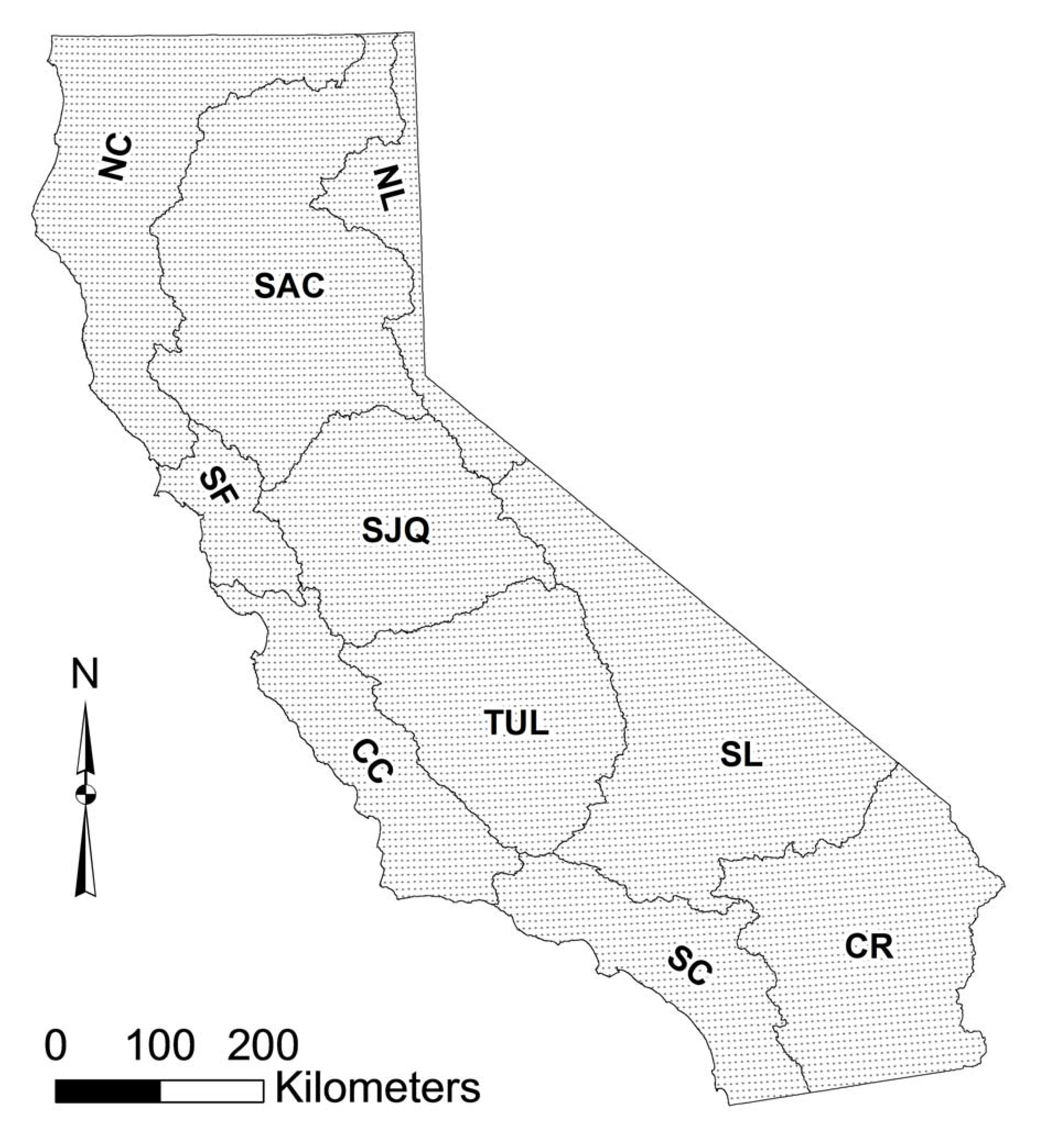
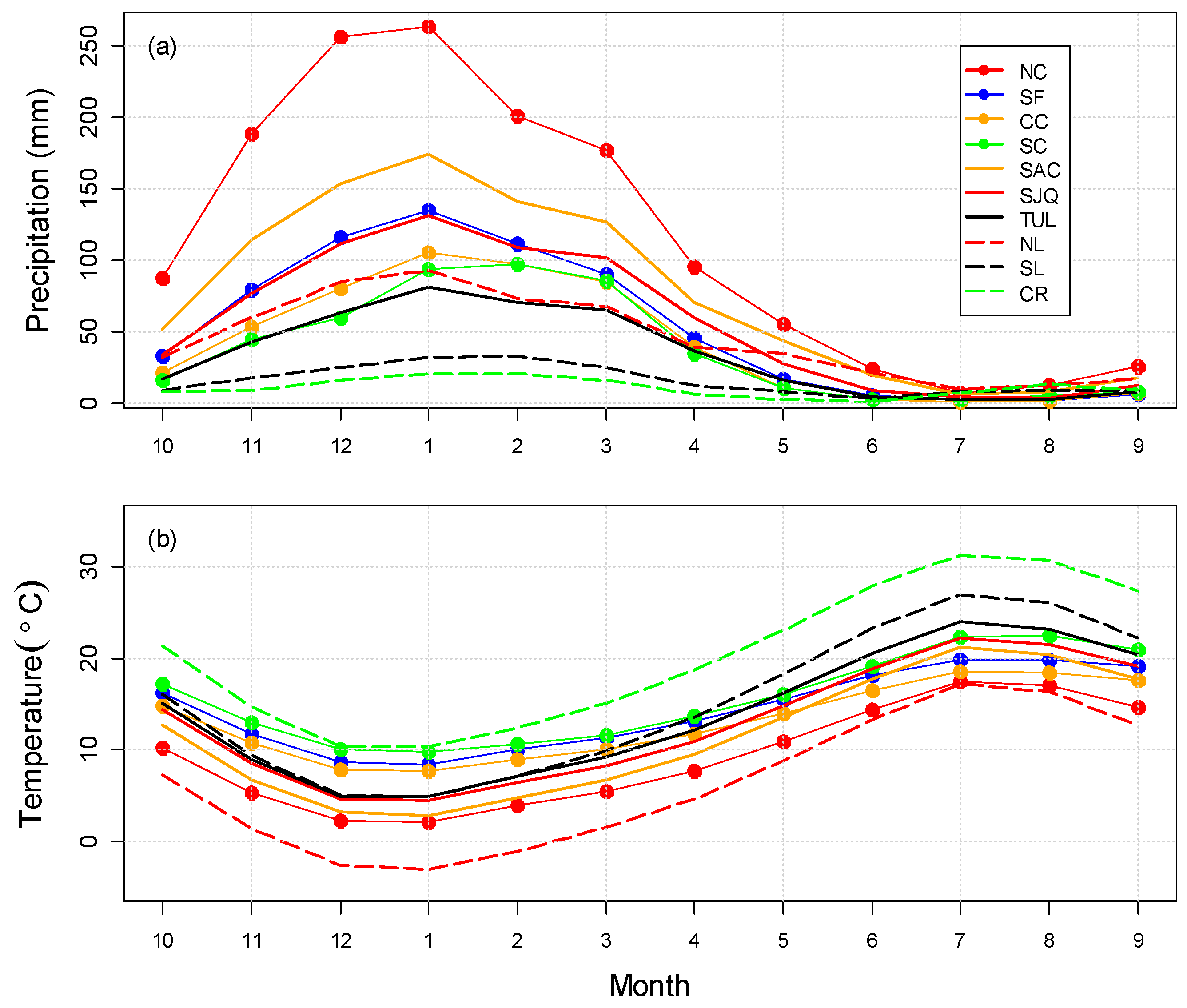
2.1. Study Area and Dataset

Different from the previous study [14] that looks at seven climatic divisions in California, the current study focuses on the 10 hydrologic regions (Figure 1 and Table 1) defined by the California Department of Water Resources (DWR) for operational water resources planning and management purposes [5]. These regions include four coastal regions (North Coast, San Francisco Bay, Central Coast, and South Coast), three Central Valley regions (Sacramento River, San Joaquin River, and Tulare Lake), and three Eastern regions (North Lahontan, South Lahontan, and Colorado River). For each of these three categories (Coastal, Central Valley, and Eastern), climate tends to be drier towards the southern regions.
The North Coast region contains the California Coast Ranges, the Klamath Mountains, and parts of the Modoc Plateau [5]. The eastern side of the region is mostly mountainous with crests around 1800 m (6000 ft) and a few more than 2400 m (8000 ft) in elevation. It is the wettest region in terms of annual precipitation received (1390 mm; Table 1). As such, the region is prone to flooding. Major floods were recorded in 1955, 1964, 1986, 1997, 2006, and 2017. The San Francisco Bay region is the smallest in size. It is bounded by the Pacific Ocean on the west and Coast Ranges on the east where the peaks are above 1200 m (4000 ft) in elevation. The region faces multiple water management challenges including an unreliable water supply, declining water quality and ecosystems, increasing flood risks, and threats posed by sea level rise to coastal areas. The Central Coast region is the most groundwater-dependent region. Groundwater supplies about 80% of its total water usage. The water management challenges of this region include managing groundwater quality and overdraft, sea water intrusion, and flood risks. The South Coast region is the most urbanized and populous region. It accounts for about 7% of the state’s total area but accommodates more than half of the state’s population. As a result, water supply is always a concern of local water managers. The region is also prone to flooding including debris flows and mud slides, particularly in areas where hillsides have been damaged by wildfires. It is the driest and warmest region in the coastal regions (Table 1).
Central Valley regions are the major water supply sources for the state, of which the Sacramento River region is the primary source. It is the largest and second wettest region (925 mm/year; Table 1) of all 10 hydrologic regions. It contributes a majority portion of the water supplied to the SWP and CVP. The region is bounded by Coast Ranges on the west and Sierra Nevada on the east. In this region, about one in three residents is exposed to a 500-year flood event. The region has approximately $65 billion of assets, 1.2 million acres of farmland, and over 340 sensitive species [5]. Major floods in the region normally originate from extreme atmospheric river events during the winter. The San Joaquin River region receives less precipitation than the Sacramento River region. It is also bordered by the Sierra Nevada on the east. However, Sierra Nevada watersheds in this region are higher in elevation, making them more dominated by snow compared to Sacramento River region watersheds. Floods in this region come from both winter rainfall and melting Sierra snowpack [5]. The Tulare Lake region is the driest in the Central Valley and one of the driest regions in the state. It is the largest agricultural region in the state heavily relying on groundwater and imported water supply. Groundwater pumping in this region accounts for more than 38% of the state’s total annual groundwater extraction. The region is also prone to floods caused by winter rainfall and spring snowmelt.
The eastern regions are the least populous. The North Lahontan region accommodates approximately 0.3% of the state’s population. It comprises arid high desert (1200–1500 m in elevation) in the north and the eastern slopes of the Sierra Nevada (up to 3750 m in elevation) in the central and southern portions. It is the coolest region in the state (Table 1). In contrast, the Colorado River region is the hottest. It is also the driest region, receiving only about one tenth of the precipitation received by the North Coast region. The Colorado River region is, however, also subject to flooding which threatens about 38% of its population. Different from all other regions, most flooding events occur from infrequent but high-intensity summer storms in this region. The South Lahontan region is the second driest region in the state. Precipitation for this region comes from both winter storm events and summer thunderstorms.
In general, California has a typical Mediterranean-like climate, with the summer (winter) being dry and warm (cool and wet). This is evident for the 10 regions on the monthly scale (Figure 2). Most of the precipitation occurs during the wet season (November to April). During that period, those regions receive 69% (Colorado River region) to 91% (Central Coast region) of their total annual precipitation. Statewide, 85% of annual precipitation occurs during the wet season. January normally observes the highest amount of precipitation while July is typically the driest month. Meanwhile, January is the coolest month while July has the highest average temperature. South Lahontan and Central Coast regions have the largest (22.1 °C) and smallest (10.1 °C) variations in monthly temperature, respectively. Across all regions, the Colorado River region is the driest and hottest. The North Lahontan region is the coolest and the North Coast region is the wettest. Those observations are consistent with values shown in Table 1.
This study looked at both the historical and projected precipitation, and maximum and minimum temperature data. The projections for 2020–2099 were based on climate model simulations from the Coupled Model Intercomparison Project Phase 5 (CMIP5) [32], which represents the current state of the climate science. Specifically, 20 individual projections from 10 Climate Circulation Models (GCMs) under two newly developed emission scenarios named Representative Concentration Pathways (RCP) 4.5 and RCP 8.5 [33] were selected for the analyses. These 10 GCMs (Table 2) were chosen by DWR Climate Change Technical Advisory Group and deemed as the most suitable for California climate and water resources assessment [34]. RCP 4.5 (RCP 8.5) assumes low (high) future greenhouse-gas concentrations. These projections were downscaled to a very high spatial resolution at 1/16th degree (approximately 6 by 6 km, or 3.75 by 3.75 miles) to better capture the spatial variability of the climate via the Localized Constructed Analogs (LOCA) method [35]. This dataset is made available for California’s Fourth Climate Change Assessment (http://cal-adapt.org/). There are other ways of selecting representative GCMs models [36,37] for water planning analysis. However, they are beyond the scope of this study which exclusively used the GCMs recommended by the CCTAG. These 20 CCTAG-recommended projections have been applied in DWR’s and the California Water Commission’s planning activities including the Central Valley Flood Protection Plan [38] and the Water Storage Investment Program [39]. There is no consensus that some of those projections are more likely to occur than the remaining projections in the future. As a result, these projections are typically treated equally in planning activities. In this study, we looked at these 20 projections together. When looking at the mean of future projections on the annual scale, however, the 10 RCP 4.5 projections and 10 RCP 8.5 projections were analyzed separately.
The gridded historical observational dataset of these three variables on daily scale for water years 1951–2013 of Livneh et al. [40] (https://data.nodc.noaa.gov/) were employed as the historical baseline. The spatial resolution (1/16th degree) of this dataset is consistent with that of the LOCA-downscaled climate model projections. This dataset has been applied extensively in hydrologic modeling and drought assessment [41,42,43,44], and deemed as the best available historical data at this spatial resolution. In this study, both projected and historical datasets were aggregated from grid scale to (hydrologic) regional scale in the analyses presented below.

2.2. Study Method and Metrics

2.2.1. Difference from the Baseline

This study employed difference as a parsimonious metric to represent changes in future conditions from historical conditions. This is a standardized metric applied extensively in climate change related studies [29]. Specifically, the 40-year period, 1951–1990, was used as the historical baseline period. Compared to late 1990s and early 2000s, this period is relatively less impacted by anthropogenic climate change. Additionally, this 40-year window allows enough sample size to represent a wide range of natural variability in hydroclimatic variables. Similar studies have normally used 30-year periods [34]. Two 40-year future periods, mid-century (2020–2059) and late-century (2060–2099), were considered. Mean annual precipitation, and maximum and minimum temperature in the baseline period and future periods were computed and compared. Differences (from the baseline) were subsequently derived. Specifically, when looking at precipitation variables, the focus was on relative differences (i.e., percent different from the baseline); for temperature variables, absolute difference (in degree Celsius) was used.
In addition to annual precipitation and temperature, wet season precipitation and seasonal temperature were also applied as important indices in planning studies [45]. Wet season precipitation accounts for a majority portion of the annual precipitation. Seasonal temperature typically affects water supply and demand. For instance, spring temperature impacts snowmelt timing and amount. Summer temperature impacts evapotranspiration demand. Changes in wet season precipitation and seasonal temperature were also explored in this study.

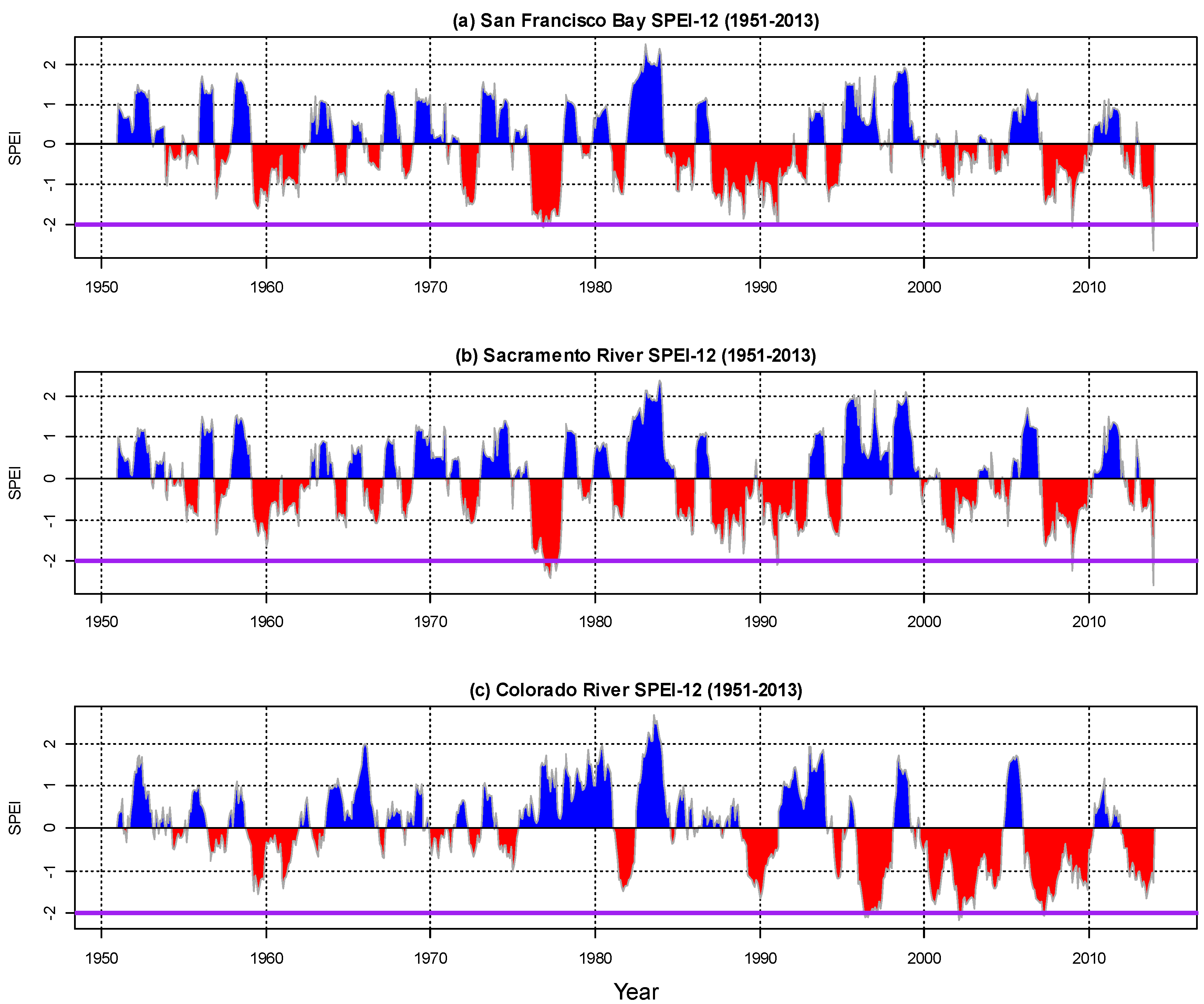
2.2.2. Drought Index

Numerous drought indices have been developed for drought monitoring, assessment and prediction purposes [46,47,48]. Among these indices, the most widely used index might be the Standardized Precipitation Index (SPI) [49] because of its parsimonious (only requiring precipitation as input) and standardized (can be used across different spatial and temporal scales) nature. Despite its popularity, more and more studies noted that evapotranspiration also plays an important role in drought development [50,51,52]. This is particularly true in a warming climate for dry regions where evapotranspiration is an important component of the water budget. For instance, the most recent 2012–2015 California drought was a typical “warm drought” characterized by record-low precipitation and snowpack as well as record-high temperature [45,53,54,55]. As a result, SPI may not be the most appropriate index for drought analysis in California which contains many arid or semi-arid areas.
Most recently, based on the same concept employed in defining the SPI, Vicente-Serrano et al. [56] proposed a Standardized Precipitation-Evapotranspiration Index (SPEI). It first calculates the discrepancies between precipitation (P) and potential evapotranspiration (PET) on a monthly time scale (D = P − PET). Monthly discrepancies can be aggregated to other time scales (e.g., 3-month, 6-month, 12-month, among others) to calculate SPEI values at corresponding temporal scales. Next, a three-parameter Log-logistic distribution is selected to model the discrepancy time series. The probability distribution function of D is calculated according to the fitted Log-logistic distribution (F(x)). Lastly, the SPEI value is determined as the standardized values of F(x) following the approximation of Abramowitz and Stegun [57]:
S P E I = W   C 0 + C 1 W + C 2 W 2 1 + d 1 W + d 2 W 2 + d 3 W 3
where W = 2 ln ( p ) ; p is the probability of exceeding a determined D value; and C0, C1, C2, d1, d2, and d3 are preset constant coefficients. A positive (negative) SPEI value indicates wet (drought) conditions. Depending on the specific values, a drought event can be classified into different categories. Typically, a SPEI value less than −2 indicates extreme drought conditions. A value ranging from −2 to −1 denotes moderate drought conditions. A SPEI greater than −1 but less than 0 represents mild drought conditions.
SPEI has been shown to be a robust index. It compares favorably to other popular drought indices [58,59,60,61,62,63]. The PET is calculated using the Thornthwaite equation [64] which only requires temperature data as input. As such, the SPEI index implicitly considers the impact of temperature on drought situation, making it suitable in assessing drought conditions in future warming scenarios (represented by different model projections in the current study). For detailed explanations on the concept and calculation of the SPEI index, the readers are referred to [56]. The SPEI values on annual scale (SPEI-12), two-year scale (SPEI-24), three-year scale (SPEI-36), and four-year scale (SPEI-48) were chosen in this study. Drought occurs in California at those time scales regularly. It is meaningful to look at future drought at those scales for adaptive planning purpose.
Figure 3 exemplifies the SPEI-12 calculated for the three representative regions from each of the coastal, Central Valley, and eastern areas in the historical period: (1) the highly urbanized San Francisco Bay region; (2) the largest water supply source of the State: Sacramento River region; and (3) the driest Colorado River region. The San Francisco Bay region and the Sacramento River region have similar patterns due to their geographic proximity. The SPEI index for both regions well captures the 1983 and 1997 wet conditions as well as the 1976–1977, 1988–1992, 2007–2009, and the 2012–2013 droughts. The Colorado River region differs from those two regions in terms of annual precipitation (driest) and temperature (hottest). Long-duration droughts occur more frequently after 1990s in this region.

2.2.3. Trend Analysis

The methods applied in climatic and hydrological trend analysis are typically classified into two types: parametric and non-parametric [65,66]. The latter normally requires fewer assumptions (e.g., normality of study data) compared to the former. In reality, the assumptions on data distribution are difficult to satisfy. Therefore, the parametric methods are considered less robust than the non-parametric methods [66]. Among all non-parametric methods, the Mann–Kendall test (MKT) [67,68] has been applied extensively in the field of climatology and hydrology [14,15,16,45,69,70]. The approach first identifies the sign of each possible pair of data in the study time series, followed by the determination of the corresponding test statistic z. The null hypothesis (H0) assumes no significant monotonic trend in the time series while the alternative hypothesis suggests otherwise. The null hypothesis is rejected when |Z| > Z1−α/2, where Z1−α/2 is the probability of the standard normal distribution at a significance level of α. This study employed the MKT in assessing the significance of a trend and uses 0.05 as the significance level.
This study further applied the non-parametric Theil–Sen approach (TSA) [71,72] to identify the slope of significant trends determined via the MKT. In this approach, the slope values (vector T S ) of all data pairs are first calculated:
T S = V i V j i j   i = 1 , 2 , , n ; j = 1 , 2 , , n ; i > j
where n is the length of study record period; and V i and V j are time series values at time i and j , respectively ( i > j ). The median of T S is then used as overall slope of the trend identified for the study time series. A positive (negative) slope value represents an increasing (decreasing) trend. In this study, trend analysis is conducted in both historical (1951–2013) and future periods (2020–2099).

3. Results

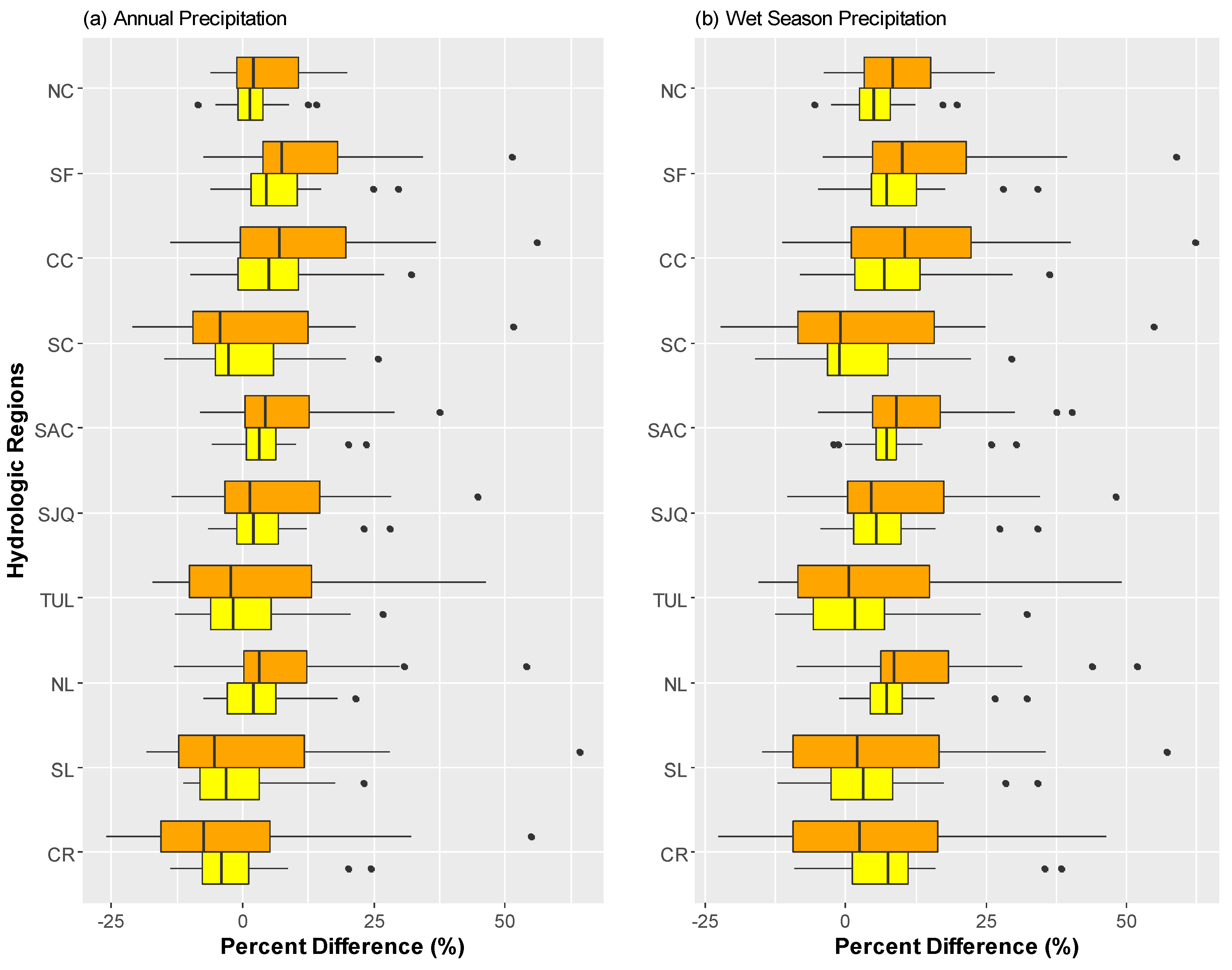
3.1. Differences from the Baseline

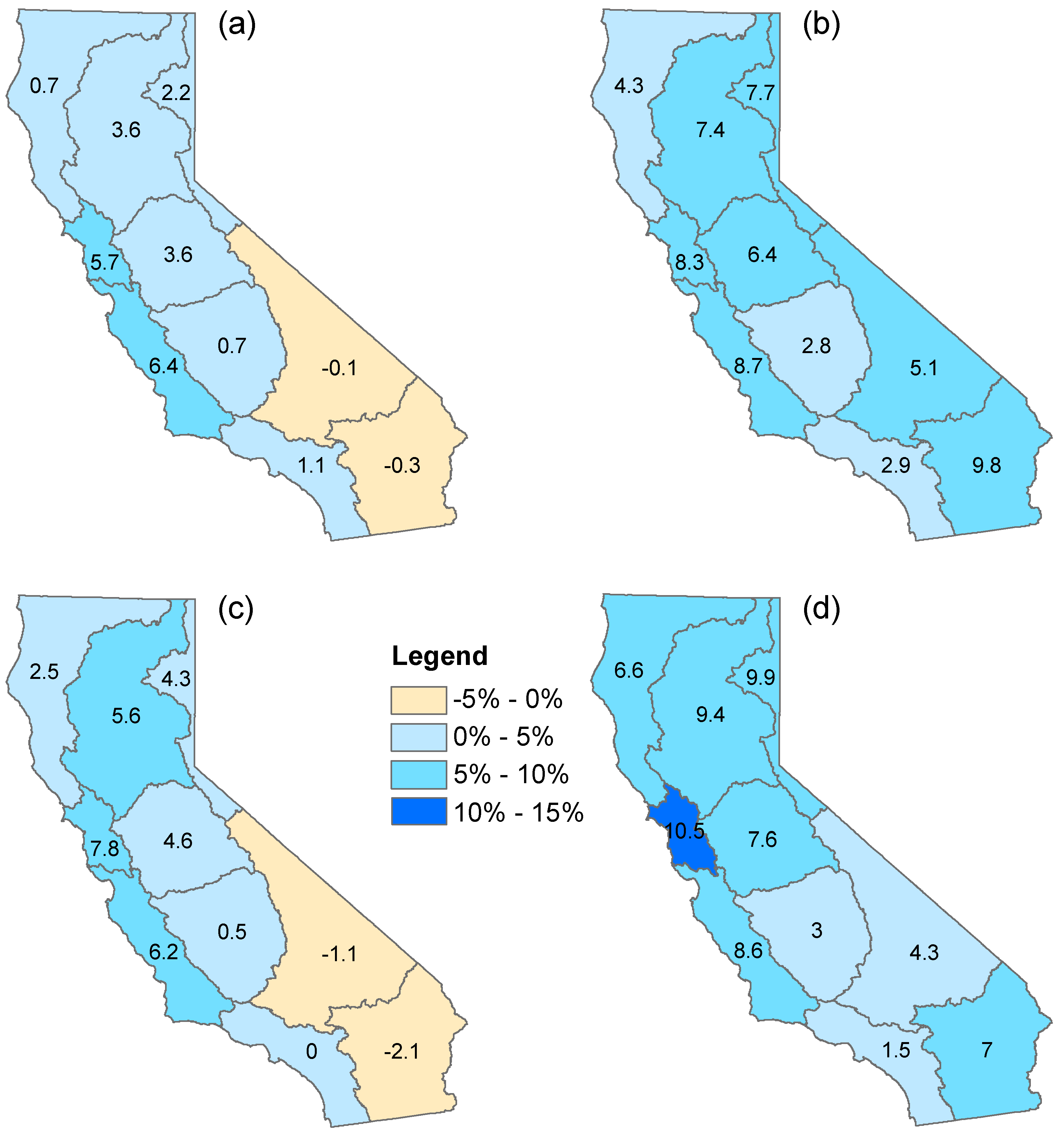
3.1.1. Precipitation
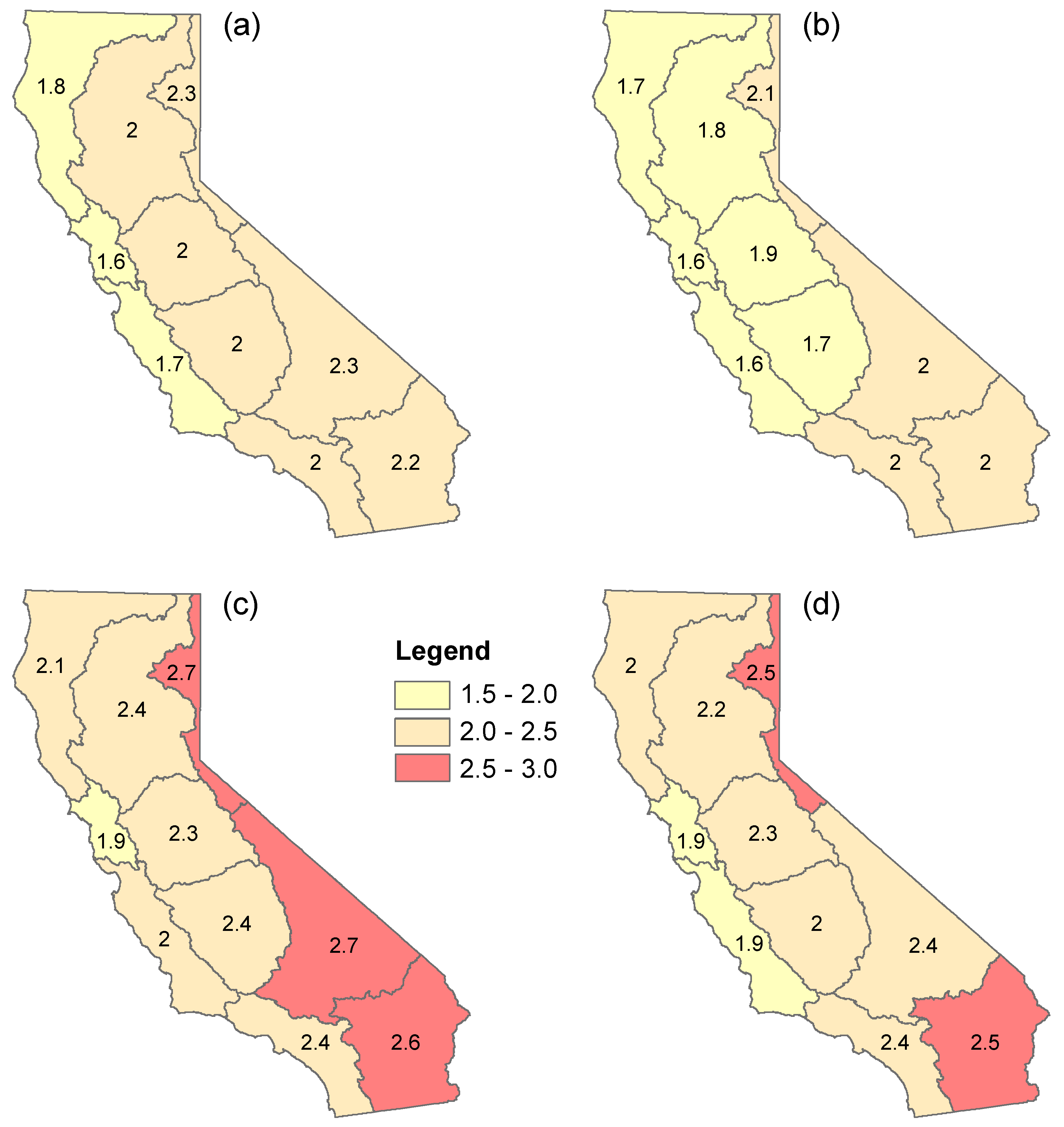
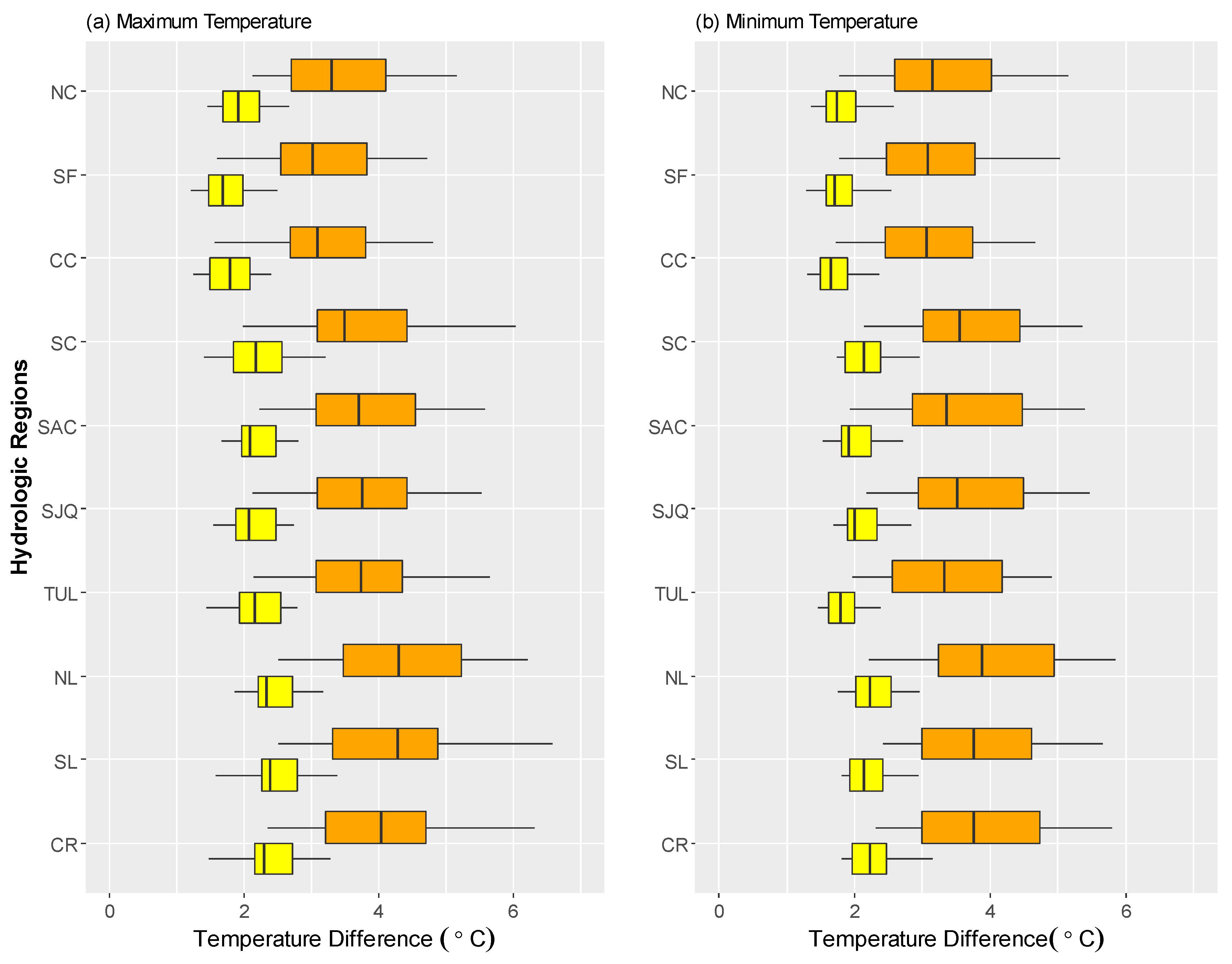
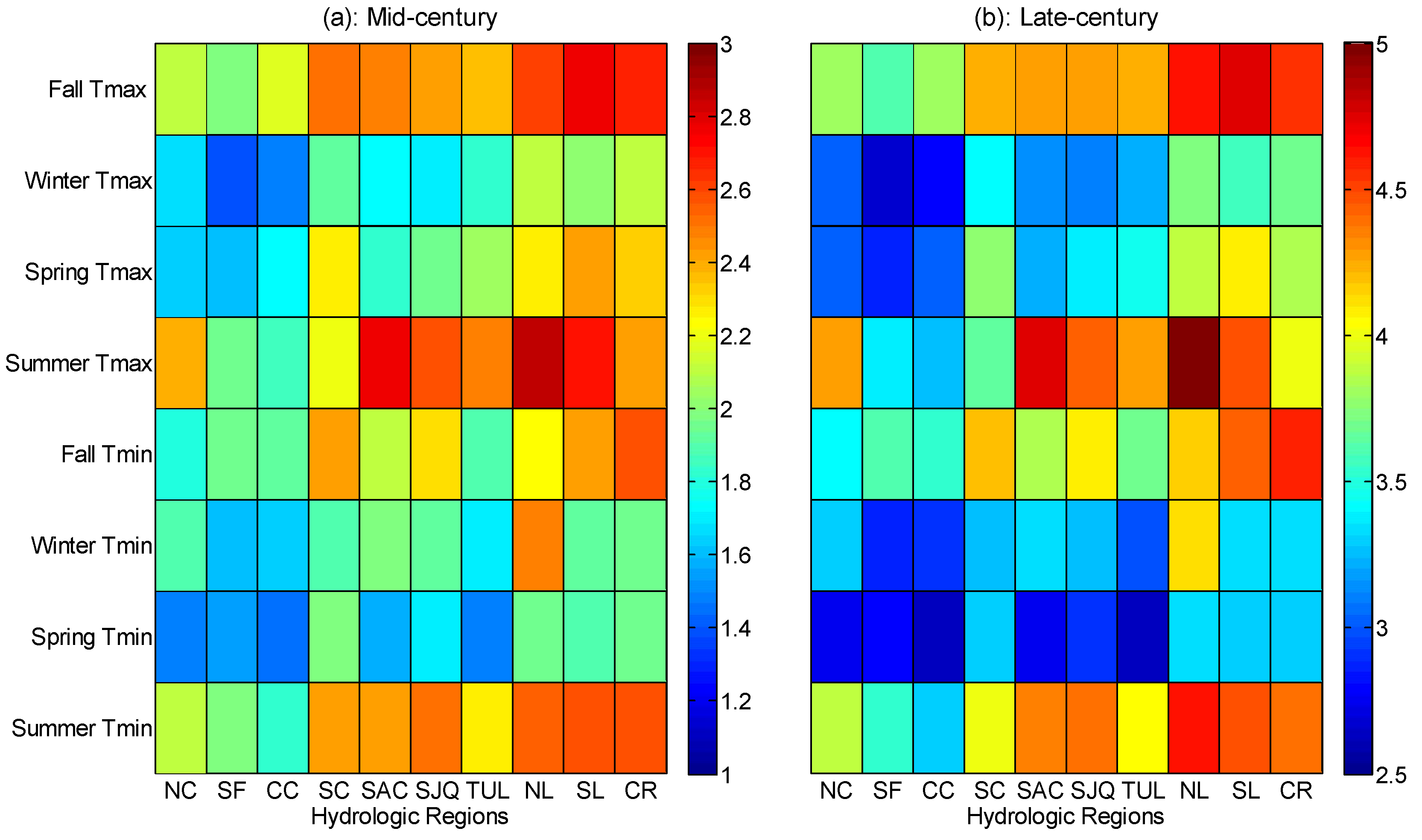
Figure 4 shows the percent differences between historical precipitation and mean (of 10 individual RCP 4.5 projections) projected precipitation in mid-century (Figure 4a,b) and late-century (Figure 4c,d), respectively, on both the annual scale (Figure 4a,c) and during the wet season (Figure 4b,d). It is evident that all regions are expecting increases in precipitation during the wet season, with increases ranging from 2.8% (1.5%) to 9.8% (10.5%) in mid-century (late-century). This observation implies that future storms in the wet season would likely become more frequent, which is in line with the findings of previous studies [25,28]. On the annual scale, most regions are also projected to receive more precipitation, except for the driest two regions: South Lahontan and Colorado River. This suggests that those two regions are expecting much less precipitation in the dry season, although more precipitation is projected for them during the wet season. Typically, summer monsoons are a major contributor to dry season precipitation in these two regions [73,74]. This finding denotes that future monsoons over both regions are likely to become weaker or more sporadic. Across all regions, the San Francisco Bay and the South Coast generally have the highest and lowest increases in precipitation in late-century, respectively, on both temporal scales. This indicates that they are the most and least prone to changes in future storms during this period, respectively, yet they are not the wettest or driest regions. Comparing two future periods, the late-century period is generally expecting a higher increase in precipitation than the mid-century period except for the dry regions including Colorado River, South Lahontan, and South Coast.
The differences between historical precipitation and mean RCP 8.5 precipitation projections are also explored (Table 3). Similar to what Figure 4 indicates, wet season precipitation is expected to increase in both mid-century and late-century across all regions. Increases are expected for annual precipitation for most regions except for three dry regions (i.e., Colorado River, South Lahontan, and South Coast) in mid-century and one region (i.e., Colorado River) in late-century. The increases in late-century are higher. Comparing annual precipitation and wet season precipitation, changes in the latter is more significant in terms of magnitude, which is in line with the RCP 4.5 results as illustrated in Figure 4. Comparing two future periods, changes in the late-century is more pronounced compared to those of the mid-century. Comparing differences of the mean RCP 4.5 projections from the historical baseline and that of the mean RCP 8.5 projections, the latter are more notable. Those are expected since the late-century (compared to mid-century) and the RCP 8.5 scenarios (compared to RCP 4.5 ones) are both expecting higher increases in temperature (Section 3.1.2). A warmer atmosphere can hold more water moisture, indicative of more water available for precipitation.
In addition to looking at the mean of PRC 4.5 and RCP 8.5 projections, individual projections are also investigated (Figure 5) to provide insights on the potential range of precipitation changes. Overall, on both temporal scales, there is no consensus that all projections show increases or decreases consistently for any region in mid-century or in late-century. This finding is also reported in previous studies using old climate projections [22,26,27,28]. The changes mostly range from −25% to 50%, with a few outliers showing more than 50% increases in precipitation. Those outliners come from a single wet climate model under the higher greenhouse-gas emission scenario (RCP 8.5). The variation range is generally larger for late-century (compared to mid-century) and dry regions (compared to wet regions). Additionally, wet season precipitation shows larger change ranges compared to annual precipitation. These results indicate more uncertainties in the projections for the dry regions, in the wet season, and in late-century.

3.1.2. Temperature

Mean annual maximum temperature and minimum temperature are examined in a similar way to the precipitation. The mean of 10 RCP 4.5 projections in two future periods are compared with their counterparts in the historical period (Figure 6). Increases are expected for both maximum and minimum temperature in both future periods across all regions. The eastern regions (NL, SL, and CR) are generally expecting more significant warming compared to other regions. This is likely because of their geographic location (away from the Pacific Ocean, lacking ocean regulation). In contrast, the Coastal regions normally have the least significant warming except for the South Coast region which has similar climate pattern as the dry Tulare Lake region. Comparing two future periods, late-century is expecting more warming consistently for all regions, which is not surprising given the accumulated effect of the greenhouse-gas emissions. The increases in minimum temperature and maximum temperature are generally comparable to each other. Statewide, the increases in the latter is slightly higher. Specifically, for maximum temperature, a 2.4 °C warming is projected statewide in the late-century versus 2.0 °C in mid-century. For minimum temperature, the statewide increases are expected to be 2.2 °C and 1.8 °C, respectively, in those two periods. This is somewhat different from previous studies which claimed that increases in minimum temperature are more pronounced [16], leading to smaller diurnal temperature ranges.
In addition to the differences between mean RCP 4.5 projections and the historical baseline, the differences associated with the mean RCP 8.5 projections are also examined (Table 4). The messages are generally consistent with what the RCP 4.5 results (Figure 6) indicate. In general, warming (in both maximum and minimum temperature) is expected across all regions in both future periods. The inland eastern regions are projected to have the highest increases in temperature. The late-century is expecting more significant warming than the mid-century. Comparing RCP 4.5 and RCP 8.5 scenarios, warming of the latter is more pronounced in terms of increase amount. Specifically, for minimum temperature in the mid-century, RCP 8.5 scenario shows about 0.8 °C (for San Francisco Bay and Central Coast) to 1.1 °C (North Lahontan) warmer than the RCP 4.5 scenario; in the late-century, the range is from 1.9 °C (Central Coast) to 2.5 °C (North Lahontan). For maximum temperature, the differences between two scenarios are slightly higher than that of the minimum temperature.
Looking at individual projections on maximum (Figure 7a) and minimum temperature (Figure 7b), all of them show at least 1 °C warming. No projections indicate any decreases for any region, which is different from precipitation projections that have no such consensus. This is also reported in previous studies [30,75,76,77,78,79]. Comparing two future periods, higher increases are expected in the late-century. On average, increases in maximum temperature are generally higher than increases the minimum temperature, which is particularly true for the eastern regions. Those observations are consistent with what is noted in Figure 6. Similar to precipitation projections, the warming range of late-century is larger than that of mid-century across all regions. This indicates that climate models tend to disagree more with each other further into the future because of increasing uncertainty in climate model forcing.
At the seasonal scale, the mean projection in mid-century shows at least 1 °C warming in both maximum and minimum temperature across all seasons (Figure 8a). In comparison, at least 2.5 °C warming is expected in late-century (Figure 8b). The highest increases (2.9 °C and 5.0 °C in mid-century and late-century, respectively) are expected to occur in Summer maximum temperature in the coolest region, North Lahontan. Comparing different regions, the eastern regions are expecting higher increases in both minimum and maximum temperature than other regions. This is consistent with what Figure 6 illustrates on the annual scale. Looking at different seasons, fall and summer are expecting relatively higher warming than winter and spring. Particularly, summer is expecting the highest increases. Statewide, an amount of 2.4 °C and 2.5 °C warming is projected in mid-century in summer minimum and maximum temperature, respectively. In late-century, the corresponding increases in summer are expected to be 4.2 °C and 4.3 °C, respectively.

3.2. Trend Analysis

3.2.1. Precipitation
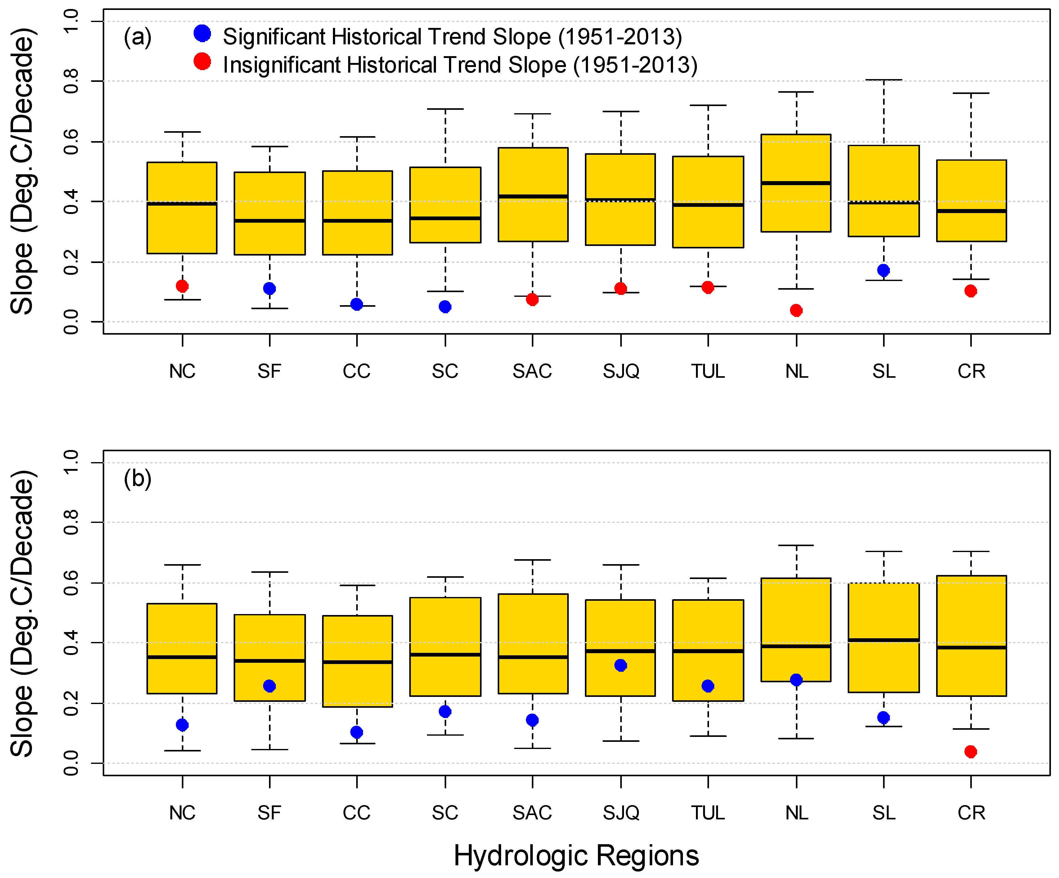
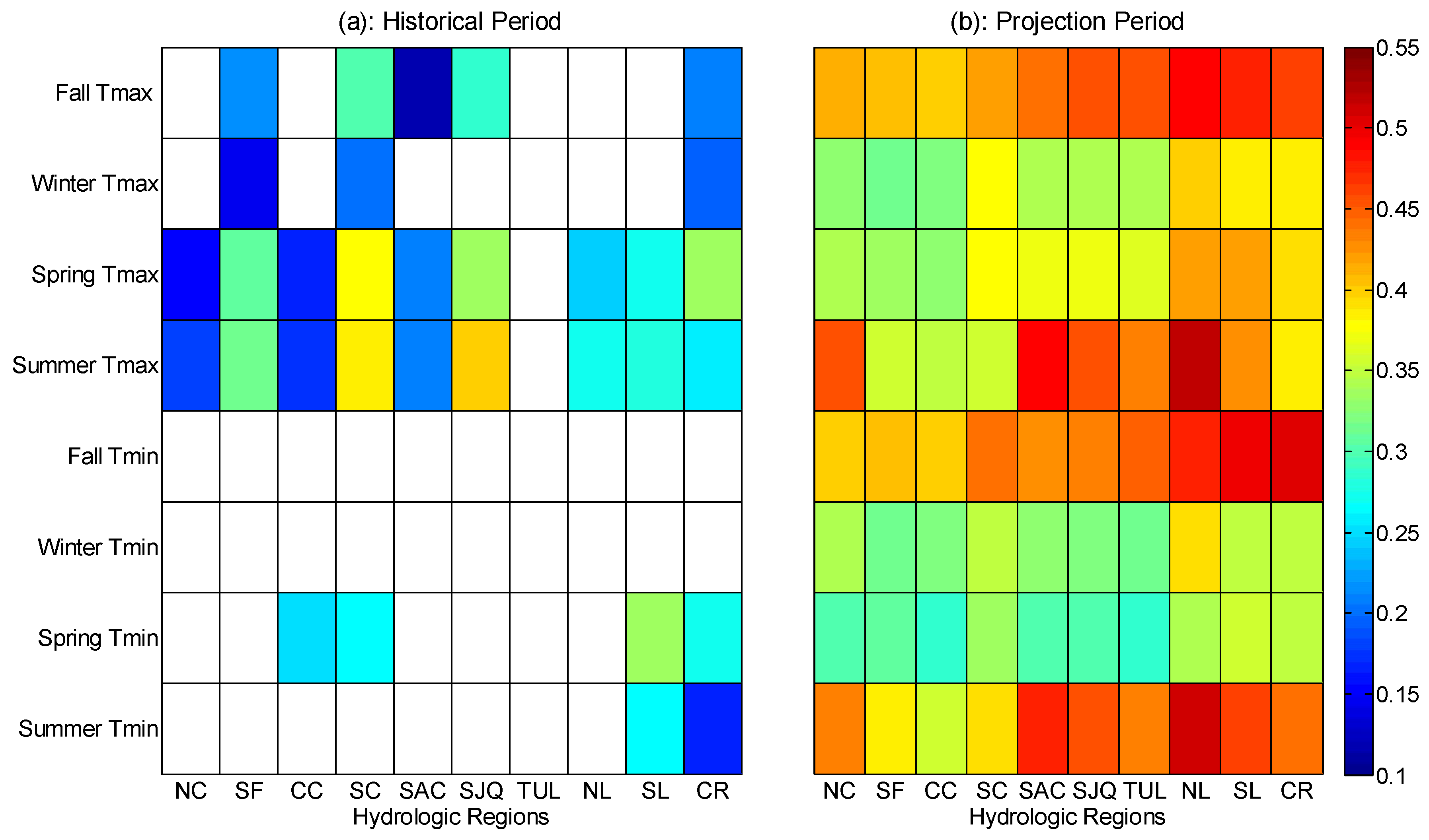
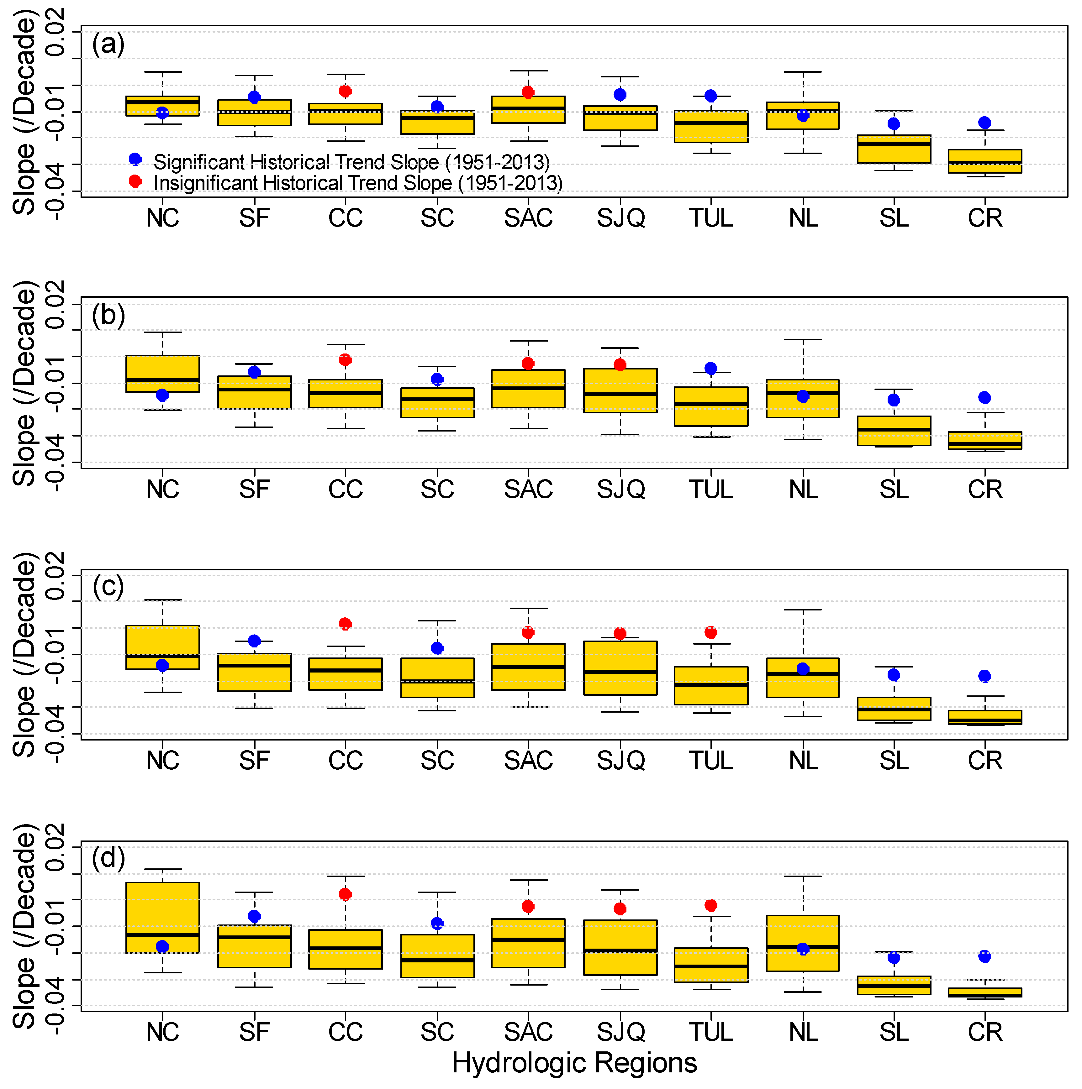
No significant trends are detected in historical annual and wet season precipitation for any study regions. Similar findings have also been reported in relevant previous studies [14]. During the projection period (2020–2099), a limited amount (no more than 15%) of model projections show significant trends (Table 5). For annual precipitation, only one projection (out of 20) has statistically significant trend for Sacramento River, South Coast, and Tulare Lake regions; three projections indicate significant trends in Central Coast and North Lahontan regions; for other regions, only two projections show significant trends. The slopes of those significant trends are all positive.
For wet season precipitation, no projections show any significant trends for the driest two regions (Colorado River and South Lahontan). For San Francisco Bay, Central Coast, South Coast, San Joaquin River, Tulare Lake, and North Lahontan regions, the projections showing significant trends are exactly the same as those showing significant trends in annual precipitation. For the two wettest regions (North Coast and Sacramento River), three projections show significant changes. Different from annual precipitation, two projections on wet season precipitation (one for Central Coast region and the other for Sacramento River region) exhibit a decreasing tendency. Nevertheless, similar to the annual precipitation, no significant changes are expected in the majority of climate model projections on wet season precipitation through 2099.

3.2.2. Temperature

All 20 projections on mean annual maximum temperature (Figure 9a) and minimum temperature (Figure 9b) show significant increasing trends. On average, the increasing rates of the Central Valley regions (SAC, SJQ, and TUL) are fairly close to each other. The increasing rates of the coast regions (NC, SF, CC, and SC) and eastern regions (NL, SL, and CR) are slightly smaller and higher, respectively, compared to that of the Central Valley regions. Particularly, the median increasing rate in the coolest region, North Lahontan, is the highest among all regions in maximum temperature. This is mostly in line with what Figure 5 and Figure 6 illustrate. In the historical period, both variables also exhibit increasing trends. However, for maximum temperature, only the trends for Central Coast, South Coast, San Francisco Bay, and South Lahontan regions are statistically significant at a significance level of 0.05. For minimum temperature, the trends of all regions except for Colorado River region are significant. Compared to historical trends, most projected trends have higher increasing rates. In general, the increasing trend is more significant in maximum temperature than in minimum temperature, implying that temperature range (difference between maximum and minimum temperature) is likely to increase. Comparing different regions, on average, the coastal regions (NC, SF, CC, and SC) tend to have the relatively smaller increasing rates while the eastern regions generally have the highest increasing rates. This is generally consistent with what has been observed in Figure 6.
Similar to those observed on the annual scale (Figure 9), not all regions have significant trends in historical maximum temperature and minimum temperature on the seasonal scale (Figure 10a). Specifically, fall and winter minimum temperature exhibits no statistically significant changes for any region. Furthermore, the Tulare Lake region does not observe any significant trends in its maximum or minimum temperature in any season. Comparing two temperature variables, maximum temperature shows significant increasing trend in most cases while minimum temperature only exhibits significant warming in a couple of seasons (spring and summer) for a few regions. In contrast, mean projections on seasonal maximum temperature and minimum temperature show significant warming trends consistently for all regions (Figure 10b). Warming in summer and fall is more pronounced than warming in two other seasons. Looking at different regions, the eastern regions generally have the highest increasing trend while the coastal regions have the smallest amount of increasing rate. Particularly, the coolest region, North Lahontan, has the most significant increasing tendency in both maximum temperature and minimum temperature. The region has the highest seasonal warming rate in both maximum temperature (0.52 °C/decade) and minimum temperature (0.51 °C/decade) in summer. Those observations are largely in line with what Figure 7 shows.

3.2.3. Drought Index

California is prone to drought, with examples being the 1976–1977, 1988–1992, 2007–2009, and 2012–2013 droughts [80]. While the occurrence and lasting period of drought events are difficult to predict decades in advance, the overall tendency (i.e., trend) of drought events can shed light on long-term drought response planning activities. This section looks at projected future drought conditions (represented by the SPEI index) at one- to four-year temporal scales which are relevant to our operational planning practices. Figure 11 shows trend slopes of SPEI-12, SPEI-24, SPEI-36, and SPEI-48 calculated from projected precipitation and temperature data, along with their counterparts in the historical period. On average, all regions are expecting a decreasing trend (negative slope value). This is particularly true for dry regions including the Colorado River, South Lahontan, and Tulare Lake. All 20 projections have a decreasing tendency consistently, indicating more severe droughts for those regions on the annual, two-year, three-year, and four-year scales. For other regions, there is no such consensus. However, the majority of projections show a decreasing trend. It should be highlighted that, for the wettest region, North Coast, most projections have a relatively milder decreasing trend compared to the historical baseline. This suggests that projected increase in precipitation over this region outweighs the effect of warming. For the coolest region, North Lahontan, the median trend slopes of projected SPEI values are generally around the historical trend slope values. This implies that projected precipitation increase in this region offsets the impact of warming. For other regions, most projections have a steeper decreasing trend compared to their historical counterparts, indicating that projected increases in precipitation are not sufficient to offset the effect of warming. Particularly, for the driest region, Colorado River, the decreasing rates of all 20 projections are higher than its baseline counterpart. This suggests that this region is the least resilient to warming and thus most prone to aridity (as represented by SPEI index) among all study regions.
It is worth noting that not all trends identified in the historical and projection periods are statistically significant at a significance level of 0.05. The Central Coast region and Sacramento River region show no significant changes in SPEI values (Figure 11). Additionally, on three-year scale and four-year scale, all Central Valley regions (SAC, SJQ, and TUL) have no increasing or decreasing tendency in drought represented by SPEI during the historical period. In the projection period (Table 6), for the driest two regions, Colorado River and South Lahontan, all 20 projections show consistently significant trend in SPEI at the four time scales considered. This is no such consensus for other regions. However, the majority of projections still show significant trends. For instance, only one out of 20 (5%) projections exhibit insignificant changes in Tulare Lake region. For another relatively dry region, South Coast, all projections show significant trends in SPEI on the three-year scale (SPEI-36) and four-year scale (SPEI-48) while only one projection (5%) has insignificant trend on the annual scale (SPEI-12) and two-year scale (SPEI-24). The wettest region, North Coast, has the highest amount (25% to 30%) of projections that show no significant trend. For the second wettest region, Sacramento River, 15–20% of the projections indicate no significant trend. Overall, those projections agree more with each other on the increasing aridity in dry regions than in wet regions irrespective of the time scales investigated.

4. Discussion and Conclusions

This study investigated potential changes in future precipitation, temperature, and drought (as represented by SPEI) across 10 hydrologic regions defined by the California Department of Water Resources. The latest climate model projections on these variables through 2099 representing the state of the current climate science were applied for this purpose. Changes were explored in terms of differences from a historical baseline as well as the changing trend.
Results indicate that warming is expected across all regions in all temperature projections, particularly in late-century. There is no such consensus in precipitation, with projections ranging mostly from −25% to +50% different from the historical baseline. There is no statistically significant increasing or decreasing trend in historical precipitation as well as in the majority of the projections. However, on average, precipitation is expected to increase slightly for most regions. It should be noted that this finding is not completely in line with a previous study that indicates decreases in future California precipitation [81]. The major difference stems from the fact that different sets of data are applied in the two studies. Specifically, the current study focused on precipitation and temperature projections from 10 GCMs models (versus 42 models used by the previous study) that are deemed most appropriate for water resources planning studies in California. Compared to wet regions, dry regions are projected to have more severe drought conditions represented by SPEI. Those findings are generally consistent with what have been reported in previous studies [21,26,28,76]. A new finding of this study is that the coolest region, North Lahontan, tends to have the highest increases in both minimum and maximum temperature and a significant amount of increase in wet season precipitation, indicative of naturally increasing flood risk in this region. In another new finding, the warming in summer and fall (when water demand is typically high and precipitation is limited) is expected to be more significant than the warming in winter and spring
In general, the findings of this study are meaningful from both scientific and practical perspectives. From a scientific point of view, these findings provide useful information that can be utilized to improve the current flood and water supply forecasting models. For instance, the coolest region, North Lahontan, is expecting the most significant warming as well as increases in wet season precipitation. This region is largely impacted by snow because of its high elevation. These expected changes will most likely intensify regional rainfall (more precipitation comes as rainfall as warming elevates the snowline) and spring snowmelt, increasing flood risks in the future. This region needs to be closely monitored in the future, particularly near and above the current snowline. The current flood forecasting model uses a parameter to cap the maximum possible snowmelt rate [82]. To reflect the expected warming, this parameter needs to be increased accordingly to better model snowmelt. Taking one step further, the snow accumulation and snowmelt processes based on which the current forecasting model is developed are derived under the stationary assumption. In a non-stationary environment, these processes need to be revisited and updated accordingly as relevant new observations become available. Additionally, the current snowmelt model is temperature-index based. Snowmelt is a thermodynamic process driven more by radiation than temperature. Development and implementation of radiation-driven snowmelt model in operations are ongoing and will be reported in our future work.
From a practical standpoint, these findings can help inform water managers in making adaptive management plans. For instance, vulnerability assessment is typically the first step in developing any mitigation and adaptation strategies [83]. Corresponding adaptation strategies such as supply diversification or increased volume management capacity should be tailored for the characteristics of the regions and their particular impacts to a changing climate. All in all, this study has the potential to help decision-makers move from a reactive position of responding to hydroclimatic events as they happen to a pro-active position with region-specific strategies for improved water resources management in the future. These strategies facilitate improving the resilience of California’s physical water framework and the preparedness of its institutional framework via investments (e.g., where, when, on what, and how much) in advance.
Despite its scientific and practical significance in guiding long-term strategical water resources planning, the study addressed temperature and precipitation changes at annual and seasonal scales at the hydrologic region scale. For time-sensitive and localized activities including emergency response and management, those changes at a finer temporal and spatial scale at which extreme events occur need to be explored. Extreme climatic indices (e.g., daily maximum precipitation, heat wave, etc.) with daily resolution at the watershed scale have been extracted from the 20 climate projections applied in this study. They will be analyzed and presented in a follow-up study. Furthermore, as opposed to precipitation and temperature, streamflow runoff is normally the variable directly used to inform real-time decision making (e.g., determination of reservoir release schedule). Those climate projections have been used as input to drive a distributed hydrologic model, the Variable Infiltration Capability model, to produce daily inflow projections through 2099 for major water supply reservoirs in California. Those flow data will be analyzed in terms of volume, variability, and frequency and reported in a companion study.

Acknowledgments

The authors would like to thank four anonymous reviewers for their valuable comments that largely helped improve the quality of this study. The authors would also like to thank their colleague Mahesh Gatuam and Jianzhong Wang for discussions on previous studies leading to the current work. Technical editing from Charlie Olivares is acknowledged. The authors also want to thank John Andrew, Prabhjot (Nicky) Sandhu, and Jamie Anderson for their management support on the study. Any findings, opinions, and conclusions expressed in this paper are solely the authors’ and do not reflect the views or opinions of their employer.

Author Contributions

The study was conceived by the authors together. M.H. conducted the study and wrote the paper. A.S., E.L. and M.A. provided critical discussions.

Conflicts of Interest

The authors declare no conflict of interest.

References

  1. Jones, J. California, a state of extremes: Management framework for present-day and future hydroclimate extremes. In Water Policy and Planning in a Variable and Changing Climate; Miller, K., Hamlet, A.F., Kenney, D.S., Redmond, K.T., Eds.; Taylor & Francis Group: Boca Raton, FL, USA, 2016; pp. 207–222. [Google Scholar]
  2. Dettinger, M.D.; Ralph, F.M.; Das, T.; Neiman, P.J.; Cayan, D.R. Atmospheric rivers, floods and the water resources of California. Water 2011, 3, 445–478. [Google Scholar] [CrossRef]
  3. U.S. Census Bureau. 2010 Census Summary File 1. Available online: https://www.census.gov/2010census/data/ (accessed on 1 August 2010).
  4. Lund, J.R. Flood management in California. Water 2012, 4, 157–169. [Google Scholar] [CrossRef]
  5. California Department of Water Resources. California Water Plan Update 2013; California Department of Water Resources: Sacramento, CA, USA, 2014.
  6. Chung, F.; Kelly, K.; Guivetchi, K. Averting a California water crisis. J. Water Resour. Plan. Manag. 2002, 128, 237–239. [Google Scholar] [CrossRef]
  7. Anderson, J.; Chung, F.; Anderson, M.; Brekke, L.; Easton, D.; Ejeta, M.; Peterson, R.; Snyder, R. Progress on incorporating climate change into management of California’s water resources. Clim. Chang. 2008, 87, 91–108. [Google Scholar] [CrossRef]
  8. Kapnick, S.; Hall, A. Observed climate–snowpack relationships in California and their implications for the future. J. Clim. 2010, 23, 3446–3456. [Google Scholar] [CrossRef]
  9. McCabe, G.J.; Clark, M.P. Trends and variability in snowmelt runoff in the western United States. J. Hydrometeorol. 2005, 6, 476–482. [Google Scholar] [CrossRef]
  10. Mote, P.W. Trends in snow water equivalent in the Pacific Northwest and their climatic causes. Geophys. Res. Lett. 2003, 30. [Google Scholar] [CrossRef]
  11. Mote, P.W.; Hamlet, A.F.; Clark, M.P.; Lettenmaier, D.P. Declining mountain snowpack in western North America. Bull. Am. Meteorol. Soc. 2005, 86, 39–49. [Google Scholar] [CrossRef]
  12. Stewart, I.T.; Cayan, D.R.; Dettinger, M.D. Changes in snowmelt runoff timing in western North America under a business as usual climate change scenario. Clim. Chang. 2004, 62, 217–232. [Google Scholar] [CrossRef]
  13. Regonda, S.K.; Rajagopalan, B.; Clark, M.; Pitlick, J. Seasonal cycle shifts in hydroclimatology over the western United States. J. Clim. 2005, 18, 372–384. [Google Scholar] [CrossRef]
  14. He, M.; Gautam, M. Variability and trends in precipitation, temperature and drought indices in the State of California. Hydrology 2016, 3, 14. [Google Scholar] [CrossRef]
  15. He, M.; Russo, M.; Anderson, M. Predictability of seasonal streamflow in a changing climate in the Sierra Nevada. Climate 2016, 4, 57. [Google Scholar] [CrossRef]
  16. He, M.; Russo, M.; Anderson, M.; Fickenscher, P.; Whitin, B.; Schwarz, A.; Lynn, E. Changes in extremes of temperature, precipitation, and runoff in California’s Central Valley during 1949–2010. Hydrology 2017, 5, 1. [Google Scholar] [CrossRef]
  17. Hatchett, B.J.; Daudert, B.; Garner, C.B.; Oakley, N.S.; Putnam, A.E.; White, A.B. Winter snow level rise in the northern Sierra Nevada from 2008 to 2017. Water 2017, 9, 899. [Google Scholar] [CrossRef]
  18. Huppert, H.E.; Sparks, R.S.J. Extreme natural hazards: Population growth, globalization and environmental change. Philos. Trans. A Math. Phys. Eng. Sci. 2006, 364, 1875–1888. [Google Scholar] [CrossRef] [PubMed]
  19. Cavallo, E.; Galiani, S.; Noy, I.; Pantano, J. Catastrophic natural disasters and economic growth. Rev. Econ. Stat. 2013, 95, 1549–1561. [Google Scholar] [CrossRef]
  20. Hanak, E.; Lund, J.R. Adapting California’s water management to climate change. Clim. Chang. 2012, 111, 17–44. [Google Scholar] [CrossRef]
  21. Dettinger, M.; Anderson, J.; Anderson, M.; Brown, L.; Cayan, D.; Maurer, E. Climate change and the Delta. San Fr. Estuary Watershed Sci. 2016, 14, 1–26. [Google Scholar] [CrossRef]
  22. Das, T.; Dettinger, M.D.; Cayan, D.R.; Hidalgo, H.G. Potential increase in floods in California’s Sierra Nevada under future climate projections. Clim. Chang. 2011, 109, 71–94. [Google Scholar] [CrossRef]
  23. Das, T.; Maurer, E.P.; Pierce, D.W.; Dettinger, M.D.; Cayan, D.R. Increases in flood magnitudes in California under warming climates. J. Hydrol. 2013, 501, 101–110. [Google Scholar] [CrossRef]
  24. Sun, F.; Hall, A.; Schwartz, M.; Walton, D.B.; Berg, N. Twenty-first-century snowfall and snowpack changes over the southern California Mountains. J. Clim. 2016, 29, 91–110. [Google Scholar] [CrossRef]
  25. Berg, N.; Hall, A. Increased interannual precipitation extremes over California under climate change. J. Clim. 2015, 28, 1–11. [Google Scholar] [CrossRef]
  26. Tebaldi, C.; Hayhoe, K.; Arblaster, J.M.; Meehl, G.A. Going to the extremes. Clim. Chang. 2006, 79, 185–211. [Google Scholar] [CrossRef]
  27. Wang, J.; Zhang, X. Downscaling and projection of winter extreme daily precipitation over North America. J. Clim. 2008, 21, 923–937. [Google Scholar] [CrossRef]
  28. Yoon, J.-H.; Wang, S.S.; Gillies, R.R.; Kravitz, B.; Hipps, L.; Rasch, P.J. Increasing water cycle extremes in California and in relation to ENSO cycle under global warming. Nat. Commun. 2015, 6, 8657. [Google Scholar] [CrossRef] [PubMed]
  29. Maurer, E.P. Uncertainty in hydrologic impacts of climate change in the Sierra Nevada, California, under two emissions scenarios. Clim. Chang. 2007, 82, 309–325. [Google Scholar] [CrossRef]
  30. Cayan, D.R.; Maurer, E.P.; Dettinger, M.D.; Tyree, M.; Hayhoe, K. Climate change scenarios for the California region. Clim. Chang. 2008, 87, 21–42. [Google Scholar] [CrossRef]
  31. Meehl, G.A.; Covey, C.; Taylor, K.E.; Delworth, T.; Stouffer, R.J.; Latif, M.; McAvaney, B.; Mitchell, J.F. The WCRP CMIP3 multimodel dataset: A new era in climate change research. Bull. Am. Meteorol. Soc. 2007, 88, 1383–1394. [Google Scholar] [CrossRef]
  32. Taylor, K.E.; Stouffer, R.J.; Meehl, G.A. An overview of CMIP5 and the experiment design. Bull. Am. Meteorol. Soc. 2012, 93, 485–498. [Google Scholar] [CrossRef]
  33. Van Vuuren, D.P.; Edmonds, J.; Kainuma, M.; Riahi, K.; Thomson, A.; Hibbard, K.; Hurtt, G.C.; Kram, T.; Krey, V.; Lamarque, J.-F. The representative concentration pathways: An overview. Clim. Chang. 2011, 109, 5. [Google Scholar] [CrossRef]
  34. Climate Change Technical Advisory Group (CCTAG). Perspectives and Guidance for Climate Change Analysis; California Department of Water Resources: Sacramento, CA, USA, 2015.
  35. Pierce, D.W.; Cayan, D.R.; Thrasher, B.L. Statistical downscaling using localized constructed analogs (LOCA). J. Hydrometeorol. 2014, 15, 2558–2585. [Google Scholar] [CrossRef]
  36. Lutz, A.F.; ter Maat, H.W.; Biemans, H.; Shrestha, A.B.; Wester, P.; Immerzeel, W.W. Selecting representative climate models for climate change impact studies: An advanced envelope-based selection approach. Int. J. Climatol. 2016, 36, 3988–4005. [Google Scholar] [CrossRef]
  37. Shrestha, N.K.; Wang, J. Modelling nitrous oxide (N2O) emission from soils using the soil and water assessment tool (SWAT). In Proceedings of the 2018 International SWAT Conference and Workshops, Chennai, India, 10–12 January 2018. [Google Scholar]
  38. California Department of Water Resources. 2017 Central Valley Flood Protection Plan Update; California Department of Water Resources: Sacramento, CA, USA, 2017.
  39. California Water Commission. Water Storage Investigation Program Technical Reference; California Water Commission: Sacramento, CA, USA, 2017.
  40. Livneh, B.; Bohn, T.J.; Pierce, D.W.; Munoz-Arriola, F.; Nijssen, B.; Vose, R.; Cayan, D.R.; Brekke, L. A spatially comprehensive, hydrometeorological data set for Mexico, the US, and southern Canada 1950–2013. Sci. Data 2015, 2, 150042. [Google Scholar] [CrossRef] [PubMed]
  41. Livneh, B.; Hoerling, M.P. The physics of drought in the US central great plains. J. Clim. 2016, 29, 6783–6804. [Google Scholar] [CrossRef]
  42. Bohn, T.J.; Vivoni, E.R. Process-based characterization of evapotranspiration sources over the North American monsoon region. Water Res. Res. 2016, 52, 358–384. [Google Scholar] [CrossRef]
  43. Barnhart, T.B.; Molotch, N.P.; Livneh, B.; Harpold, A.A.; Knowles, J.F.; Schneider, D. Snowmelt rate dictates streamflow. Geophys. Res. Lett. 2016, 43, 8006–8016. [Google Scholar] [CrossRef]
  44. Wi, S.; Ray, P.; Demaria, E.M.; Steinschneider, S.; Brown, C. A user-friendly software package for VIC hydrologic model development. Environ. Modell. Softw. 2017, 98, 35–53. [Google Scholar] [CrossRef]
  45. He, M.; Russo, M.; Anderson, M. Hydroclimatic characteristics of the 2012–2015 California drought from an operational perspective. Climate 2017, 5, 5. [Google Scholar] [CrossRef]
  46. Dai, A. Drought under global warming: A review. WIREs Clim. Chang. 2011, 2, 45–65. [Google Scholar] [CrossRef]
  47. Heim, R.R., Jr. A review of twentieth-century drought indices used in the United States. Bull. Am. Meteorol. Soc. 2002, 83, 1149–1165. [Google Scholar] [CrossRef]
  48. Keyantash, J.; Dracup, J.A. The quantification of drought: An evaluation of drought indices. Bull. Am. Meteorol. Soc. 2002, 83, 1167–1180. [Google Scholar] [CrossRef]
  49. McKee, T.B.; Doesken, N.J.; Kleist, J. The relationship of drought frequency and duration to time scales. In Proceedings of the 8th Conference on Applied Climatology, Anaheim, CA, USA, 17–22 January 1993; American Meteorological Society: Boston, MA, USA; pp. 179–183. [Google Scholar]
  50. Ciais, P.; Reichstein, M.; Viovy, N.; Granier, A.; Ogée, J.; Allard, V.; Aubinet, M.; Buchmann, N.; Bernhofer, C.; Carrara, A. Europe-wide reduction in primary productivity caused by the heat and drought in 2003. Nature 2005, 437, 529–533. [Google Scholar] [CrossRef] [PubMed]
  51. Adams, H.D.; Guardiola-Claramonte, M.; Barron-Gafford, G.A.; Villegas, J.C.; Breshears, D.D.; Zou, C.B.; Troch, P.A.; Huxman, T.E. Temperature sensitivity of drought-induced tree mortality portends increased regional die-off under global-change-type drought. Proc. Natl. Acad. Sci. USA 2009, 106, 7063–7066. [Google Scholar] [CrossRef] [PubMed]
  52. Breshears, D.D.; Cobb, N.S.; Rich, P.M.; Price, K.P.; Allen, C.D.; Balice, R.G.; Romme, W.H.; Kastens, J.H.; Floyd, M.L.; Belnap, J. Regional vegetation die-off in response to global-change-type drought. Proc. Natl. Acad. Sci. USA 2005, 102, 15144–15148. [Google Scholar] [CrossRef] [PubMed]
  53. Swain, D.L. A tale of two California droughts: Lessons amidst record warmth and dryness in a region of complex physical and human geography. Geophys. Res. Lett. 2015, 42, 9999. [Google Scholar] [CrossRef]
  54. Seager, R.; Hoerling, M.; Schubert, S.; Wang, H.; Lyon, B.; Kumar, A.; Nakamura, J.; Henderson, N. Causes of the 2011–2014 California drought. J. Clim. 2015, 28, 6997–7024. [Google Scholar] [CrossRef]
  55. Wang, S.Y.; Hipps, L.; Gillies, R.R.; Yoon, J.H. Probable causes of the abnormal ridge accompanying the 2013–2014 California drought: ENSO precursor and anthropogenic warming footprint. Geophys. Res. Lett. 2014, 41, 3220–3226. [Google Scholar] [CrossRef]
  56. Vicente-Serrano, S.M.; Beguería, S.; López-Moreno, J.I. A multiscalar drought index sensitive to global warming: The standardized precipitation evapotranspiration index. J. Clim. 2010, 23, 1696–1718. [Google Scholar] [CrossRef]
  57. Abramowitz, M.; Stegun, I.A. Handbook of mathematical functions. Appl. Math. Ser. 1966, 55, 39. [Google Scholar] [CrossRef]
  58. Beguería, S.; Vicente-Serrano, S.M.; Angulo-Martínez, M. A multiscalar global drought dataset: The speibase: A new gridded product for the analysis of drought variability and impacts. Bull. Am. Meteorol. Soc. 2010, 91, 1351–1356. [Google Scholar] [CrossRef]
  59. Vicente-Serrano, S.M.; Beguería, S.; López-Moreno, J.I.; Angulo, M.; El Kenawy, A. A new global 0.5 gridded dataset (1901–2006) of a multiscalar drought index: Comparison with current drought index datasets based on the Palmer drought severity index. J. Hydrometeorol. 2010, 11, 1033–1043. [Google Scholar] [CrossRef]
  60. Vicente-Serrano, S.M.; Van der Schrier, G.; Beguería, S.; Azorin-Molina, C.; Lopez-Moreno, J.-I. Contribution of precipitation and reference evapotranspiration to drought indices under different climates. J. Hydrol. 2015, 526, 42–54. [Google Scholar] [CrossRef]
  61. Li, W.; Hou, M.; Chen, H.; Chen, X. Study on drought trend in south China based on standardized precipitation evapotranspiration index. J. Nat. Disasters 2012, 21, 84–90. [Google Scholar]
  62. Beguería, S.; Vicente-Serrano, S.M.; Reig, F.; Latorre, B. Standardized precipitation evapotranspiration index (SPEI) revisited: Parameter fitting, evapotranspiration models, tools, datasets and drought monitoring. Int. J. Climatol. 2014, 34, 3001–3023. [Google Scholar] [CrossRef]
  63. Banimahd, S.A.; Khalili, D. Factors influencing markov chains predictability characteristics, utilizing SPI, RDI, EDI and SPEI drought indices in different climatic zones. Water Resour. Manag. 2013, 27, 3911–3928. [Google Scholar] [CrossRef]
  64. Thornthwaite, C.W. An approach toward a rational classification of climate. Geogr. Rev. 1948, 38, 55–94. [Google Scholar] [CrossRef]
  65. Helsel, D.R.; Hirsch, R.M. Statistical Methods in Water Resources; Elsevier: New York, NY, USA, 1992; Volume 49. [Google Scholar]
  66. Hirsch, R.M.; Helsel, D.; Cohn, T.; Gilroy, E. Statistical analysis of hydrologic data. Handb. Hydrol. 1993, 17, 11–55. [Google Scholar]
  67. Mann, H. Non-parametric tests against trend. Econometrica 1945, 13, 245–259. [Google Scholar] [CrossRef]
  68. Kendall, M.G. Rank Correlation Methods; Charles Griffin: London, UK, 1975. [Google Scholar]
  69. Yue, S.; Pilon, P.; Cavadias, G. Power of the Mann–Kendall and Spearman’s rho tests for detecting monotonic trends in hydrological series. J. Hydrol. 2002, 259, 254–271. [Google Scholar] [CrossRef]
  70. Yue, S.; Pilon, P.; Phinney, B.; Cavadias, G. The influence of autocorrelation on the ability to detect trend in hydrological series. Hydrol. Process. 2002, 16, 1807–1829. [Google Scholar] [CrossRef]
  71. Thiel, H. A rank-invariant method of linear and polynomial regression analysis, part 3. In Proceedings of Koninalijke Nederlandse Akademie van Weinenschatpen A; Royal Netherlands Academy of Arts and Sciences: Amsterdam, The Netherlands, 1950; pp. 1397–1412. [Google Scholar]
  72. Sen, P.K. Estimates of the regression coefficient based on Kendall’s tau. J. Am. Stat. Assoc. 1968, 63, 1379–1389. [Google Scholar] [CrossRef]
  73. Adams, D.K.; Comrie, A.C. The North American monsoon. Bull. Am. Meteorol. Soc. 1997, 78, 2197–2213. [Google Scholar] [CrossRef]
  74. Higgins, R.; Yao, Y.; Wang, X. Influence of the North American monsoon system on the US summer precipitation regime. J. Clim. 1997, 10, 2600–2622. [Google Scholar] [CrossRef]
  75. Gutzler, D.S.; Robbins, T.O. Climate variability and projected change in the western United States: Regional downscaling and drought statistics. Clim. Dyn. 2011, 37, 835–849. [Google Scholar] [CrossRef]
  76. Dettinger, M.D. Projections and downscaling of 21st century temperatures, precipitation, radiative fluxes and winds for the southwestern US, with focus on Lake Tahoe. Clim. Chang. 2013, 116, 17–33. [Google Scholar] [CrossRef]
  77. Elguindi, N.; Grundstein, A. An integrated approach to assessing 21st century climate change over the contiguous US using the NARCCAP RCM output. Clim. Chang. 2013, 117, 809–827. [Google Scholar] [CrossRef]
  78. Scherer, M.; Diffenbaugh, N.S. Transient twenty-first century changes in daily-scale temperature extremes in the United States. Clim. Dyn. 2014, 42, 1383–1404. [Google Scholar] [CrossRef]
  79. Ashfaq, M.; Bowling, L.C.; Cherkauer, K.; Pal, J.S.; Diffenbaugh, N.S. Influence of climate model biases and daily-scale temperature and precipitation events on hydrological impacts assessment: A case study of the United States. J. Geophys. Res. Atmos. 2010, 115. [Google Scholar] [CrossRef]
  80. California Department of Water Resources. California’s Most Significant Droughts: Comparing Historical and Recent Conditions; California Department of Water Resources: Sacramento, CA, USA, 2015; p. 136.
  81. Kirtman, B.; Power, S.; Adedoyin, A.; Boer, G.; Bojariu, R.; Camilloni, I.; Doblas-Reyes, F.; Fiore, A.; Kimoto, M.; Meehl, G. Chapter 11—Near-term climate change: Projections and predictability. In Climate Change 2013: The Physical Science Basis. IPCC Working Group I Contribution to Ar5; IPCC, Ed.; Cambridge University Press: Cambridge, UK, 2013. [Google Scholar]
  82. Anderson, E.A. National Weather Service River Forecast System—sNow Accumulation and Ablation Model; Technical Memorandum NWS HYDRO-17; NOAA: Silver Spring, MD, USA, 1973.
  83. Andrew, J.T.; Sauquet, E. Climate change impacts and water management adaptation in two mediterranean-climate watersheds: Learning from the Durance and Sacramento rivers. Water 2016, 9, 126. [Google Scholar] [CrossRef]
Figure 1. Ten hydrologic regions in California: North Coast (NC), San Francisco Bay (SF), Central Coast (CC), South Coast (SC), Sacramento River (SAC), San Joaquin River (SJQ), Tulare Lake (TUL), North Lahontan (NL), South Lahontan (SL), and Colorado River (CR). Dots represent the centroid points of individual climate projection grids (1/16th degree) located in each region.
Climate 06 00031 g001
Figure 2. Long-term (1951–2013) mean monthly precipitation (a) and temperature (b) of 10 hydrologic regions.
Climate 06 00031 g002
Figure 3. SPEI-12 of: (a) San Francisco Bay region; (b) Sacramento River region; and (c) Colorado River region during the historical period (1951–2013). Blue color indicates wet conditions; red color designates drought conditions. The purple line is the threshold below which extreme drought conditions exist.
Climate 06 00031 g003
Figure 4. Percent differences (%) between historical and mean RCP 4.5 projections on: (a) annual precipitation in mid- century; (b) wet season precipitation in mid-century; (c) annual precipitation in late-century; and (d) wet season precipitation in late-century.
Climate 06 00031 g004
Figure 5. Box-and-whisker plots of percent differences (%) between historical and individual projections on: (a) annual precipitation; and (b) wet season precipitation. Yellow boxes represent mid-century results and orange boxes show late-century results.
Climate 06 00031 g005
Figure 6. Differences (°C) between historical and mean RCP 4.5 projections on mean annual: (a) maximum temperature in mid-century; (b) minimum temperature in mid-century; (c) maximum temperature in late-century; and (d) minimum temperature in late-century.
Climate 06 00031 g006
Figure 7. Box-and-whisker plots of differences (°C) between historical and individual projections on mean annual: (a) maximum temperature; and (b) minimum temperature. Yellow boxes represent mid-century results and orange boxes show late-century results.
Climate 06 00031 g007
Figure 8. Differences (°C) between historical and mean (of all 20) projections on seasonal maximum temperature (Tmax) and minimum temperature (Tmin) in: (a) mid-century; and (b) late-century.
Climate 06 00031 g008
Figure 9. Box-and-whisker plots of trend slopes of historical (1951–2013) and projected (2020–2099) mean annual: (a) maximum temperature (Tmax); and (b) minimum temperature (Tmin) (at significance level 0.05).
Climate 06 00031 g009
Figure 10. Trend slopes of (a) historical (1951–2013) and (b) projected (2020–2099) mean seasonal maximum temperature (Tmax) and minimum temperature (Tmin) (at significance level 0.05). Different colors mean different trend slopes (per decade). White color indicates no significant trends.
Climate 06 00031 g010
Figure 11. Box-and-whisker plots of significant trend slopes of: (a) SPEI-12; (b) SPEI-24; (c) SPEI-36; and (d) SPEI-48 during projection period (2020–2099) (at significance level 0.05). The slope information in historical period (1951–2013) is also shown.
Climate 06 00031 g011
Table 1. Geographic and climatic characteristics of study hydrologic regions.
IDRegion NameArea (km2)Annual Precipitation (mm)Annual Mean Temperature (°C)Population (as of 2010; Million)
NCNorth Coast49,85913909.30.81
SFSan Francisco Bay11,53564114.36.35
CCCentral Coast28,99550413.01.53
SCSouth Coast27,96845915.619.58
SACSacramento River69,75092511.42.98
SJQSan Joaquin River38,94868012.82.10
TULTulare Lake43,60440813.92.27
NLNorth Lahontan15,6725426.40.11
SLSouth Lahontan68,43419115.20.93
CRColorado River51,10312720.20.75
Table 2. GCMs Selected for California Water Resources Planning 1.
Model IDModel NameModel Institution
1ACCESS-1.0Commonwealth Scientific and Industrial Research Organisation (CSIRO) and Bureau of Meteorology (BOM), Australia
2CCSM4National Center for Atmospheric Research
3CESM1-BGCNational Science Foundation, Department of Energy, National Center for Atmospheric Research
4CMCC-CMSCentro Euro-Mediterraneo sui Cambiamenti Climatici
5CNRM-CM5Centre National de Recherches Météorologiques/Centre Européen de Recherche et de Formation Avancée en Calcul Scientifique
6CanESM2Canadian Centre for Climate Modeling and Analysis
7GFDL-CM3Geophysical Fluid Dynamics Laboratory
8HadGEM2-CCMet Office Hadley Centre
9HadGEM2-ESMet Office Hadley Centre/Instituto Nacional de Pesquisas Espaciais
10MIROC5Atmosphere and Ocean Research Institute (The University of Tokyo), National Institute for Environmental Studies, and Japan Agency for Marine-Earth Science and Technology
1 Adapted from Table 2, Table 3 and Table 4 of [34].
Table 3. Percent differences (%) between historical and mean RCP 8.5 projections on annual precipitation and wet season precipitation.
IDRegion NameAnnual Precipitation (%)Wet Season Precipitation (%)
Mid-CenturyLate-CenturyMid-CenturyLate-Century
NCNorth Coast4.45.28.410.6
SFSan Francisco Bay10.314.412.718.7
CCCentral Coast7.412.89.616.0
SCSouth Coast−0.11.41.43.9
SACSacramento River7.69.011.414.2
SJQSan Joaquin River5.47.48.011.3
TULTulare Lake0.52.72.95.8
NLNorth Lahontan6.610.311.816.9
SLSouth Lahontan−0.52.43.87.7
CRColorado River−2.3−1.54.75.9
Table 4. Differences (°C) between historical and mean RCP 8.5 projections on annual maximum and minimum temperature.
Annual Tmax (°C)Annual Tmin (°C)
Mid-CenturyLate-CenturyMid-CenturyLate-Century
NCNorth Coast2.74.32.54.1
SFSan Francisco Bay2.43.82.54.0
CCCentral Coast2.53.92.43.8
SCSouth Coast3.04.52.94.5
SACSacramento River3.04.72.74.4
SJQSan Joaquin River3.04.62.84.5
TULTulare Lake3.04.62.54.2
NLNorth Lahontan3.45.33.25.0
SLSouth Lahontan3.35.13.04.8
CRColorado River3.24.93.04.9
Table 5. Trend information of projected precipitation.
IDRegion NameNumber (Percent) of Projections with Significant Trend 1Range of Significant Trend Slope (mm/Year)
Annual Precipitation Wet Season Precipitation
NCNorth Coast2 (10%)3 (15%)3.9~5.4
SFSan Francisco Bay2 (10%)2 (10%)3.2~4.6
CCCentral Coast3 (15%)3 (15%)−0.5~3.4
SCSouth Coast1 (5%)1 (5%)2.1~2.7
SACSacramento River1 (5%)3 (15%)−2.2~6.0
SJQSan Joaquin River2 (10%)2 (10%)2.8~5.0
TULTulare Lake2 (10%)2 (10%)1.7~3.2
NLNorth Lahontan3 (15%)3 (15%)1.2~5.3
SLSouth Lahontan2 (10%)0 (0%)0.8~1.9
CRColorado River1 (5%)0 (0%)1.1
1 Significance level 0.05.
Table 6. Number (percent) of SPEI projections with insignificant trend 1 in the projection period.
IDRegion NameSPEI-12SPEI-24SPEI-36SPEI-48
NCNorth Coast6 (30%)5 (25%)5 (25%)6 (30%)
SFSan Francisco Bay5 (25%)5 (25%)5 (25%)3 (15%)
CCCentral Coast3 (15%)3 (15%)3 (15%)2 (10%)
SCSouth Coast1 (5%)1 (5%)0 (0%)0 (0%)
SACSacramento River4 (20%)3 (15%)4 (20%)3 (15%)
SJQSan Joaquin River3 (15%)2 (10%)2 (10%)2 (10%)
TULTulare Lake1 (5%)1 (5%)1 (5%)1 (5%)
NLNorth Lahontan2 (10%)3 (15%)3 (15%)0 (0%)
SLSouth Lahontan0 (0%)0 (0%)0 (0%)0 (0%)
CRColorado River0 (0%)0 (0%)0 (0%)0 (0%)
1 Significance level 0.05.

