Evaluation of Statistical-Downscaling/Bias-Correction Methods to Predict Hydrologic Responses to Climate Change in the Zarrine River Basin, Iran


Abstract
1. Introduction
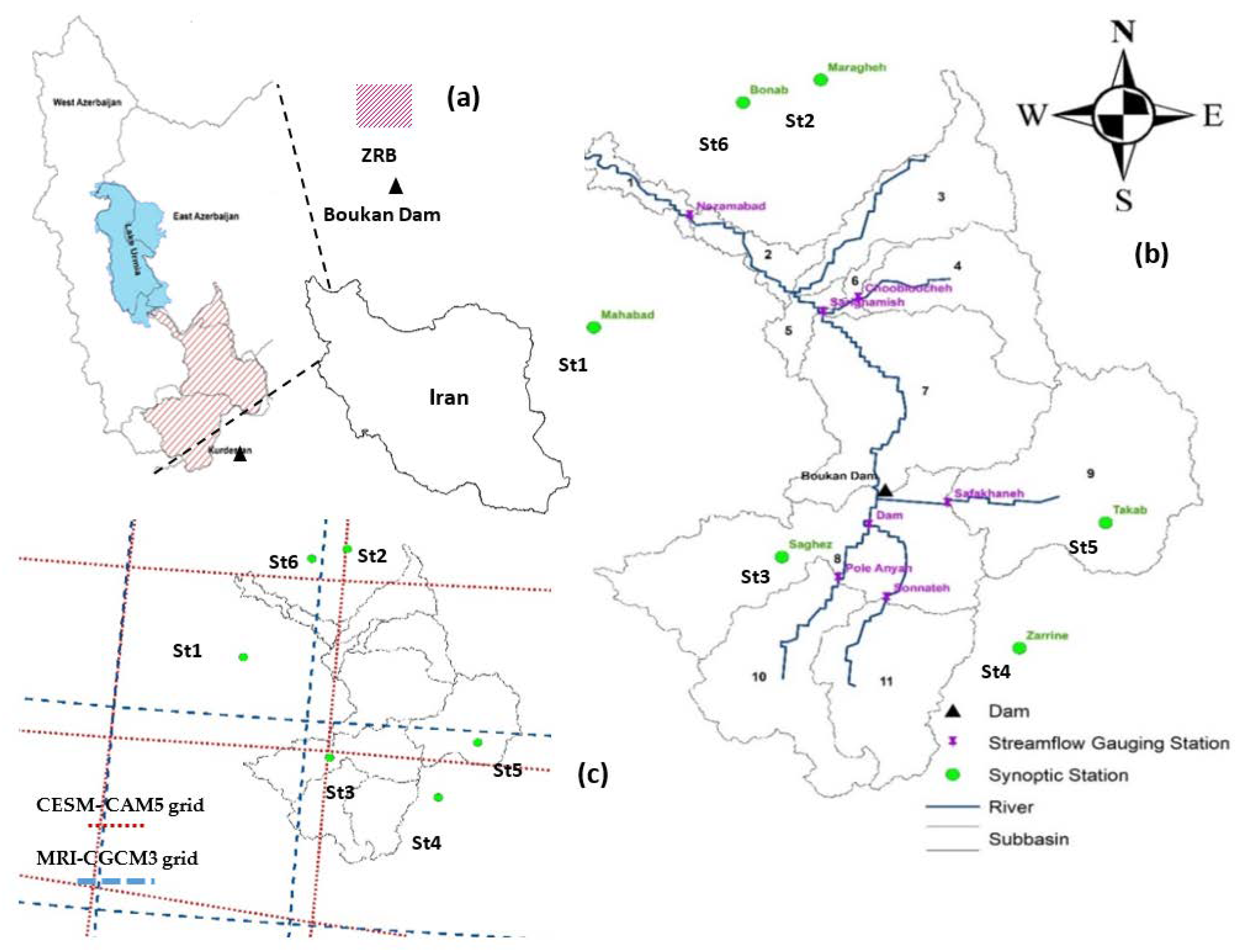
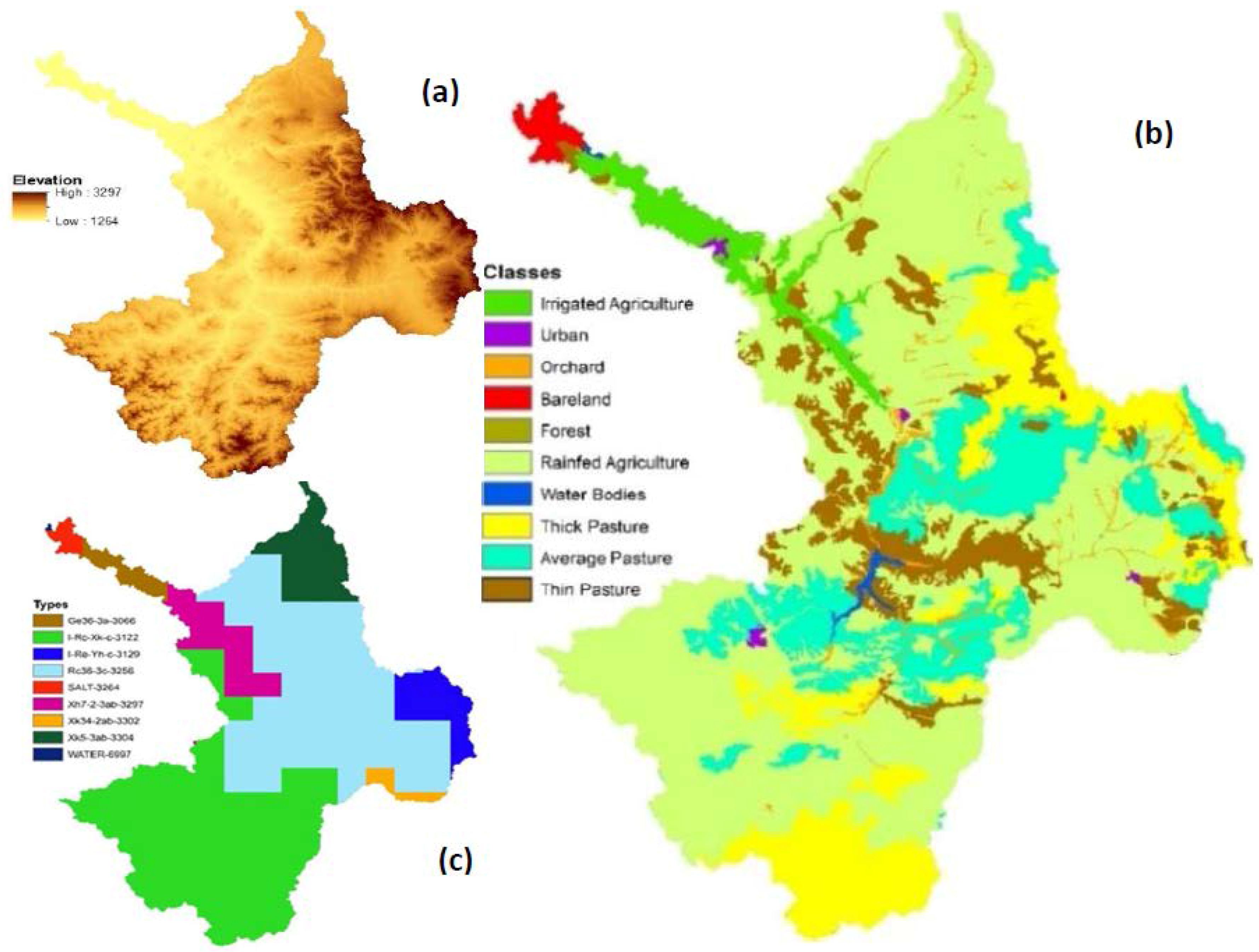
2. Study Area
3. Materials and Methods
3.1. Climate Change Scenarios and Predictions
3.1.1. Selecting the Climate Model Intercomparison Project Phase 5 (CMIP5) General Circulation Model (GCM)
3.1.2. Statistical Downscaling Model (SDSM)
3.1.3. Updated Quantile Mapping (QM) Bias Correction Technique
3.2. Integrated Hydrological Simulation Model, Soil and Water Assessment Tool (SWAT)
3.2.1. Soil and Water Assessment Tool (SWAT) Model Setup and Process Simulation
3.2.2. Calibration and Validation
3.3. Reservoir Dependable Water and Environmental Water Rights
4. Results and Discussion
4.1. SDSM Downscaling of Precipitation and Temperatures
Calibration and Validation of the SDSM Model
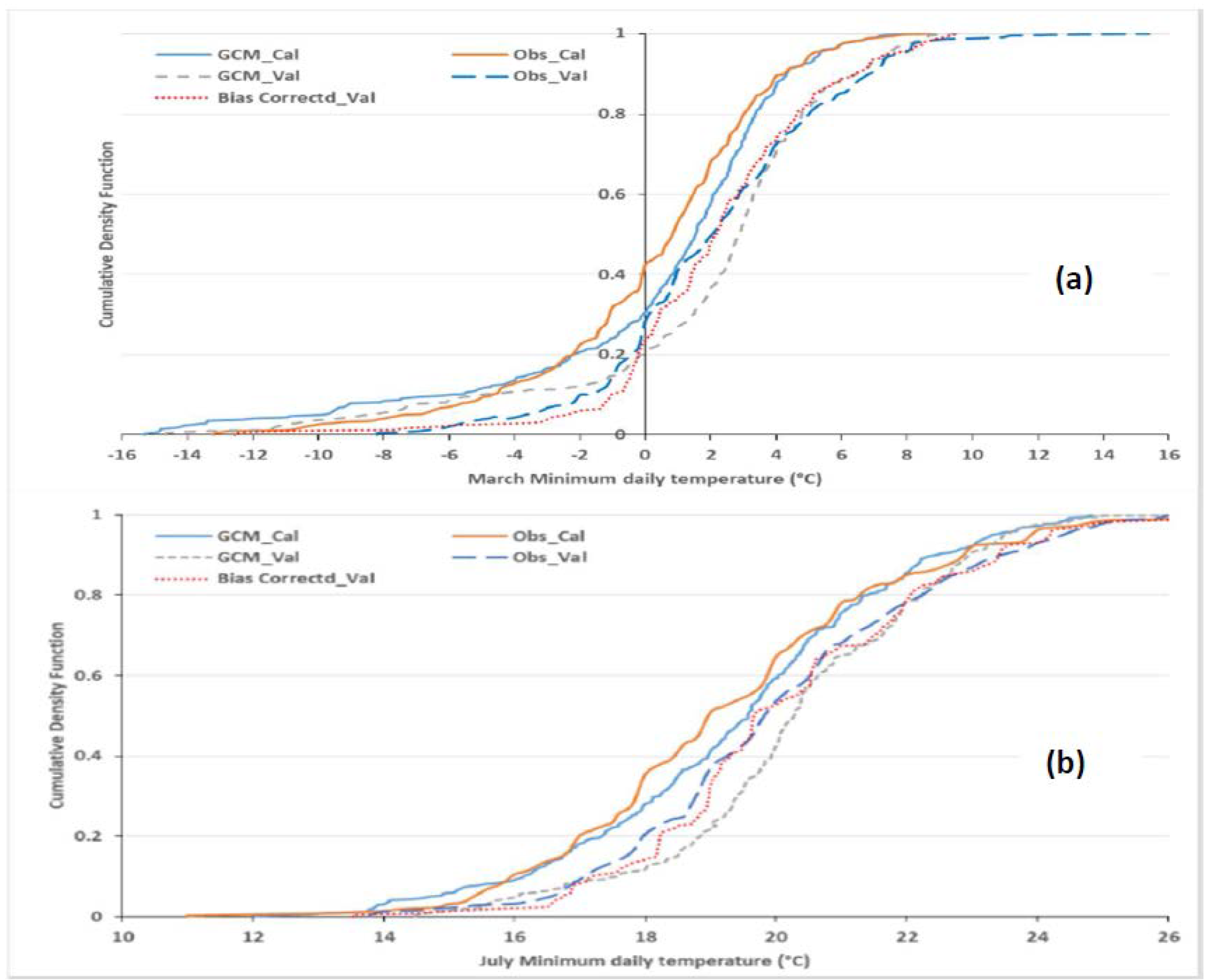
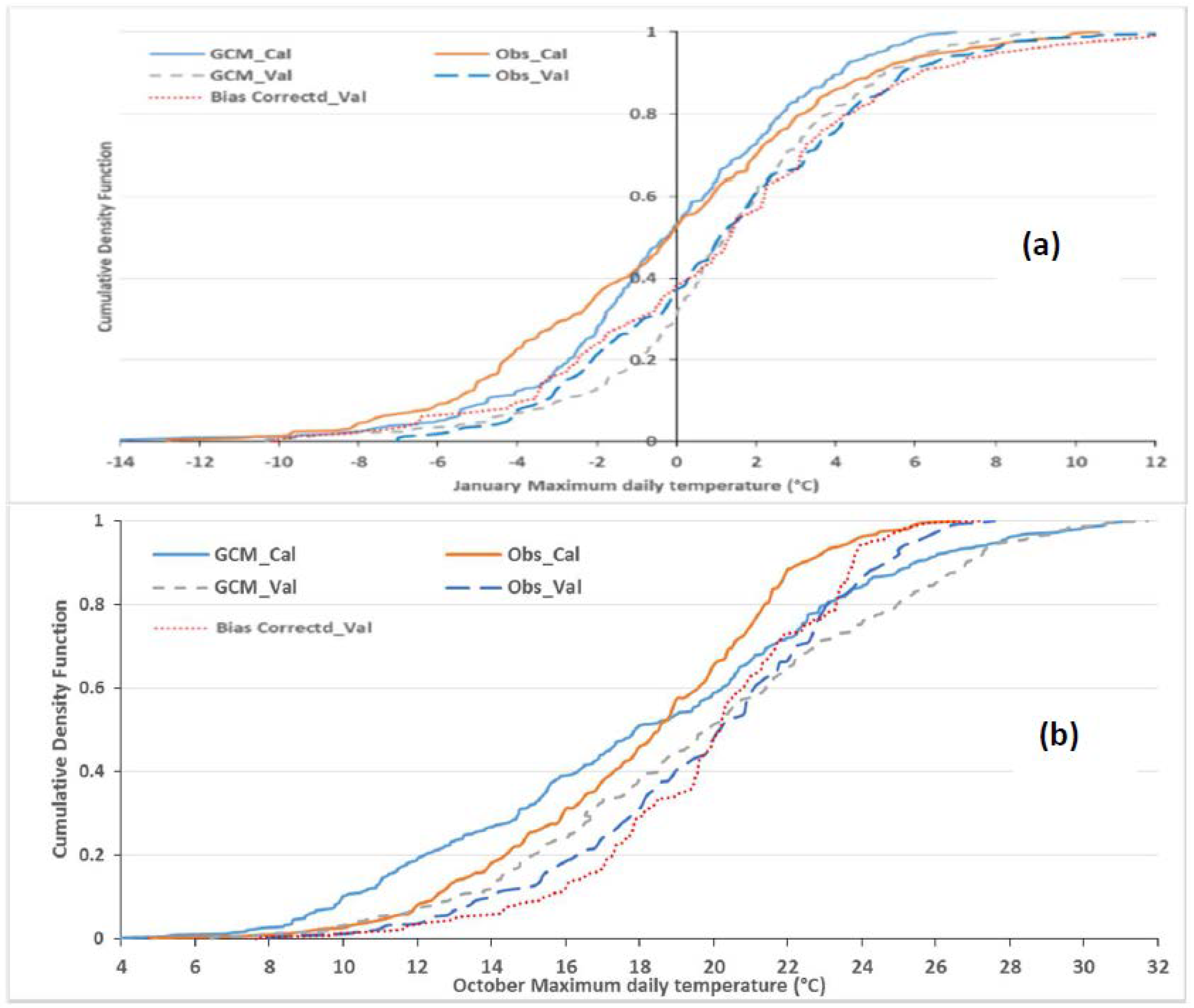
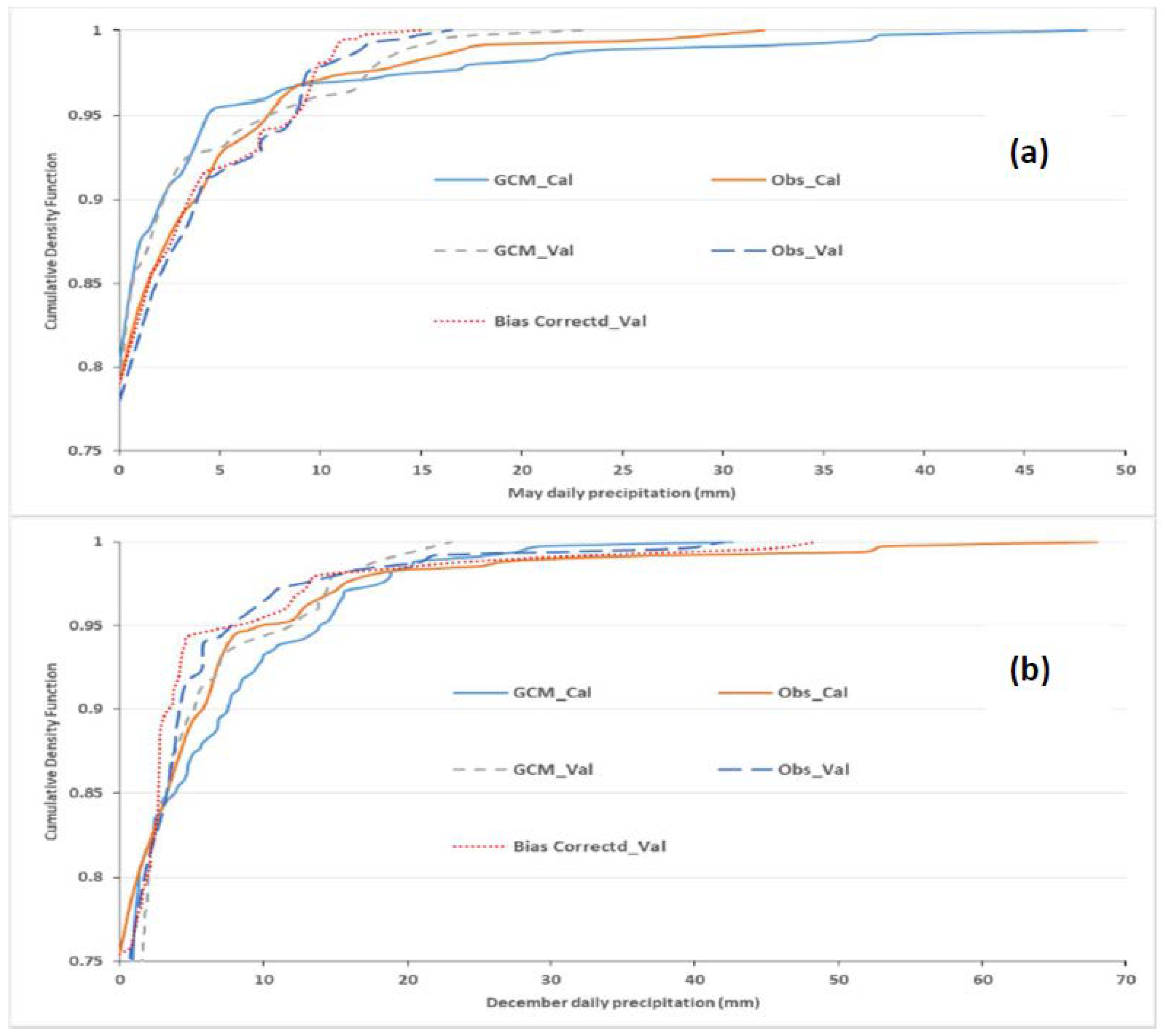
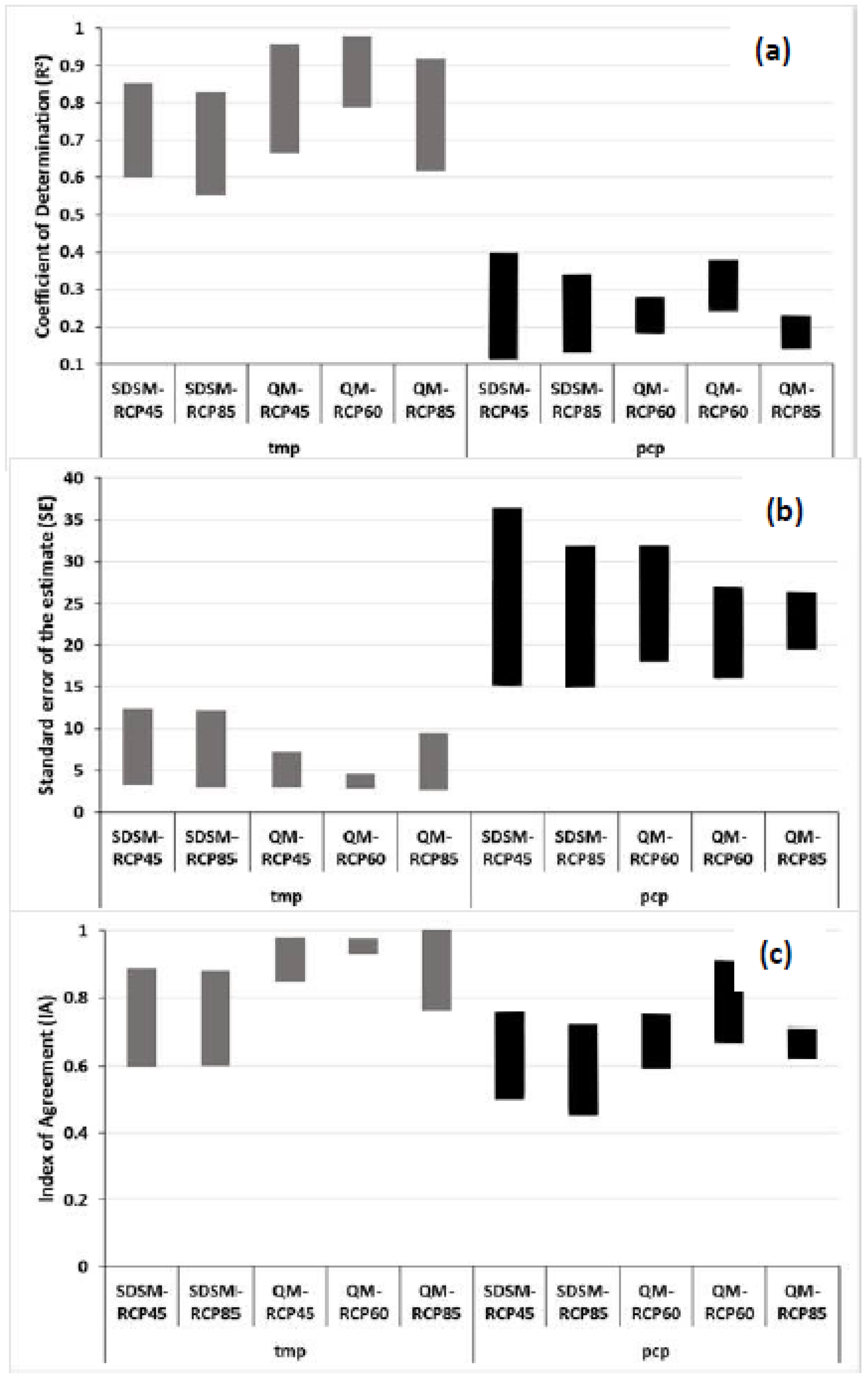
4.2. QM-Downscaling of Temperatures and Precipitation
4.2.1. Selecting the GCM Model for QM
4.2.2. Calibration and Validation of the QM Model
4.3. 2006–2015 Projections of Temperatures and Precipitation
4.4. Future Projections of Temperature and Precipitation
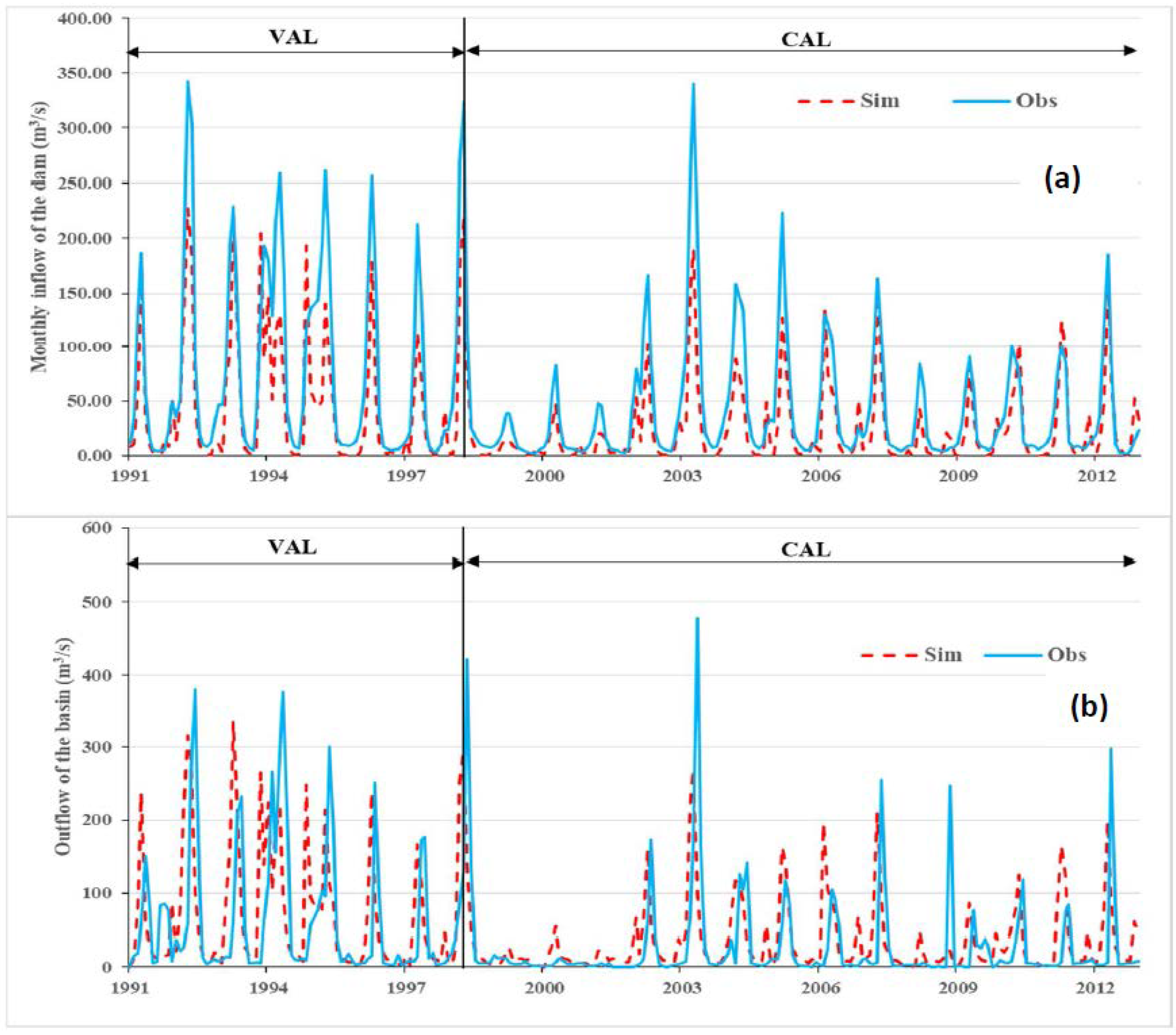
4.5. Calibration and Validation of the SWAT Model
4.6. Climate Change Impacts on the Zarrine River Basin (ZRB) Hydrology and Water Resources
4.6.1. SWAT-Simulated Future Stream Inflow to the Boukan Dam
4.6.2. SWAT-Predicted Future Water Balance Parameters for the ZRB
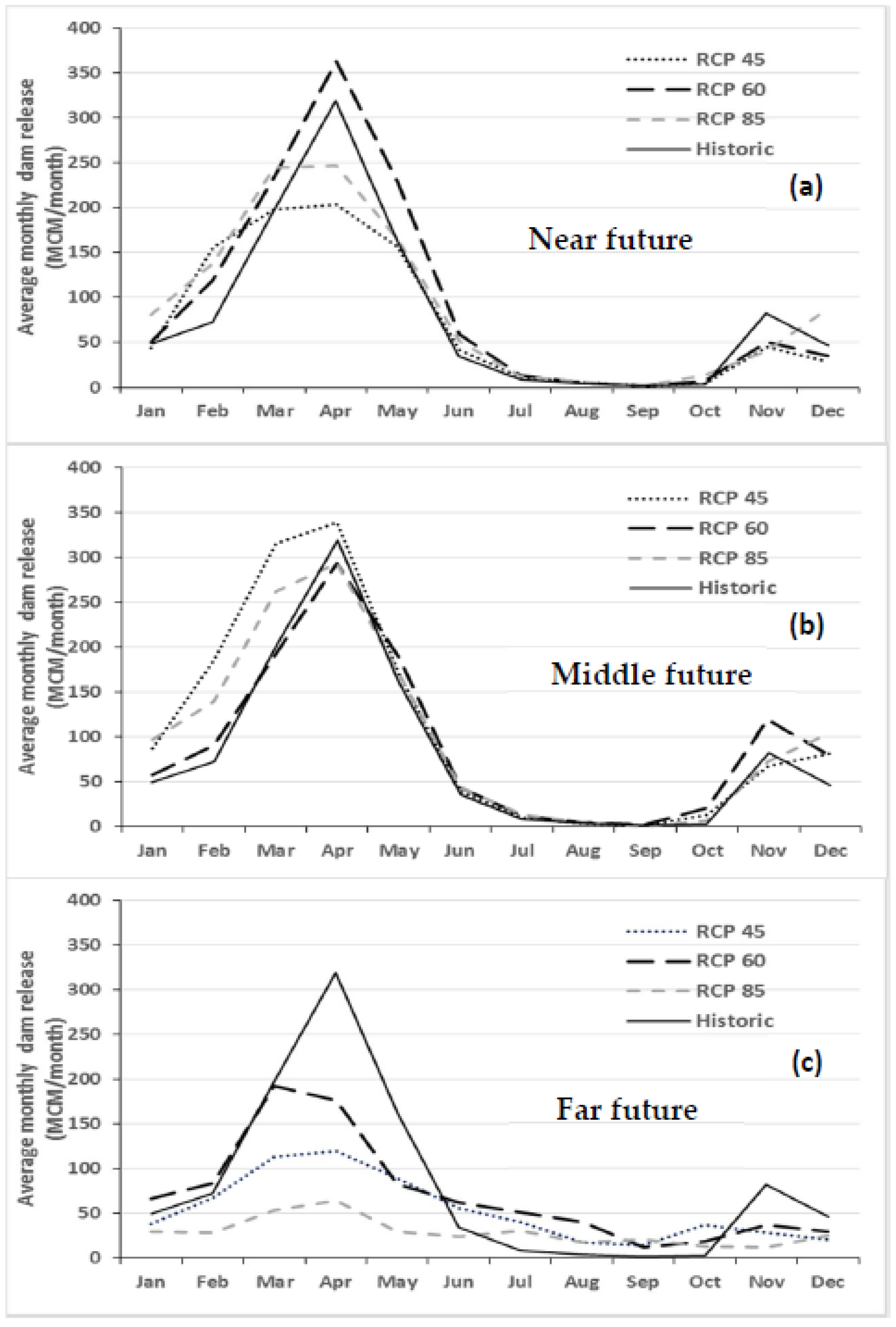
4.6.3. Future Dependable Reservoir Water Release (DWR)
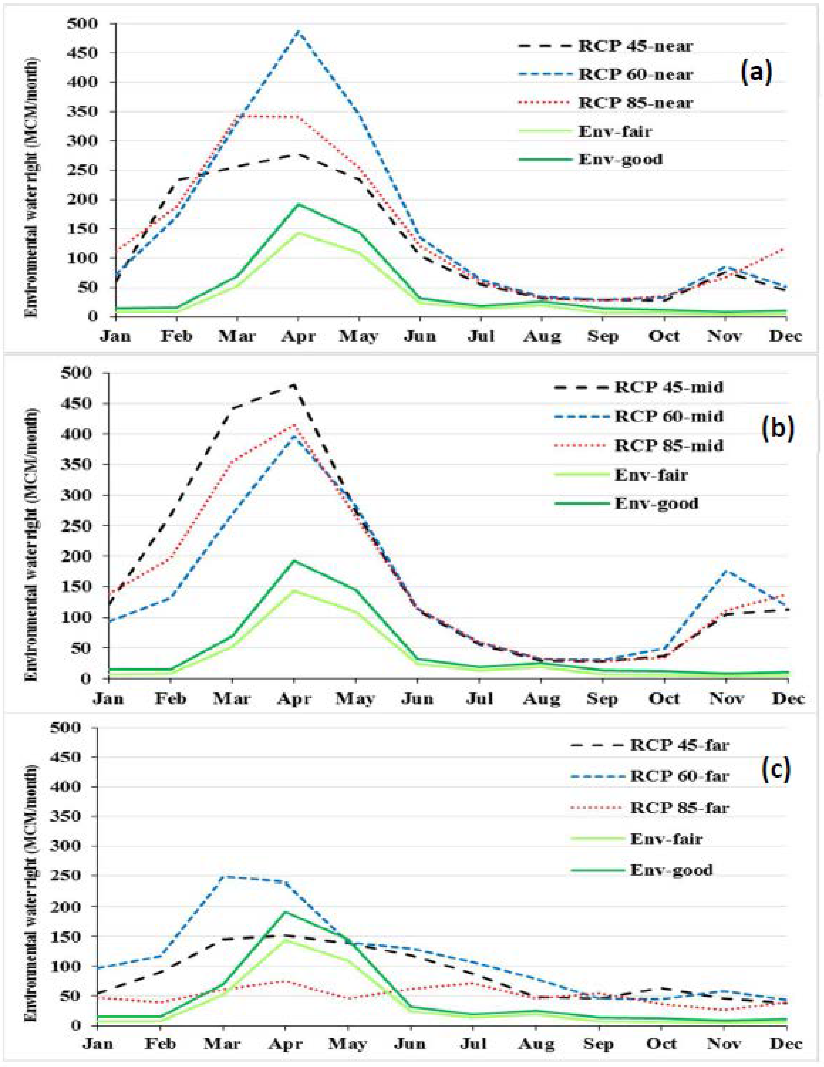
4.6.4. Future Monthly Environmental Water Demands of the ZR
5. Summary and Conclusions
Author Contributions
Conflicts of Interest
References
- Hijioka, Y.; Lin, E.; Pereira, J.J.; Corlett, R.T.; Cui, X.; Insarov, G.E.; Lasco, R.D.; Lindgren, E.; Surjan, A. Asia. In Climate Change 2014: Impacts, Adaptation, and Vulnerability. Part B: Regional Aspects; Contribution of Working Group II to the Fifth Assessment Report of the Intergovernmental Panel on Climate Change; Cambridge University Press: Cambridge, UK, 2014; pp. 1327–1370. [Google Scholar]
- Intergovernmental Panel on Climate Change (IPCC). Climate Change 2007: The Physical Science Basis; Contribution of Working Group I to the Fourth Assessment Report of the Intergovernmental Panel on Climate Change; Cambridge University Press: Cambridge, UK, 2007. [Google Scholar]
- Intergovernmental Panel on Climate Change (IPCC). Climate Change 2014—Impacts, Adaptation and Vulnerability: Regional Aspects; Cambridge University Press: Cambridge, UK, 2014. [Google Scholar]
- Hagemann, S.; Chen, C.; Clark, D.; Folwell, S.; Gosling, S.N.; Haddeland, I.; Hannasaki, N.; Heinke, J.; Ludwig, F.; Voss, F.; et al. Climate change impact on available water resources obtained using multiple global climate and hydrology models. Earth Syst. Dyn. 2013, 4, 129–144. [Google Scholar] [CrossRef]
- Christensen, N.S.; Wood, A.W.; Voisin, N.; Lettenmaier, D.P.; Palmer, R.N. The effects of climate change on the hydrology and water resources of the Colorado River basin. Clim. Chang. 2004, 62, 337–363. [Google Scholar] [CrossRef]
- Terink, W.; Immerzeel, W.W.; Droogers, P. Climate change projections of precipitation and reference evapotranspiration for the Middle East and Northern Africa until 2050. Int. J. Clim. 2013, 33, 3055–3072. [Google Scholar] [CrossRef]
- World Health Organization (WHO). Climate and Health Country Profile 2015: Iran. WHO, 2015. Available online: http://www.who.int/iris/handle/10665/246125 (accessed on 22 December 2017).
- Teutschbein, C.; Wetterhall, F.; Seibert, J. Evaluation of different downscaling techniques for hydrological climate-change impact studies at the catchment scale. Clim. Dyn. 2011, 37, 2087–2105. [Google Scholar] [CrossRef]
- Reder, A.; Rianna, G.; Vezzoli, R.; Mercogliano, P. Assessment of possible impacts of climate change on the hydrological regimes of different regions in China. Adv. Clim. Chang. Res. 2016, 7, 169–184. [Google Scholar] [CrossRef]
- Emami, F.; Koch, M. Modeling the Impact of Climate Change on Water Availability in the Zarrine River Basin and Inflow to the Boukan Dam, Iran. Ecohydrol. Hydrobiol. 2017, in press. [Google Scholar]
- Sachindra, D.A.; Huang, F.; Barton, A.; Perera, B.J.C. Statistical downscaling of general circulation model outputs to precipitation—Part 1: Calibration and validation. Int. J. Climatol. 2014, 34, 3264–3281. [Google Scholar] [CrossRef]
- Wilby, R.L.; Dawson, C.W. The Statistical DownScaling Model (SDSM): Insights from one decade of application. Int. J. Climatol. 2013, 33, 1707–1719. [Google Scholar] [CrossRef]
- Emami, F.; Koch, M. Evaluating the water resources and operation of the Boukan Dam in Iran under climate change. Eur. Water 2017, 59, 17–24. [Google Scholar]
- Emami, F. Development of an Algorithm for Assessing the Impacts of Climate Change on Operation of Reservoirs. Master’s Dissertation, University of Tehran, Tehran, Iran, 2009. [Google Scholar]
- Wilby, R.L.; Dawson, C.W.; Barrow, E.M. SDSM—A decision support tool for the assessment of regional climate change impacts. Environ. Model. Softw. 2002, 17, 145–157. [Google Scholar] [CrossRef]
- AghaKouchak, A.; Norouzi, H.; Madani, K.; Mirchi, A.; Azarderakhsh, M.; Nazemi, A.; Nasrollahi, N.; Farahmand, A.; Mehran, A.; Hasanzadeh, E. Aral Sea syndrome desiccates Lake Urmia: Call for action. J. Great Lakes Res. 2015, 41, 307–311. [Google Scholar] [CrossRef]
- McSweeney, C.F.; Jones, R.G.; Lee, R.W.; Rowell, D.P. Selecting CMIP5 GCMs for downscaling over multiple regions. Clim. Dyn. 2015, 44, 3237–3260. [Google Scholar] [CrossRef]
- Lutz, A.F.; ter Maat, H.W.; Biemans, H.; Shrestha, A.B.; Wester, P.; Immerzeel, W.W. Selecting representative climate models for climate change impact studies: An advanced envelope-based selection approach. Int. J. Climatol. 2016, 36, 3988–4005. [Google Scholar] [CrossRef]
- Fu, G.; Liu, Z.; Charles, S.P.; Xu, Z.; Yao, Z. A score-based method for assessing the performance of GCMs: A case study of southeastern Australia. J. Geophys. Res. Atmos. 2013, 118, 4154–4167. [Google Scholar] [CrossRef]
- Mehran, A.; AghaKouchak, A.; Phillips, T.J. Evaluation of CMIP5 continental precipitation simulations relative to satellite-based gauge-adjusted observations. J. Geophys. Res. Atmos. 2014, 119, 1695–1707. [Google Scholar] [CrossRef]
- Van Vliet, J.; den Elzen, M.G.; van Vuuren, D.P. Meeting radiative forcing targets under delayed participation. Energy Econ. 2009, 31, 152–162. [Google Scholar] [CrossRef]
- Mora, C.; Frazier, A.G.; Longman, R.J.; Dacks, R.S.; Walton, M.M.; Tong, E.J.; Sanchez, J.J.; Kaiser, L.R.; Stender, Y.O.; Anderson, J.M.; et al. The projected timing of climate departure from recent variability. Nature 2013, 502, 183–187. [Google Scholar] [CrossRef] [PubMed]
- Peters, G.P.; Andrew, R.M.; Boden, T.; Canadell, J.G.; Ciais, P.; Le Quéré, C.; Wilson, C. The challenge to keep global warming below 2 C. Nat. Clim. Chang. 2013, 3, 4–6. [Google Scholar] [CrossRef]
- Wilby, R.L.; Dawson, C.W. SDSM 4.2—A Decision Support Tool for the Assessment of Regional Climate Change Impacts; User Manual; Lancaster University: Lancaster, UK, 2007. [Google Scholar]
- Hempel, S.; Frieler, K.; Warszawski, L.; Schewe, J.; Piontek, F. A trend-preserving bias correction-the ISI-MIP approach. Earth Syst. Dyn. 2013, 4, 219–236. [Google Scholar] [CrossRef]
- Miao, C.; Su, L.; Sun, Q.; Duan, Q. A nonstationary bias-correction technique to remove bias in GCM simulations. J. Geophys. Res. Atmos. 2016, 121, 5718–5735. [Google Scholar] [CrossRef]
- Themeßl, J.M.; Gobiet, A.; Leuprecht, A. Empirical-statistical downscaling and error correction of daily precipitation from regional climate models. Int. J. Climatol. 2011, 31, 1530–1544. [Google Scholar] [CrossRef]
- Li, H.; Sheffield, J.; Wood, E.F. Bias correction of monthly precipitation and temperature fields from Intergovernmental Panel on Climate Change AR4 models using equidistant quantile matching. J. Geophys. Res. 2010, 115. [Google Scholar] [CrossRef]
- Wang, L.; Chen, W. A CMIP5 multimodel projection of future temperature, precipitation, and climatological drought in China. Int. J. Climatol. 2014, 34, 2059–2078. [Google Scholar] [CrossRef]
- Gassman, P.W.; Reyes, M.R.; Green, C.H.; Arnold, J.G. The Soil and Water Assessment Tool: Historical Development, Applications, and Future Research Directions. Trans. ASABE 2007, 50, 1211–1250. [Google Scholar] [CrossRef]
- Neitsch, S.L.; Arnold, J.G.; Kiniry, J.R.; Williams, J.R. Soil and Water Assessment Tool Theoretical Documentation Version 2009; Texas Water Resources Institute: Temple, TX, USA, 2011. [Google Scholar]
- Devkota, L.P.; Gyawali, D.R. Impacts of climate change on hydrological regime and water resources management of the Koshi River Basin, Nepal. J. Hydrol. Reg. Stud. 2015, 4, 502–515. [Google Scholar] [CrossRef]
- Perazzoli, M.; Pinheiro, A.; Kaufmann, V. Assessing the impact of climate change scenarios on water resources in southern Brazil. Hydrol. Sci. J. 2013, 58, 77–87. [Google Scholar] [CrossRef]
- Tan, M.L.; Yusop, Z.; Chua, V.P.; Chan, N.W. Climate change impacts under CMIP5 RCP scenarios on water resources of the Kelantan River Basin, Malaysia. Atmos. Res. 2017, 189, 1–10. [Google Scholar] [CrossRef]
- Abbaspour, K.C.; Faramarzi, M.; Ghasemi, S.S.; Yang, H. Assessing the impact of climate change on water resources in Iran. Water Resour. Res. 2009, 45. [Google Scholar] [CrossRef]
- Ministry of the Energy (MOE). Updating of Water Master Plan of Iran; Water and Wastewater Macro Planning Bureau: Tehran, Iran, 2014.
- Fereidoon, M.; Koch, M. SWAT-Model based Identification of Watershed Components in a semi-arid Region with long term Gaps in the climatological Parameters’ Database. In Proceedings of the SGEM Vienna Green 2016, Vienna, Austria, 2–5 November 2016; The International Multidisciplinary Scientific GeoConferences SGEM: Vienna, Austria, 2016. Book 3. Volume 3, pp. 281–288. [Google Scholar]
- Arnold, J.G.; Moriasi, D.N.; Gassman, P.W.; Abbaspour, K.C.; White, M.J.; Srinivasan, R.; Santhi, C.; Harmel, R.D.; van Griensven, A.; van Liew, M.W.; et al. SWAT: Model Use, Calibration, and Validation. Trans. ASABE 2012, 55, 1491–1508. [Google Scholar] [CrossRef]
- Zhang, X.; Srinivasan, R.; Zhao, K.; Liew, M.V. Evaluation of global optimization algorithms for parameter calibration of a computationally intensive hydrologic model. Hydrol. Process. 2009, 23, 430–441. [Google Scholar] [CrossRef]
- Abbaspour, K.C.; Johnson, C.A.; Van Genuchten, M.T. Estimating uncertain flow and transport parameters using a sequential uncertainty fitting procedure. Vadose Zone J. 2004, 3, 1340–1352. [Google Scholar] [CrossRef]
- Krause, P.; Boyle, D.P.; Bäse, F. Comparison of different efficiency criteria for hydrological model assessment. Adv. Geosci. 2005, 5, 89–97. [Google Scholar] [CrossRef]
- Ministry of the Energy (MOE). Executive Strategies for Decreasing 40% of Agricultural Water Demands in Zarrine and Simineh River Basins (Saeenghaleh and Miandoab Areas), Volume 7: Studies of Water Resources and Demands Planning and Management; Urmia Lake Restoration Committee, Ministry of the Energy: Tehran, Iran, 2016.
- Tennant, D.L. Instream Flow Regimens for Fish, Wildlife, Recreation and Related Environmental Resources. Fisheries 1976, 1, 6–10. [Google Scholar] [CrossRef]
- Willmott, C.J. On the validation of models. Phys. Geogr. 1981, 2, 184–194. [Google Scholar]
- Nazarenko, L.; Schmidt, G.A.; Miller, R.L.; Tausnev, N.; Kelley, M.; Ruedy, R.; Russell, G.L.; Aleinov, I.; Bauer, M.; Bauer, S.; et al. Future climate change under RCP emission scenarios with GISS ModelE2. J. Adv. Model. Earth Syst. 2015, 7, 244–267. [Google Scholar] [CrossRef]
- Held, I.M.; Soden, B.J. Robust responses of the hydrological cycle to global warming. J. Clim. 2006, 19, 5686–5699. [Google Scholar] [CrossRef]


| GCM Model | Atmospheric Grid | RCP45 | RCP60 | RCP85 | Source | |
|---|---|---|---|---|---|---|
| Latitude | Longitude | |||||
| CESM-CAM5 | 0.942 | 1.25 | ✓ | ✓ | ✓ | National Science Foundation, Department of Energy, National Center for Atmospheric Research, USA |
| CCSM4 | 0.942 | 1.25 | ✓ | ✓ | ✓ | National Center for Atmospheric Research, USA |
| MRI-CGCM3 | 1.121 | 1.125 | ✓ | ✓ | ✓ | Meteorological Research Institute, Japan |
| MIROC5 | 1.401 | 1.406 | ✓ | ✓ | ✓ | Atmosphere and Ocean Research Institute, University of Tokyo, Japan |
| CNRM-CM5 | 1.401 | 1.406 | ✓ | ✘ | ✓ | Centre National de Recherches Meteorologiques, France |
| CMCC-CM | 0.75 | 0.75 | ✓ | ✘ | ✓ | Centro Euro-Mediterraneo per I Cambiamenti Climatici, Italy |
| Station | Tmp Max. | Tmp Min. | Effective Predictors | ||||||
|---|---|---|---|---|---|---|---|---|---|
| CAL | VAL | CAL | VAL | ||||||
| R2 | SE | R2 | SE | R2 | SE | R2 | SE | ||
| St1 | 0.77 | 2.1 | 0.94 | 2.8 | 0.63 | 2.1 | 0.90 | 2.6 | 500 hPa Geopotential 850 hPa Specific humidity 1000 hPa Specific humidity Air temperature at 2 m |
| St2 | 0.80 | 1.7 | 0.96 | 2.4 | 0.75 | 1.7 | 0.94 | 2.2 | 850 hPa Specific humidity 1000 hPa Specific humidity Air temperature at 2 m |
| St3 | 0.79 | 1.9 | 0.95 | 2.7 | 0.60 | 2.9 | 0.81 | 3.5 | 500 hPa Geopotential 1000 hPa Specific humidity Air temperature at 2 m |
| St4 | 0.81 | 1.7 | 0.96 | 2.3 | 0.63 | 2.4 | 0.87 | 2.9 | 500 hPa Geopotential 850 hPa Specific humidity 1000 hPa Specific humidity Air temperature at 2 m |
| St5 | 0.78 | 1.8 | 0.96 | 2.4 | 0.65 | 2.1 | 0.91 | 2.5 | 500 hPa Geopotential 850 hPa Specific humidity 1000 hPa Specific humidity Air temperature at 2 m |
| St6 | 0.82 | 1.7 | 0.95 | 2.8 | 0.71 | 1.7 | 0.90 | 2.6 | 500 hPa Geopotential 850 hPa Specific humidity 1000 hPa Specific humidity Air temperature at 2 m |
| Station | CAL | VAL | Effective Predictors | ||
|---|---|---|---|---|---|
| R2 | SE | R2 | SE | ||
| St1 | 0.33 | 4.8 | 0.35 | 3.2 | 500 hPa Meridional wind component 500 hPa Geopotential height 850 hPa Divergence of true wind 500 hPa Specific humidity Total precipitation |
| St2 | 0.28 | 4.7 | 0.26 | 2.6 | 500 hPa Meridional wind component 850 hPa Divergence of true wind 500 hPa Specific humidity Total precipitation |
| St3 | 0.3 | 6.3 | 0.30 | 3.6 | 500 hPa Meridional wind component 850 hPa Divergence of true wind Total precipitation |
| St4 | 0.26 | 2.7 | 0.20 | 2.0 | 1000 hPa Divergence of true wind 500 hPa Specific humidity 850 hPa Specific humidity Total precipitation |
| St5 | 0.25 | 5.3 | 0.28 | 3.1 | 1000 hPa Divergence of true wind 500 hPa Specific humidity 850 hPa Specific humidity Total precipitation |
| St6 | 0.49 | 2.7 | 0.15 | 2.8 | 500 hPa Specific humidity 850 hPa Specific humidity Total precipitation |
| Factor | Model | St1 | St2 | St3 | St4 | St5 | St6 | Skill Score | Final Score | |
|---|---|---|---|---|---|---|---|---|---|---|
| B | CESM-CAM5 | 0.83 | 1.02 | 1.72 | 2.30 | 1.97 | 1.03 | 2 | 2.5 | |
| CCSM4 | 0.88 | 0.91 | 1.70 | 2.17 | 1.93 | 0.94 | 4 | 3.0 | ||
| MRI-CGCM3 | 0.90 | 0.67 | 1.89 | 2.05 | 2.47 | 0.87 | 3 | 3.3 | ||
| MIROC5 | 1.53 | 1.14 | 3.05 | 2.80 | 3.38 | 1.16 | 1 | 1.2 | ||
| NRMSE | CESM-CAM5 | 0.68 | 0.61 | 1.74 | 2.05 | 2.09 | 0.66 | 2 | ||
| CCSM4 | 0.64 | 0.59 | 1.57 | 1.90 | 1.96 | 0.63 | 3 | |||
| MRI-CGCM3 | 0.30 | 0.43 | 1.21 | 1.27 | 1.68 | 0.27 | 4 | |||
| MIROC5 | 1.85 | 1.14 | 5.03 | 4.69 | 5.86 | 1.30 | 1 | |||
| R2 | CESM-CAM5 | 0.58 | 0.58 | 0.58 | 0.56 | 0.53 | 0.55 | 4 | ||
| CCSM4 | 0.61 | 0.61 | 0.61 | 0.59 | 0.58 | 0.58 | 3 | |||
| MRI-CGCM3 | 0.92 | 0.90 | 0.92 | 0.92 | 0.88 | 0.88 | 1 | |||
| MIROC5 | 0.64 | 0.64 | 0.66 | 0.64 | 0.59 | 0.61 | 2 | |||
| QBt | 25th | CESM-CAM5 | 0.92 | 1.04 | 1.39 | 1.63 | 1.38 | 1.07 | 2 | |
| 50th | 0.98 | 1.05 | 1.34 | 1.50 | 1.29 | 1.07 | 2 | |||
| 75th | 1.03 | 1.08 | 1.32 | 1.43 | 1.26 | 1.09 | 3 | |||
| 25th | CCSM4 | 0.96 | 0.93 | 1.37 | 1.50 | 1.40 | 0.96 | 3 | ||
| 50th | 1.02 | 0.80 | 1.34 | 1.43 | 1.33 | 1.00 | 3 | |||
| 75th | 1.09 | 1.03 | 1.35 | 1.40 | 1.33 | 1.05 | 2 | |||
| 25th | MRI-CGCM3 | 0.95 | 0.79 | 1.41 | 1.47 | 1.54 | 0.91 | 4 | ||
| 50th | 1.00 | 0.85 | 1.36 | 1.38 | 1.43 | 0.95 | 4 | |||
| 75th | 1.07 | 0.93 | 1.35 | 1.36 | 1.40 | 1.00 | 4 | |||
| 25th | MIROC5 | 1.39 | 1.09 | 1.99 | 1.80 | 1.90 | 1.10 | 1 | ||
| 50th | 1.34 | 1.07 | 1.76 | 1.62 | 1.66 | 1.08 | 1 | |||
| 75th | 1.34 | 1.07 | 1.64 | 1.52 | 1.57 | 1.08 | 1 | |||
| Factor | Model | St1 | St2 | St3 | St4 | St5 | St6 | Skill Score | Final Score | |
|---|---|---|---|---|---|---|---|---|---|---|
| B | CESM-CAM5 | 0.94 | 1.04 | 0.81 | 1.47 | 0.93 | 1.02 | 6 | 5.7 | |
| CCSM4 | 1.23 | 1.27 | 0.95 | 1.76 | 1.09 | 1.24 | 4 | 3.7 | ||
| MRI-CGCM3 | 1.51 | 2.11 | 1.23 | 2.45 | 1.42 | 1.61 | 2 | 2.7 | ||
| MIROC5 | 0.77 | 1.58 | 0.68 | 1.91 | 1.10 | 1.21 | 5 | 4.7 | ||
| CNRM-CM5 | 0.94 | 2.14 | 0.83 | 3.13 | 1.81 | 1.63 | 1 | 1.8 | ||
| CMCC-CC | 1.48 | 1.13 | 1.34 | 2.01 | 1.42 | 0.86 | 3 | 2.5 | ||
| NRMSE | CESM-CAM5 | 1.25 | 1.19 | 1.26 | 1.62 | 1.30 | 1.11 | 6 | ||
| CCSM4 | 1.43 | 1.31 | 1.32 | 1.87 | 1.40 | 1.31 | 4 | |||
| MRI-CGCM3 | 1.57 | 1.95 | 1.34 | 2.56 | 1.40 | 1.50 | 3 | |||
| MIROC5 | 1.05 | 1.55 | 1.15 | 1.90 | 1.20 | 1.27 | 5 | |||
| CNRM- CM5 | 1.11 | 2.14 | 1.13 | 3.35 | 1.70 | 1.62 | 1 | |||
| CMCC-CC | 1.65 | 1.52 | 1.77 | 2.42 | 1.83 | 1.40 | 2 | |||
| R2 | CESM-CAM5 | 0.08 | 0.08 | 0.08 | 0.05 | 0.06 | 0.17 | 4 | ||
| CCSM4 | 0.06 | 0.08 | 0.05 | 0.06 | 0.04 | 0.10 | 2 | |||
| MRI-CGCM3 | 0.12 | 0.16 | 0.08 | 0.10 | 0.11 | 0.12 | 5 | |||
| MIROC5 | 0.13 | 0.11 | 0.10 | 0.10 | 0.09 | 0.10 | 3 | |||
| CNRM | 0.18 | 0.09 | 0.18 | 0.13 | 0.18 | 0.09 | 6 | |||
| CMCC-CC | 0.16 | 0.00 | 0.00 | 0.00 | 0.00 | 0.00 | 1 | |||
| QBt | 25th | CESM-CAM5 | 0.94 | 1.00 | 0.80 | 1.46 | 0.92 | 1.00 | 6 | |
| 50th | 0.95 | 0.95 | 0.81 | 1.47 | 0.95 | 0.95 | 6 | |||
| 75th | 0.98 | 0.92 | 0.86 | 1.44 | 1.02 | 0.92 | 6 | |||
| 25th | CCSM4 | 1.23 | 1.24 | 0.95 | 1.76 | 1.09 | 1.23 | 4 | ||
| 50th | 1.21 | 1.16 | 0.94 | 1.73 | 1.10 | 1.16 | 4 | |||
| 75th | 1.22 | 1.10 | 0.94 | 1.67 | 1.11 | 1.09 | 4 | |||
| 25th | MRI-CGCM3 | 1.51 | 2.08 | 1.22 | 2.46 | 1.41 | 1.59 | 2 | ||
| 50th | 1.45 | 1.88 | 1.15 | 2.37 | 1.35 | 1.44 | 2 | |||
| 75th | 1.43 | 1.74 | 1.08 | 2.23 | 1.29 | 1.31 | 2 | |||
| 25th | MIROC5 | 0.77 | 1.55 | 0.68 | 1.90 | 1.09 | 1.18 | 5 | ||
| 50th | 0.75 | 1.48 | 0.65 | 1.84 | 1.05 | 1.12 | 5 | |||
| 75th | 0.73 | 1.40 | 0.63 | 1.74 | 1.01 | 1.06 | 5 | |||
| 25th | CNRM-CM5 | 0.93 | 2.07 | 0.82 | 3.10 | 1.78 | 1.58 | 1 | ||
| 50th | 0.95 | 1.95 | 0.83 | 3.04 | 1.73 | 1.48 | 1 | |||
| 75th | 0.97 | 1.83 | 0.84 | 2.87 | 1.66 | 1.38 | 1 | |||
| 25th | CMCC-CC | 1.49 | 1.13 | 1.34 | 2.03 | 1.43 | 0.87 | 3 | ||
| 50th | 1.56 | 1.11 | 1.35 | 2.05 | 1.47 | 0.84 | 3 | |||
| 75th | 1.56 | 1.06 | 1.28 | 1.94 | 1.42 | 0.80 | 3 | |||
| Model | Future Period | Scenario | ∆TMP (°C) | ∆PCP (%) |
|---|---|---|---|---|
| SDSM | Near | RCP45 | 1.39 | 8% |
| RCP85 | 1.58 | 15% | ||
| Mid | RCP45 | 2.58 | 12% | |
| RCP85 | 3.83 | 22% | ||
| Far | RCP45 | 3.25 | 13% | |
| RCP85 | 6.21 | 29% | ||
| QM | Near | RCP45 | 0.61 | −4% |
| RCP60 | 0.75 | 4% | ||
| RCP85 | 1.18 | 3% | ||
| Mid | RCP45 | 1.4 | 15% | |
| RCP60 | 1.51 | 3% | ||
| RCP85 | 2.85 | 17% | ||
| Far | RCP45 | 1.63 | −3% | |
| RCP60 | 2.2 | 13% | ||
| RCP85 | 4.7 | −19% |
| Rank | Parameter Name | Dimension | Final Value/Range | Rank | Parameter Name | Dimension | Final Value/Range |
|---|---|---|---|---|---|---|---|
| 1 | CN2.mgt | dimensionless | 59–90 | 13 | ALPHA_BNK.rte | days | 0.10–0.77 |
| 2 | GW_DELAY.gw | Day | 5–28 | 14 | SNOCOVMX.bsn 1 | mm | 116 |
| 3 | SOL_BD(1).sol | g/cm3 | 0.95–1.54 | 15 | SOL_Z(1).sol | mm | 281–392 |
| 4 | GW_REVAP.gw 1 | dimensionless | 0.037 | 16 | SNO50COV.bsn 1 | dimensionless | 0.57 |
| 5 | RCHRG_DP.gw 1 | dimensionless | 0.014 | 17 | SOL_K(1).sol | mm/h | 7.22–14 |
| 6 | REVAPMN.gw | mm H2O | 1–450 | 18 | TIMP.bsn 1 | dimensionless | 0.57 |
| 7 | ALPHA_BF.gw | 1/day | 0.03–0.75 | 19 | GWQMN.gw | mm H2O | 750–3514 |
| 8 | ESCO.hru | dimensionless | 0.51–0.99 | 20 | CH_N2.rte 1 | dimensionless | 0.016 |
| 9 | SFTMP.bsn 1 | °C | 1.93 | 21 | SMTMP.bsn 1 | °C | 1.08 |
| 10 | CH_K2.rte 1 | mm/h | 0.5 | 22 | GW_SPYLD.gw 1 | m3/m3 | 0.05 |
| 11 | SHALLST.gw | mm | 943–5000 | 23 | SMFMX.bsn 1 | mm H2O/°C-day | 7.95 |
| 12 | SOL_AWC(1).sol | mm H2O/mm | 0.14–0.24 | 24 | SMFMN.bsn 1 | mm H2O/°C-day | 0.73 |
| Streamflow Station | Calibration | Validation | ||||
|---|---|---|---|---|---|---|
| R2 | NS | bR2 | R2 | NS | bR2 | |
| Nezamabad | 0.7 | 0.69 | 0.47 | 0.65 | 0.62 | 0.48 |
| Chooblooche | 0.50 | 0.48 | 0.40 | 0.56 | 0.43 | 0.44 |
| Sarighamish | 0.65 | 0.65 | 0.50 | 0.60 | 0.55 | 0.47 |
| Boukan Dam | 0.85 | 0.72 | 0.51 | 0.77 | 0.65 | 0.48 |
| Safakhaneh | 0.57 | 0.55 | 0.45 | 0.59 | 0.49 | 0.40 |
| Sonateh | 0.72 | 0.67 | 0.56 | 0.77 | 0.75 | 0.70 |
| Average | 0.67 | 0.63 | 0.48 | 0.67 | 0.58 | 0.50 |
| Water Balance Parameter | Historical | Near Future | Middle Future | Far Future | Average | ||||||||
|---|---|---|---|---|---|---|---|---|---|---|---|---|---|
| RCP45 | RCP60 | RCP85 | RCP45 | RCP60 | RCP85 | RCP45 | RCP60 | RCP85 | RCP45 | RCP60 | RCP85 | ||
| PCP | 392 | −5% | 4% | 3% | 15% | 3% | 17% | −2% | 13% | −19% | 3% | 7% | 1% |
| SNM | 58 | 5% | 36% | −36% | −5% | −16% | −38% | −41% | −57% | −83% | −14% | −12% | −52% |
| ET | 290 | 5% | 3% | 6% | 10% | 7% | 19% | 25% | 36% | 14% | 13% | 16% | 13% |
| ∆SW 1 | 17 | −90 | −28 | −100 | −61 | −41 | −33 | −84 | −46 | −106 | −78 | −38 | −80 |
| SURQ | 46 | −13% | 13% | −24% | 11% | 2% | 2% | −37% | −24% | −63% | −13% | −2% | −28% |
| GWQ | 84 | −18% | 5% | −2% | 15% | −2% | 4% | −46% | −32% | −67% | −17% | −10% | −21% |
| LATQ | 38 | −16% | −8% | 21% | 21% | 3% | 24% | −11% | 13% | −26% | −3% | 3% | 5% |
| WYLD | 168 | −16% | 4% | −2% | 15% | 1% | 7% | −36% | −20% | −57% | −12% | −5% | −17% |
| Water Category | Historic | Near Future | Middle Future | Far Future | |||||||
|---|---|---|---|---|---|---|---|---|---|---|---|
| RCP45 | RCP60 | RCP85 | RCP45 | RCP60 | RCP85 | RCP45 | RCP60 | RCP85 | |||
| DWR (MCM/yr) | 983 | 896 | 1169 | 1092 | 1312 | 1106 | 1212 | 644 | 857 | 355 | |
| Demands (MCM/yr) | Current | 1030 | 1288 | 1373 | 1501 | ||||||
| Recommended | 943 | 1007 | 1136 | ||||||||
| Supplied Demand (%) | Current | 95% | 70% | 91% | 85% | 96% | 81% | 88% | 43% | 57% | 24% |
| Recommended | 95% | >100% | >100% | >100% | >100% | >100% | 57% | 75% | 31% | ||
| Water Category | Near Future | Middle Future | Far Future | |||||||||
|---|---|---|---|---|---|---|---|---|---|---|---|---|
| Demands (MCM/yr) | Pot | Env | Ind | Agr | Pot | Env | Ind | Agr | Pot | Env | Ind | Agr |
| Current | 229 | 383 | 20 | 656 | 300 | 383 | 34 | 656 | 442 | 383 | 20 | 656 |
| Recommended | 212 | 383 | 18 | 348 | 277 | 383 | 18 | 348 | 407 | 383 | 16 | 348 |
© 2018 by the authors. Licensee MDPI, Basel, Switzerland. This article is an open access article distributed under the terms and conditions of the Creative Commons Attribution (CC BY) license (http://creativecommons.org/licenses/by/4.0/).
Share and Cite
Emami, F.; Koch, M. Evaluation of Statistical-Downscaling/Bias-Correction Methods to Predict Hydrologic Responses to Climate Change in the Zarrine River Basin, Iran. Climate 2018, 6, 30. https://doi.org/10.3390/cli6020030
Emami F, Koch M. Evaluation of Statistical-Downscaling/Bias-Correction Methods to Predict Hydrologic Responses to Climate Change in the Zarrine River Basin, Iran. Climate. 2018; 6(2):30. https://doi.org/10.3390/cli6020030
Chicago/Turabian StyleEmami, Farzad, and Manfred Koch. 2018. "Evaluation of Statistical-Downscaling/Bias-Correction Methods to Predict Hydrologic Responses to Climate Change in the Zarrine River Basin, Iran" Climate 6, no. 2: 30. https://doi.org/10.3390/cli6020030
APA StyleEmami, F., & Koch, M. (2018). Evaluation of Statistical-Downscaling/Bias-Correction Methods to Predict Hydrologic Responses to Climate Change in the Zarrine River Basin, Iran. Climate, 6(2), 30. https://doi.org/10.3390/cli6020030