Article

Translating MC2 DGVM Results into Ecosystem Services for Climate Change Mitigation and Adaptation

by
Dominique Bachelet
1,*,
Kenneth Ferschweiler
2,
Timothy J. Sheehan
2,
Benjamin M. Sleeter
3 and
Zhiliang Zhu
4
1
Department of Biological and Ecological Engineering, Oregon State University, Corvallis, OR 97331, USA
2
Conservation Biology Institute, Corvallis, OR 97333, USA
3
U.S. Geological Survey, Western Geographic Science Center, Tacoma, WA 98402, USA
4
U.S. Geological Survey, National Center, Reston, VA 20192, USA
*
Author to whom correspondence should be addressed.
Climate 2018, 6(1), 1; https://doi.org/10.3390/cli6010001
Submission received: 1 December 2017 / Revised: 21 December 2017 / Accepted: 24 December 2017 / Published: 28 December 2017

Abstract

:
Ecosystem services (ES) were conceived to emphasize the role of ecological processes in supporting societal needs and to allow their inclusion in the decision-making process. Currently climate change mitigation is one of the most important services ecosystems can provide to enhance sinks of greenhouse gas emissions as the planet warms and related extreme events take their toll on societies. Because ES cannot always be directly measured and because measurements are often cost prohibitive, process-based models are used to estimate their supply, delivery and/or value. We ran the MC2 dynamic global vegetation model for the conterminous US with/without land use for several future scenarios. We translated results into key ES such as carbon sequestration, which contributes to climate regulation, into a regulatory service or aboveground forest carbon into timber biomass, a provisioning service, and evaluated constraints to maintain them. By comparing projections with/without land use we illustrated differences between managed and natural lands and provided information to help the valuation of societally relevant services.

1. Introduction

Ecosystem services (ES) were conceived to emphasize the role of ecological processes in supporting societal needs and to allow their inclusion in the decision-making process [1,2]. The valuation of these services however has been challenging when direct economic values are not apparent [3]. While not all services provided by ecosystems are marketable goods, their importance can be recognized as essential for future human wellbeing but hard to evaluate monetarily and thus often ignored in land management decisions. For example, timber supply is a well-documented commodity (provisioning service). But forests also provide significant climate mitigation potential (regulatory service): they capture atmospheric carbon from the atmosphere; they store this carbon in woody biomass and for even longer-term storage in the soil; they moderate land surface temperature variations through their canopy and understory structure [4,5]. This service however is more difficult to evaluate. Similarly, the valuation of the recreational and spiritual experience (cultural service) forests provide the general public should be used to better inform forest management strategies in the context of climate change.
Both forests and grasslands can have a central role not only in climate change mitigation but also in adaptation e.g., [6]. Mitigation intends to reduce greenhouse gas emissions or increase carbon capture while adaptation aspires to reduce the vulnerability of a system by either limiting its exposure, decreasing its sensitivity, or enhancing its adaptability to the changes at hand. While forests can mitigate some of the anthropogenic greenhouse gas emissions by capturing and storing large quantities of carbon, grasslands can also capture carbon by producing biomass in dry environments but also store most of it belowground, relatively safe from the potential wildfires that release much of the carbon stored aboveground [7,8]. Agroforestry, urban forestry, integrated fire management and grassland restoration are valuable mitigation and adaptation strategies for a world where the human footprint increasingly affects the health of populations.
Public agencies have been interested in ecosystem services because they can provide a consistent baseline for the valuation of multiple-use lands [9]. For example, the U.S. Forest Service has been including ecosystem services and particularly carbon capture and sequestration potential in all national forest management plans [10] and the Bureau of Land Management in collaboration with the U.S. Geological Survey (USGS) has been assessing the effectiveness of ecosystem service valuation for resource management decisions, also including carbon sequestration in rangeland soils [11].
Because ecosystem services (particularly regulating services) cannot always be directly measured and because measurements are often cost prohibitive, process-based models are used to estimate of ecosystem service supply, delivery and/or value [12]. We used results from a dynamic vegetation and fire model to provide indicators for three types of ES including a regulatory service (carbon sequestration potential), a provisioning service (timber production) and a supporting service (index of habitat stability) for the conterminous USA. Model results [13] were originally generated to complement results from a national carbon sequestration assessment, conducted by the U.S. Geological Survey (USGS) in response to requirements of the Energy Independence and Security Act (EISA; U.S. Congress, 2007). The objective of the National Ecosystem Carbon Sequestration Assessment was to evaluate policy-relevant carbon sequestration capacity in natural and managed ecosystems through management or restoration activities. We translated our model results into the alternative currency of ES to facilitate their interpretation by land managers.
To maintain consistency with the work of our collaborators from the LandCarbon project [14], we documented changes in ES only between historical conditions (1971–2000) and mid-century (2041–2070). We evaluated one provisioning (timber production) and one regulating service (carbon sequestration) that could be evaluated as a climate change mitigation option as well as factors that might reduce these services, such as loss of vigor (reduced forest production), carbon losses due to wildfires and climatic water deficit (causing drought stress and possibly mortality). We also looked at projected changes in vegetation cover, due to changes in both land use and climate, which affect habitat availability/suitability for wildlife, as well as at changes in long term soil carbon storage.

2. Materials and Methods

Limitations had been identified in the LandCarbon original methodology (the General Ensemble Biogeochemical Modeling System i.e., GEMS, [15]) that the MC2 model could address. First, changes in vegetation types as a result of climate change had not been simulated. Land use was imposed and natural vegetation was assumed to be stable while in MC2 a set of biogeography rules based on climatic thresholds allows vegetation shifts and post-fire pseudo-succession to occur. Ecological succession is the process of change in the species structure of an ecological community over time. Because MC2 does not simulate species we cannot use the term succession. However, after a fire that cause extensive tree mortality, the model will first grow the herbaceous cover and start growing small woody lifeforms competing with herbaceous lifeforms until conditions allow sufficient growth for woody lifeforms to start shading herbaceous lifeforms and competing effectively for available resources eventually closing the canopy and thus limiting herbaceous growth.
Secondly wildland fires had not been closely coupled with ecosystem processes and had simply consisted of another input to the model while in MC2 fuels loads are calculated based on plant growth and fire occurrence is simulated based on climate thresholds and (live and dead) fuels water content.
Furthermore, while instantaneous fire emissions had been calculated with GEMS, longer term fire effects on ecosystem productivity and carbon sequestration had not been analyzed. Third, the distinction between protected areas and managed lands was not simulated while MC2 could be run with and without land use, giving the ability to compare the role of human impact with that of climate alone.
Consequently, it is in the framework of the LandCarbon project that we used the dynamic global vegetation model (DGVM) MC2 e.g., [13,16] to simulate vegetation dynamics and associated carbon fluxes and stocks over the conterminous USA between 1895 and 2100 at 30 arcsec (~800 m) spatial resolution. MC2 includes a biogeography module that simulates potential vegetation types (Table A1). Each vegetation type is composed of a mixture of two lifeforms, herbaceous (including grasses, forbs) and woody (trees and shrubs), the relative dominance of which varies as a function of climatic conditions. Tree phenology (deciduousness or evergreenness) and leaf morphology (broadleaf or needleleaf) are determined at each annual time step as a function of the minimum temperature of the coldest month and of the growing (i.e., warm) season precipitation that have been smoothed over 15 years. The smoothing function progressively diminishes the influence of each past year’s climate on the smoothed climate variables to take into account the inherent inertia of long-lived woody types to short-term climate variability [17]. The C3/C4 grass functional types are determined by the ratio of C3/C4 grass productivity, which depends on the temperature of the three consecutive warmest months, subject to the same 15-year climate smoothing function. Warmer temperatures favor C4 grasses. The balance between woody and herbaceous lifeforms is determined by simulating the competition between the two for light, water and nutrients, as mediated by fire. The resulting biomasses along with smoothed climate thresholds are used to define the vegetation types.
MC2 includes a biogeochemistry module that tracks monthly carbon stocks in the soil as well as in diverse live and dead plant parts (leaves and roots, branches and boles). Plant growth is controlled by temperature, soil water, soil N, self-shading, and atmospheric CO2. Woody and herbaceous production rates are based on maximum monthly rates that are interpolated between lifeform-dependent parameter values, depending on the mixture of functional types set by the biogeography module. Mortality is driven by age and drought effect. A moderate CO2 fertilization effect increases production and water use efficiency such that when a concentration of 700 ppm atmospheric CO2 is reached, NPP has increased and transpiration has decreased linearly over time by 25%.
Decomposition rates are influenced by soil texture, soil moisture and temperature, as well as the existing soil carbon content and the nutrient content of the dead material. Based on the size and moisture content of the various types of fuel loads derived from carbon stocks, the model also simulates the occurrence and effects (plant mortality or consumption) of wildfires at a daily time step, modifying carbon stocks accordingly and allowing for a post-fire pseudo-succession, by simulating transitions between low biomass herbaceous-dominated ecosystem with regrowing woody plants and full canopy restored forests. Fluxes of water (potential and actual evapotranspiration, PET and AET) and carbon (net primary production—NPP, net biome production—NBP, heterotrophic respiration) are calculated annually and can therefore be used to estimate the supply of ES.
MC2 includes a fire module that includes a set of mechanistic fire behavior and effects functions [18,19,20] embedded in a structure that enables two-way interactions with the biogeochemistry and biogeography modules. Live and dead fuel loads in 1-h, 10-h, 100-h and 1000-h fuel classes are estimated from the carbon pools simulated in the biogeochemistry module. Allometric functions relate woody carbon pool sizes to height, crown base height and bark thickness for an average-sized tree. Empirical parameters are used to determine when crown (as opposed to surface) fires occur and project fire effects on vegetation (mortality only versus biomass consumption and emissions). The moisture content of the different fuel classes and the potential fire behavior are calculated each day based on pseudo-daily data interpolated from the monthly climate inputs. For temperature and relative humidity, a linear interpolation between monthly values is used to generate daily values. For precipitation, the number of precipitation events is estimated with a regression function derived from weather station data archived by the National Climate Data Center [21]. Monthly values are divided by the number of precipitation events per month and resulting values are randomly assigned to days within each month. Moisture contents of plant parts passed from the biogeochemistry module determine live fuel moisture contents. A combination of the Canadian Fine Fuel Moisture Code [22] and the National Fire Danger Rating System [23] is used to estimate dead fuel moisture contents. Potential fire behavior (including rate of spread) is calculated each day based on daily-interpolated fuel loads, moisture contents and weather. Potential fire behavior is modulated by vegetation type, which affects fuel properties and realized wind speeds (e.g., higher for grasslands than forests). Actual fire is simulated whenever the calculated rate of spread is greater than zero and user-specified thresholds are exceeded for the fine fuel moisture code (FFMC) and the build-up index (BUI) of the Canadian fire weather index system. These two indices are inverse functions of fine fuel and coarser fuel moisture contents, respectively, as specified by [22]. Only one fire is simulated per year per cell on the first day when all thresholds are exceeded. Note that the day and year of fire may vary from cell to cell, given the independent simulation of each cell.
Model inputs include soil characteristics (mineral depth, texture, bulk density) [24,25], atmospheric CO2 concentration (provided by R. Stouffer, pers. comm.) and monthly climate (minimum and maximum temperature, precipitation and vapor pressure). MC2 is run in four distinct successive phases: a first phase to initialize vegetation cover and carbon pools, a spinup phase to allow pools and vegetation dynamics to adjust in response to dynamic fire simulations, and a transient phase where historical and future climate time series are used to simulate past and future dynamics.
Historical climate data (1895–2010) were acquired from the PRISM group at Oregon State University [26] at 30 arcsec spatial resolution. To maintain consistency with LandCarbon methods [14], we used climate projections from CSIRO Mk3 [27], CGCM3 [28] and MIROC 3.2 medres [29] (henceforth CSIRO, CGCM3 and MIROC) for three emission scenarios A2, A1B and B1. Climate data were originally acquired from the WCRP (World Climate Research Programme) CMIP3 (Coupled Model Intercomparison Project phase 3) multi-model database website (https://esg.llnl.gov:8443/home/publicHomePage.do). They were then downscaled using the delta or anomaly method of [30]. Method details are available in (Appendix S1 in [13]).
The MC2 model was first used to simulate potential vegetation (PV) driven by climate and maintained by wildfires, without consideration of any human intervention. Küchler’s potential vegetation map of the United States [31] as well as [32]’s estimates of potential fire return interval (FRI) have been used as benchmarks for testing MC2 [13]. We also compared aboveground biomass results for the period 2000–2005 with estimates from the National Biomass and Carbon Dataset (NBCD) [33,34].
For another set of runs, land cover was simulated using contemporary and projected land use (LU) for each greenhouse gas emission scenario [35], with a legacy of fire suppression starting in 1950. We used future climate, CO2 concentrations and land use projections that were aligned with three Intergovernmental Panel on Climate Change (IPCC)’s greenhouse gas emission scenarios (A1B, A2 and B1) from the fourth assessment report [36]. To simulate the suppression of wildfires as a land-management practice, we used thresholds of fire line intensity, energy release component and rate of spread below which the fire routine was skipped assuming completely effective suppression [37]. We calibrated our initial results with land use to a variety of published estimates of carbon pools and fluxes (Figure S1 in [13]), as well as forest area and fire emissions [38].
Categorical variables such as potential vegetation and land use were summarized as modes for the historical period (1971–2000) and for the mid-century period (2041–2070) across the three climate model projections under the A2 future scenario. We aggregated model results into four broad categories and assigned numerical values to each: grasslands (1), shrublands (2), woodlands and forests (3), and other types (including deserts and barrens, as well as imposed agriculture/grazing, developed and mining, 0). This aggregation was based on carbon levels (units are g∙m−2) such that:
  • If herbaceous carbon stocks >200 g∙m−2 and woody carbon stocks <80 g∙m−2 we called it a grassland.
  • Then if woody carbon stocks >1150 g∙m−2 we called it a forest.
  • Then if woody carbon stocks >1 g∙m−2 we called it a shrubland.
  • The rest was called “other.”
We subtracted historical values for aggregated vegetation types from future values to calculate an index of habitat change ranging from −3 to +3. Differences between present and future conditions were rated as small to large depending on the type of transition that occurred. For example, a change from grassland (1) to forest (3) or the reverse (e.g., as a result of fire) would be large while a change from a conifer forest (3) to a mixed forest (3) would be small because the ecosystem function would not change dramatically.
Note that we used conventions from the ecological literature [39] where positive fluxes represent net carbon uptake by vegetation and soil, i.e., a carbon sink (removing carbon from the atmosphere), while negative fluxes represents a net release of carbon from the land to the atmosphere, i.e., a carbon source. Carbon sequestration (transfer from the atmosphere to any other carbon pool [39]) was calculated as the average net ecosystem production (NEP) i.e., net primary production minus soil heterotrophic respiration. Timber supply was estimated from the coarse wood pool. We applied the same method as [12] and assumed (1) that 60% of aboveground wood carbon could be used for timber production; (2) that biomass was composed of 45% carbon; and (3) that to obtain wood volume we could use the same conversion factor of 4 e−6∙m3/g C. Tree vigor, sensu [40], was calculated as the ratio of NPP over leaf area index (LAI) in forest areas where timber harvest is occurring. Loss of carbon to wildfires is calculated in the model routinely for every fire event. Wildlife habitat quality is evaluated as a function of the stability of the type of vegetation cover over time.
To make model results readily available to stakeholders in the state of California, we provide model results within the state borders on a web application (http://climateconsole.org) under the “Climate Impacts” tab, providing maps of vegetation dynamics as well as charts describing carbon fluxes and stocks in the state. Another web application provides the same service for the conterminous USA (http://climateconsole.org/conus) where the raw data are also available for download.

3. Simulation Results

3.1. Forest Area and Productivity, Relevant to Timber Supply as a Provisioning ES

Under historical conditions (1971–2000), simulated forested areas (without land use or fire suppression) occupy 57% of the map of potential vegetation and by the middle of the 21st century (2041–2070) their extent has increased by 3–9% except under MIROC A2. With land use and fire suppression, forested areas occupy only 44% of the map under historical conditions because a large fraction of the eastern US and the Midwest has been transformed by agriculture and development but their extent increases by up to 19% (CSIRO B1) by mid-21st century. While warming generally drives shifts upward in elevation at the expense of alpine systems and shifts westward at the Great Plains—eastern forests ecotone, fire suppression with land use causes extensive woody encroachment of western shrublands and grasslands (Figure 1).
However, decreases in forest carbon density are simulated under all climate and emission scenarios except under CGCM3 (+5%) and CSIRO A1B (+14%) without land use. Furthermore, our calculation of vigor (ratio of production over leaf area index) shows a decline with land use. Note that where low vigor numbers are calculated for the historic period, the light color areas on the map match fairly well the insect and disease detection survey summary maps available from the USFS Forest Health Technology Enterprise Team (www.fs.fed.us/foresthealth/technology/adsm.shtml accessed 22 July 2016).
When we compare carbon stocks or timber supply in GAP 1 and 2 protected areas (USGS terminology: GAP Status Codes 1 and 2 meet the definition of protected by IUCN as “A clearly defined geographical space, recognized, dedicated and managed, through legal or other effective means, to achieve the long-term conservation of nature with associated ecosystem services and cultural values.” These include national parks, wilderness areas, strict nature reserves and national monuments) versus managed lands (agriculture, urban, industrial, mining), we see a greater potential for production than in the currently protected areas (Table 1). This is partially due to the fact that the richer soils that could support high production of natural vegetation have already been requisitioned to support agriculture.

3.2. Carbon Sequestration and Losses to Wildfires as a Regulating ES

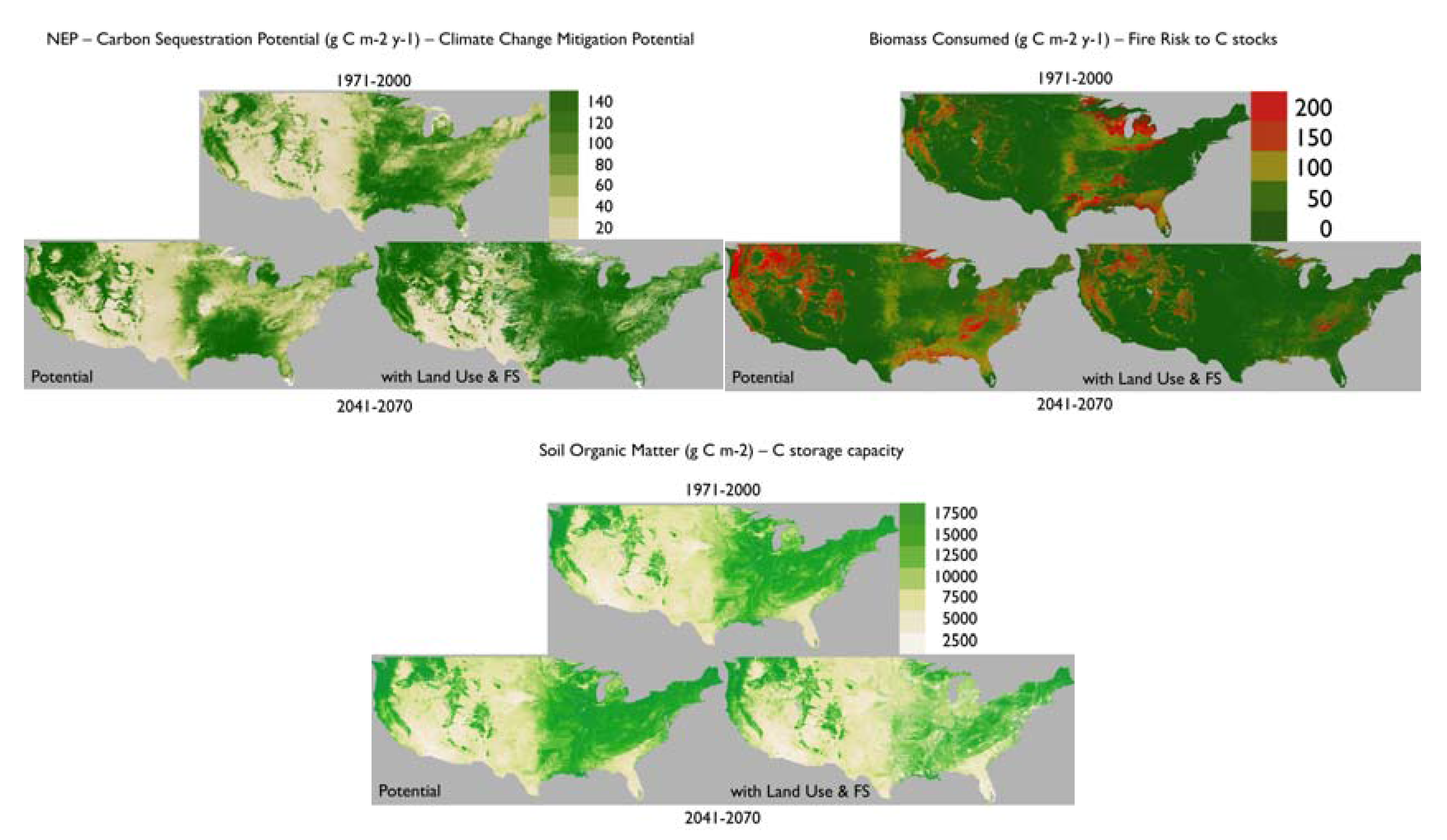
Net ecosystem production is the balance between net primary production and heterotrophic respiration. NEP increases under future climate scenarios (Figure 2) particularly with changes in land use. Without land use or fire suppression, senescence and mortality cause a significant respiration flux that reduces NEP. This process is missing in agriculture and urban areas but also in managed forest lands where harvest limits the size of the litter pool in the model. Moreover, in managed lands effective fire suppression could quadruple the carbon sequestration potential (Table 1) by allowing forest and woodland expansion at the expense of rangelands. On the other hand, litter production and accumulation without land use allow for the build-up of a soil carbon pool in natural areas, relatively safe from consumption by fire and thus ensuring its long-term storage. By mid-21st century, simulated soil carbon with land use and fire suppression had declined by up to 10% from historical levels to become 14 to 18% lower than in simulations results with wildfire and potential vegetation (Figure 2), regardless of the emission scenario or climate future we used. Carbon losses due to wildfires are limited by land use in managed areas (Table 1) due to the simple fact that agricultural and developed areas do not burn in the model and because fire suppression is assumed to be effective across the country. Note also that in our model results, fire suppression in protected areas does not affect carbon stocks or productivity remotely as much as in managed areas (Table 1), which is the kind of information that could inform future policies regarding fire management and resource allocation.

3.3. Vegetation Shifts That Will Affect Wildlife Habitat, a Supporting ES

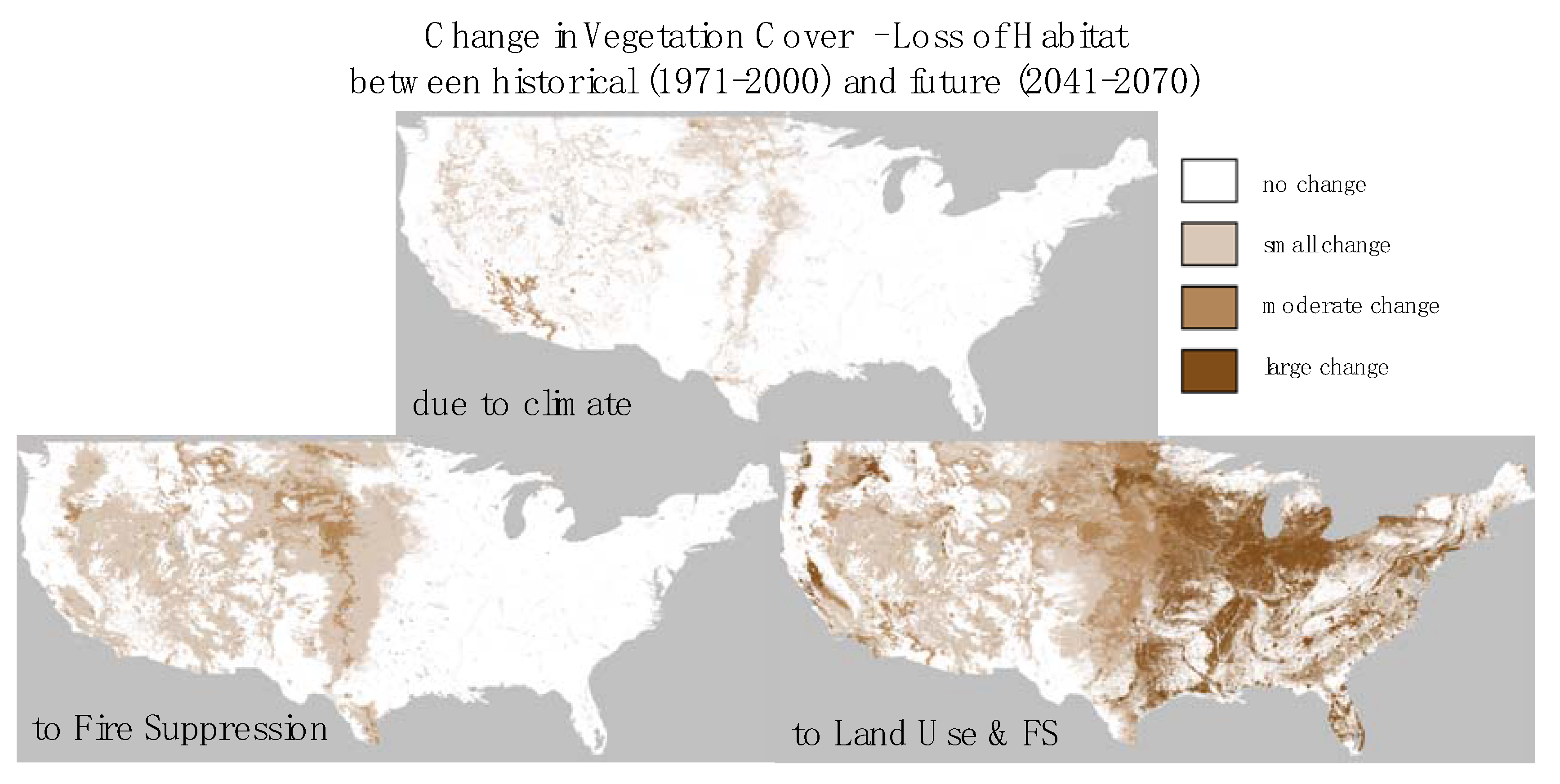
As [41] reminded us: “Ecosystem services have, by definition, an anthropocentric focus. They are the direct or indirect contributions from ecosystems to human welfare.” Biodiversity, which is often closely associated with ecosystem function, has been shown to directly enhance the provisioning of ecosystem services e.g., [42,43]. Habitat availability and quality are key ecosystem properties required to sustain a high level of biodiversity. To evaluate this aspect under climate change conditions, we have looked at the areas where vegetation shifts were simulated by our model (Figure 3) and assumed such changes would cause a level of stress to wildlife relying on stable habitats. Our assumption is of course an oversimplification since adaptation mechanisms have been reported in the literature whereby when vegetation cover changes, fauna dependent on it might migrate or switch associations e.g., [44]. Nevertheless, habitat loss due to land use and fire suppression (Figure 3) affects a much greater fraction of the conterminous than changes due only to climate change by mid-21st century reinforcing the general conclusion that human actions can affect species survival to a greater extent than climate which may however exacerbate the trend.

3.4. Limitations

Where the density of meteorological stations is low, the record length from existing meteorological stations is short, the infilling period important, or the topography complex, climate conditions and inter-annual variability within a grid cell may not be adequately represented by interpolation methods and climate models, imparting much uncertainty to the simulation of vegetation dynamics, related carbon and water fluxes and fire effects that depend on reliable climate inputs.
Similarly, the lack of reliable soil information e.g., [45], essential to simulate soil water availability, is affecting the robustness of our results. The coast-to-coast soils dataset used as input to MC2 is based on STATSGO [25,34] and has only been updated with SSURGO data in regions where those data were available [46]. Furthermore, where soil degradation has occurred due to past disturbances or a long legacy of land use has transformed land cover trajectories, simulations of land cover for the 20th century may not be based on accurate vegetation responses.
Apart from uncertainty in input values, simulating plant functional types may fail to take into account the role of human-introduced exotic invasives or leave out specific disturbance-resistant plant species, which can drive ecosystem processes in new directions and affect landscape resilience as well as adaptation capacity. Parameters used for a given plant functional group are often associated with the most “representative” species which, if inaccurate, could lead to an over or under-estimation of simulated ecosystem services.
The model was calibrated to best represent potential vegetation land cover from one coast to the other, matching [31]’s potential vegetation map of the United States. However, neither pest outbreaks nor extreme events such as wind throw, hurricanes, ice storms were included in the simulations. Past legacy of fire by native Americans were also not represented as a legacy constraint. Changes in land management practices such as fire suppression were simplified assuming no suppression before 1950 and effective suppression afterwards. Moreover, our land use assumptions were simple and would need to be revised before evaluating mitigation potential estimates.
Despite these limitations, very much in common with other DGVMs, the MC2 model fits in its role of “virtual laboratory” that can help “identify indicators of approaching, potentially irreversible, system thresholds or tipping points” [47].

4. Discussion

As Fisichelli [48] accurately observed, “climate change is a combination of directional shifts in baseline conditions (e.g., increasing mean temperatures) and changes in extreme events (e.g., more frequent and intense storms and droughts)” that will affect ecosystem processes and function in such a way as to modify the provision of ecosystem services our society has grown to depend on. Climate change combined with the legacy of land use (introduction of invasives, expansion of fire sensitive species due to 60+ years of suppression, expansion of agriculture and urban areas) will definitely challenge the adaptive capacity of ecosystems. The increase in atmospheric CO2 concentration however, by increasing both plant productivity and water use efficiency, may enhance the ability of vegetation cover to mitigate anthropogenic emissions. Our analysis hopes to increase the awareness of threats but also of opportunities which could help stimulate the development of adaptation options.
The increase in the total area of forests in the conterminous US (Figure 1) is driven, in the model, by both increased CO2 concentration that enhances WUE as well as some increase in precipitation allowing for woody encroachment in areas that were too dry for tree establishment a few decades ago. Furthermore, fire suppression and human land use have played a critical role in allowing widespread tree and shrub encroachment over the western US where grasslands and rangelands dominated the landscape. However, while our model does not simulate it, woody expansion has been accompanied with an expansion of invasive exotics that have modified the fire regime disallowing not only the expansion of the woody vegetation in some areas but also its survival in its current location, as fires became more frequent in arid zones [49]. Such complex and antagonistic biotic interactions are difficult to capture in models already limited by the uncertainty of their inputs (climate and soil). While these processes may have prevented a greater increase in carbon capture by woody vegetation, they have nonetheless increased the value of the carbon sequestration potential in grassland soils e.g., [50].
Despite its limitations, our model has shown that a warmer world will generally enhance carbon capture and timber production especially in areas where temperature is currently limiting growth and where future water availability is expected to be sufficient. Such optimism however needs to be dampened by the fact the model ignores possible damage by pests and pathogens that have already shown they could affect large swaths of forests [51,52,53]. To illustrate potential forest vulnerability to such outbreaks we mapped vigor (ratio of net primary production over leaf area index) in areas where forest productivity was simulated to be the highest (mean + .5* standard deviation) in the conterminous USA (Figure 4). We observed simulated future losses of vigor with land use, particularly worrisome where regional economies depend on the productivity of forest plantations, such as in the southeast where plantations and wood production for pellet production for international markets would be directly affected. So, in summary we have shown that the forests’ provisioning and regulating service may be reduced regionally by mid-century, a trend that might cause grave socioeconomic effects in areas where adaptive management strategies should already be envisaged [54]).
Further losses might be expected as forest production and thus fuels production increase in a warmer world: fuels will dry more easily with increased landscape fragmentation while longer fire seasons will increase the probability of human-caused ignitions and thus fire occurrence. Nonetheless, higher biomass production together with natural and disturbance-caused mortality are expected to increase soil carbon stocks, which are fairly resistant to losses from fires and thus should constitute effective long-term storage of carbon. With a more profound awareness of these negative as well as positive possible impacts of climate change on ecosystem processes, land managers should be able to better address the various challenges brought about by the combination of societal demands and climate-related threats.
Note that agriculture and urban areas are characterized in the model as exempt of fire. Globally, the decreasing trend in burned areas [55] is due to those same factors at work in the USA—agriculture expansion and urbanization. However, we have seen in California this Fall (2017) that urban areas, particularly the urban-wildland interface, can be vulnerable to fire, especially when policies allow for the expansion of development further away from urban centers into fire-prone landscapes. So, the fire risk to losses in carbon is real and includes a decrease in the reliability of long term storage categories such as construction timber.
Changes in vegetation cover (Figure 3) and fire regime due to climate and land use affect habitat quality for many organisms besides humans, positively for some, negatively for others. Fortunately, many species have already shown signs of adaptation [56,57,58,59]. While species distribution models have painted a dire future, they also have been shown to often overestimate extirpation by ignoring the complex biotic interactions and adaptive capacity of various species e.g., [60,61]. Nonetheless the supporting ES from existing ecosystems providing quality habitat for current species assemblages will be affected by climate change and natural resource managers need to start planning for “surprises” and novel ecosystems caused by complex interactions between climate and local environmental conditions e.g., [62]. Adaptive solutions such as assisted migration only confound the problem by stressing the recipient ecosystem that might have been stable until the transplanted organism was introduced. There have not been enough resources allocated to simply monitor the response of stressed species and gauge their specific adaptive capacity—generic diversity, dispersal capacity, phenotypic plasticity—to ensure that human intervention will be positive in the long term e.g., [63].

5. Conclusions

As a society, we have often assumed land management strategies will be sufficient to mitigate the negative effects of disturbance. However, history has shown that we were not always successful. For example, while Europeans have managed most of their forests, they have failed to optimize carbon sequestration because of timber exploitation and the establishment of dark evergreen plantations reducing reflectivity and enhancing surface warming [64]. Our society will need to further develop its capacity to adapt to change to not only mitigate the negative outcomes but also to be ready to take advantage of the opportunities climate change will bring to the land and enhance the natural adaptive capacity of existing ecosystems. It will be critical to estimate the value of areas (e.g., as in Table 1) that are best suited to be protected specifically to sequester carbon (a regulating service) compared to areas of timber production (a provisioning service) because trade-offs will be needed to balance the types of services society will need in the future [65]. If only provisioning services are valued, decision-makers could falsely believe that their choice of policies, new strategies and practices are improving our natural capital when critical ecological functions are in fact rapidly declining [12]. Practical interpretation of model results such as those from MC2 or others give managers some fodder to better evaluate the various futures that may develop before them and test options to manage or protect the land from further disturbance.
The striking differences between potential vegetation dynamics and land use-driven changes in land cover confirm the importance of the human footprint on ecosystem resilience to climate change and thus the availability of essential ecosystem services to mitigate human emissions in the future. The good news is that human activities can be changed and management strategies can be adapted to new conditions while plant and animal responses to climate change will vary based on the inherent adaptive capacity of individual species. This is a very positive conclusion because it means that we do have some control over much of the future of the land cover and could maintain its adaptive capacity by choosing appropriate management strategies.

Acknowledgments

Funding for this research was provided by the U.S. Geological Survey’s Climate and Land Use Program through USGS grant G12AC20214. The authors want to acknowledge Rama Nemani, NASA, for allowing them free access to the Pleiades NASA supercomputer.

Author Contributions

Dominique Bachelet conceived and designed the experiments. Kenneth Ferschweiler and Timothy Sheehan ran the model. Dominique Bachelet, Kenneth Ferschweiler and Timothy Sheehan analyzed the data. Benjamin M. Sleeter contributed land use data. Dominique Bachelet wrote the paper and made the revisions. Zhiliang Zhu contributed the LandCarbon methodology.

Conflicts of Interest

The authors declare no conflict of interest. The founding sponsor Zhiliang Zhu helped design the study to match the methodology used by the LandCarbon project collaborators.

Appendix A

Table A1. MC2 potential vegetation types.
1Undefined
2Ice or Barren (or Rock)
3Alpine or Arctic Tundra
4Taiga-Tundra
5Boreal Evergreen Needleleaf Forest
6Boreal Mixed Woodland
7Subalpine Forest
8Maritime Evergreen Needleleaf Forest
9Temperate Evergreen Needleleaf Forest
10Temperate Deciduous Broadleaf Forest
11Temperate Cool Mixed Forest
12Temperate Warm Mixed Forest
13Temperate Deciduous Broadleaf Woodland
14Temperate Cool Mixed Woodland
15Temperate Warm Mixed Woodland
16C3-Dominated and Temperate Shrubland
17C3-Dominated and Temperate Grassland
18Temperate Desert
19Subtropical Evergreen Needleleaf Forest
20Subtropical Deciduous Broadleaf Forest
21Subtropical Evergreen Broadleaf Forest
22Subtropical Mixed Forest
23Subtropical Evergreen Needleleaf Woodland
24Subtropical Deciduous Broadleaf Woodland
25Subtropical Evergreen Broadleaf Woodland
26Subtropical Mixed Woodland
27C4-Dominated Subtropical Shrubland
28C4-Dominated Subtropical Grassland
29Subtropical Desert
30Tropical Evergreen Broadleaf Forest
31Tropical Deciduous Woodland
32Tropical Savanna
33Tropical Shrubland
34Tropical Grassland
35Tropical Desert
36Cool Needleleaf Forest

References

  1. Daily, G.C.; Polasky, S.; Goldstein, J.; Kareiva, P.M.; Mooney, H.A.; Pejchar, L.; Ricketts, T.H.; Shallenberger, R. Ecosystem services in decision-making: Time to deliver. Front. Ecol. Environ. 2009, 7, 21–28. [Google Scholar] [CrossRef]
  2. Schmidt, K.; Sachse, R.; Walk, A. Current role of social benefits in ecosystem service assessments. Landsc. Urban Plan. 2016, 149, 49–64. [Google Scholar] [CrossRef]
  3. Scholes, R.J. Climate change and ecosystems. WIREs Clim. Chang. 2016. [Google Scholar] [CrossRef]
  4. Alkama, R.; Cescatti, A. Biophysical climate impacts of recent changes in global forest cover. Science 2016, 351, 600–604. [Google Scholar] [CrossRef] [PubMed] [Green Version]
  5. Frey, S.J.; Hadley, A.S.; Betts, M.G. Microclimate predicts within-season distribution dynamics of montane forest birds. Divers. Distrib. 2016, 22, 944–959. [Google Scholar] [CrossRef]
  6. Locatelli, B.; Pavageau, C.; Pramova, E.; di Gregorio, M. Integrating climate change mitigation and adaptation in agriculture and forestry: Opportunities and trade-offs. WIREs Clim. Chang. 2015, 6, 585–598. [Google Scholar] [CrossRef] [Green Version]
  7. Hu, S.; Chapin, F.S.; Firestone, M.K.; Field, C.B.; Chiariello, N.R. Nitrogen limitation of microbial decomposition in a grassland under elevated CO2. Nature 2001, 40, 188–191. [Google Scholar] [CrossRef] [PubMed]
  8. Ansley, R.J.; Boutton, T.W.; Skjemstad, J.O. Soil organic carbon and black carbon storage and dynamics under different fire regimes in temperate mixed-grass savanna. Glob. Biogeochem. Cycles 2006, 20, GB3006. [Google Scholar] [CrossRef]
  9. Ma, S.; Duggan, J.M.; Eichelberger, B.A.; McNally, B.W.; Foster, J.R.; Pepi, E.; Conte, M.N.; Daily, G.C.; Ziv, G. Valuation of ecosystem services to inform management of multiple-use landscapes. Ecosyst. Serv. 2016, 19, 6–18. [Google Scholar] [CrossRef]
  10. USDA (U.S. Department of Agriculture) Forest Service. National Forest System Land Management. Fed. Regist. 2012, 77, 21162–21276. [Google Scholar]
  11. Bagstad, K.J.; Semmens, D.; Winthrop, R.; Jaworski, D.; Larson, J. Ecosystem Services Valuation to Support Decision Making on Public Lands—A Case Study of the San Pedro River Watershed; Scientific Investigations Report 2012-5251; U.S. Geological Survey: Denver, CO, USA, 2012; p. 93.
  12. Karp, D.S.; Tallis, H.; Sachse, R.; Halpern, B.; Thonicke, K.; Cramer, W.; Mooney, H.; Polasky, S.; Tietjen, B.; Waha, K.; et al. National indicators for observing ecosystem service change. Glob. Environ. Chang. 2015, 35, 12–21. [Google Scholar] [CrossRef]
  13. Bachelet, D.; Ferschweiler, K.; Sheehan, T.; Sleeter, B.; Zhu, Z. Projected carbon stocks in the conterminous US with land use and variable fire regimes. Glob. Chang. Biol. 2015, 21, 4548–4560. [Google Scholar] [CrossRef] [PubMed]
  14. Zhu, Z.; Bergamaschi, B.; Bernknopf, R.; Clow, D.; Dye, D.; Faulkner, S.; Forney, W.; Gleason, R.; Hawbaker, T.; Liu, J. (Eds.) A Method for Assessing Carbon Stocks, Carbon Sequestration and Greenhouse-Gas Fluxes in Ecosystems of the United States under Present Conditions and Future Scenarios; Scientific Investigations Report 2010–5233; U.S. Geological Survey: Reston, VA, USA, 2010; p. 188.
  15. Liu, S.; Tan, Z.; Chen, M.; Liu, J.; Wein, A.; Li, Z.; Huang, S.; Oeding, J.; Young, C.; Verma, S.B.; et al. The General Ensemble Biochemical Modeling System (GEMS) and its applications to agricultural systems in the United States. In Managing Agricultural Greenhouse Gases—Coordinated Agricultural Research through GRACEnet to Address Our Changing Climate; Liebig, M.A., Franzluebbers, A.J., Follett, R.F., Eds.; Academic Press: London, UK, 2012; pp. 309–323. [Google Scholar]
  16. Sheehan, T.; Bachelet, D.; Ferschweiler, K. Projected major fire and vegetation changes in the Pacific Northwest of the conterminous United States under selected CMIP5 climate futures. Ecol. Model. 2015, 317, 16–29. [Google Scholar] [CrossRef]
  17. Daly, C.; Bachelet, D.; Lenihan, J.M.; Neilson, R.P. Dynamic simulation of tree-grass interactions for global change studies. Ecol. Appl. 2000, 10, 449–469. [Google Scholar]
  18. Rothermel, R.C. A Mathematical Model for Predicting Fire Spread in Wildland Fuels; USDA Forest Service Research Paper INT-115; Department of Agriculture, Intermountain Forest and Range Experiment Station: Ogden, UT, USA, 1972. [Google Scholar]
  19. Peterson, D.L.; Ryan, K.C. Modeling postfire conifer mortality for long-range planning. Environ. Manag. 1986, 10, 797–808. [Google Scholar] [CrossRef]
  20. Van Wagner, C. Prediction of crown fire behavior in two stands of jack pine. Can. J. For. Res. 1993, 23, 442–449. [Google Scholar] [CrossRef]
  21. Lenihan, J.M.; Daly, C.; Bachelet, D.; Neilson, R.P. Simulating broad-scale fire severity in a dynamic global vegetation model. Northwest Sci. 1998, 72, 91–101. [Google Scholar]
  22. Van Wagner, C.E.; Pickett, T.L. Equations and FORTRAN Program for the Canadian Forest Fire Weather Index System; Forestry Technical Report 33; Canadian Forestry Service, Petawawa National Forestry Institute: Chalk River, ON, Canada, 1985; p. 18. [Google Scholar]
  23. Bradshaw, L.S.; Deeming, J.E.; Burgan, R.E.; Cohen, J.D. The 1978 National Fire Danger Rating System: A Technical Documentation; General Technical Report INT-169; USDA Forest Service: Ogden, UT, USA, 1983.
  24. Kern, J.S. Spatial patterns of soil organic carbon in the contiguous United States. Soil Sci. Soc. Am. J. 1994, 58, 439–455. [Google Scholar] [CrossRef]
  25. Kern, J.S. Geographic patterns of soil water-holding capacity in the contiguous United States. Soil Sci. Soc. Am. J. 1995, 59, 1126–1133, Erratum in 2000, 64, 382. [Google Scholar] [CrossRef]
  26. Daly, C.; Halbleib, M.; Smith, J.I.; Gibson, W.P.; Doggett, M.K.; Taylor, G.H.; Curtis, J.; Pasteris, P.P. Physiographically sensitive mapping of climatological temperature and precipitation across the conterminous United States. Int. J. Climatol. 2008, 28, 2031–2064. [Google Scholar] [CrossRef]
  27. Gordon, H.B.; Rotstayn, L.D.; McGregor, J.L.; Dix, M.R.; Kowalczyk, E.A.; O’Farrell, S.P.; Waterman, L.J.; Hirst, A.C.; Wilson, S.G.; Collier, M.A.; et al. The CSIRO Mk3 Climate System Model; Technical Paper No. 60; CSIRO Atmospheric Research: Victoria, Australia, 2002. [Google Scholar]
  28. Boer, G.J. A hybrid moisture variable suitable for spectral GCMs. In Research Activities in Atmospheric and Oceanic Modelling; Report No. 21, WMO/TD-No. 665; World Meteorological Organization: Geneva, Switzerland, 1995. [Google Scholar]
  29. Hasumi, H.; Emori, S. (Eds.) K-1 Coupled GCM (MIROC) Description; K-1 Tech. Rep. 1; Center for Climate System Research: Tokyo, Japan, 2004. [Google Scholar]
  30. Fowler, H.J.; Blenkinsop, S.; Tebaldi, C. Linking climate change modelling to impacts studies: Recent advances in downscaling techniques for hydrological modeling. Int. J. Climatol. 2007, 27, 1547–1578. [Google Scholar] [CrossRef]
  31. Küchler, A. Potential Natural Vegetation of the United States, 2nd ed.; American Geographical Society: New York, NY, USA, 1975. [Google Scholar]
  32. Leenhouts, B. Assessment of biomass burning in the conterminous United States. Conserv. Ecol. 1998, 2, 1. [Google Scholar] [CrossRef]
  33. Kellndorfer, J.; Walker, W.; LaPoint, E.; Kirsch, K.; Bishop, J.; Fiske, G. Statistical fusion of lidar, InSAR, and optical remote sensing data for forest stand height characterization: A regional-scale method based on LVIS, SRTM, Landsat ETM+, and ancillary data sets. J. Geophys. Res. Biogeosci. 2010, 115. [Google Scholar] [CrossRef]
  34. Kellndorfer, J.; Walker, W.; Kirsch, K.; Fiske, G.; Bishop, J.; Lapoint, L.; Hoppus, M.; Westfall, J. NACP Aboveground Biomass and Carbon Baseline Data, V.2 (NBCD 2000), U.S.A., 2000; ORNL DAAC: Oak Ridge, TN, USA, 2013. Available online: https://daac.ornl.gov/cgi-bin/dsviewer.pl?ds_id=1161 (accessed on 26 December 2017).
  35. Sleeter, B.M.; Sohl, T.L.; Bouchard, M.A.; Reker, R.R.; Soulard, C.E.; Acevedo, W.; Griffith, G.E.; Sleeter, R.R.; Auch, R.F.; Sayler, K.L.; et al. Scenarios of land use and land cover change in the conterminous United States: Utilizing the special report on emission scenarios at ecoregional scales. Glob. Environ. Chang. 2012, 22, 896–914. [Google Scholar] [CrossRef]
  36. Intergovernmental Panel on Climate Change. Climate change 2007: Impacts, adaptation and vulnerability. In Contribution of Working Group II to the Fourth Assessment Report; Parry, M.L., Canziani, O.F., Palutikof, J.P., van der Linden, P.J., Hanson, C.E., Eds.; Cambridge University Press: Cambridge, UK; New York, NY, USA, 2007. [Google Scholar]
  37. Rogers, B.M.; Neilson, R.P.; Drapek, R.; Lenihan, J.M.; Wells, J.R.; Bachelet, D.; Law, B.E. Impacts of climate change on fire regimes and carbon stocks of the U.S. Pacific Northwest. J. Geophys. Res. 2011, 116, G03037. [Google Scholar] [CrossRef]
  38. EPA. Inventory of U.S. Greenhouse Gas Emissions and Sinks: 1990–2011; EPA430-R-13-001; EPA: Washington, DC, USA, 2013.
  39. Jorgensen, S. Global Ecology, 1st ed.; Academic Press: Cambridge, MA, USA, 2010; p. 480. [Google Scholar]
  40. Waring, R.H.; Pitman, G.B. Modifying lodgepole pine stands to change susceptibility to mountain pine beetle attack. Ecology 1985, 66, 889–897. [Google Scholar] [CrossRef]
  41. Liquete, C.; Cid, N.; Lanzanova, D.; Grizetti, B.; Reynaud, A. Perspectives on the link between ecosystem services and biodiversity: The assessment of the nursery function. Ecol. Indic. 2016, 63, 249–257. [Google Scholar] [CrossRef]
  42. Cardinale, B.J.; Duffy, J.E.; Gonzalez, A.; Hooper, D.U.; Perrings, C.; Venail, P.; Narwani, A.; MacE, G.M.; Tilman, D.; Wardle, D.A.; et al. Biodiversity loss and its impact on humanity. Nature 2012, 486, 59–67. [Google Scholar] [CrossRef] [PubMed]
  43. Lausch, A.; Bannehr, L.; Beckmann, M.; Boehm, C.; Feilhauer, H.; Hacker, J.M.; Heurich, M.; Jung, A.; Klenke, R.; Neumann, C.; et al. Linking Earth Observation and taxonomic, structural and functional biodiversity: Local to ecosystem perspectives. Ecol. Indic. 2016, 70, 317–339. [Google Scholar] [CrossRef]
  44. Wolf, A.; Zimmerman, N.B.; Anderegg, W.R.L.; Busby, P.E.; Christensen, J. Altitudinal shifts of the native and introduced flora of California in the context of 20th-century warming. Glob. Ecol. Biogeogr. 2016, 25, 418–429. [Google Scholar] [CrossRef]
  45. Conklin, D.C. Simulating Vegetation Shifts and Carbon Cycling in Yosemite National Park. Ph.D. Thesis, Oregon State University, Corvallis, OR, USA, 2009. Available online: http://ir.library.oregonstate.edu/jspui/handle/1957/13510 (accessed on 26 July 2016).
  46. Peterman, W.; Bachelet, D.; Ferschweiler, K.; Sheehan, T. Soil depth affects simulated carbon and water in the MC2 dynamic global vegetation model. Ecol. Model. 2014, 294, 84–93. [Google Scholar] [CrossRef]
  47. Symstad, A.J.; Fisichelli, N.A.; Miller, B.W.; Rowland, E.; Schuurman, G.W. Multiple methods for multiple futures: Integrating qualitative scenario planning and quantitative simulation modeling for natural resource decision making. Clim. Risk Manag. 2017, 17, 78–91. [Google Scholar] [CrossRef]
  48. Fisichelli, N.A.; Schuurman, G.W.; Hoffman, C.H. Is ‘Resilience’ maladaptive? Towards an accurate lexicon for climate change adaptation. Environ. Manag. 2015, 57, 753–758. [Google Scholar] [CrossRef] [PubMed]
  49. Westerling, A.L.; Hidalgo, H.G.; Cayan, D.R.; Swetnam, T.W. Warming and earlier spring increase western US forest wildfire activity. Science 2006, 313, 940–943. [Google Scholar] [CrossRef] [PubMed]
  50. Jones, M.B.; Donnelly, A. Carbon sequestration in temperate grassland ecosystems and the influence of management, climate and elevated CO2. New Phytol. 2004, 164, 423–439. [Google Scholar] [CrossRef]
  51. Cudmore, T.J.; Björklund, N.; Carroll, A.L.; Lindgren, B.S. Climate change and range expansion of an aggressive bark beetle: Evidence of higher beetle reproduction in naïve host tree populations. J. Appl. Ecol. 2010, 47, 1036–1043. [Google Scholar] [CrossRef]
  52. Chapman, T.B.; Veblen, T.T.; Schoennagel, T. Spatiotemporal patterns of mountain pine beetle activity in the southern Rocky Mountains. Ecology 2012, 93, 2175–2185. [Google Scholar] [CrossRef] [PubMed]
  53. Seidl, R.; Thom, D.; Kautz, M.; Mario-Benito, D.; Peltoniemi, M.; Vacchiano, G.; Wild, J.; Ascoli, D.; Petr, M.; Honkaniemi, J.; et al. Forest disturbances under climate change. Nat. Clim. Chang. 2017, 7, 395–402. [Google Scholar] [CrossRef] [PubMed]
  54. Millar, C.I.; Stephenson, N.L.; Stephens, S.L. Climate change and forests of the future: Managing in the face of uncertainty. Ecol. Appl. 2007, 17, 2145–2151. [Google Scholar] [CrossRef] [PubMed]
  55. Andela, N.; Morton, D.C.; Giglio, L.; Chen, Y.; van der Werf, G.R.; Kasibhatla, P.S.; DeFries, R.S.; Collatz, G.J.; Hantson, S.; Kloster, S.; et al. A human-driven decline in global burned area. Science 2017, 356, 1356–1362. [Google Scholar] [CrossRef] [PubMed]
  56. Ficetola, G.F.; Colleoni, E.; Renaud, J.; Scali, S.; Padoa-Schioppa, E.; Thuiller, W. Morphological variation in salamanders and their potential response to climate change. Glob. Chang. Biol. 2016, 22, 2013–2024. [Google Scholar] [CrossRef] [PubMed]
  57. Petry, W.K.; Soule, J.D.; Iler, A.M.; Chicas-Mosier, A.; Inouye, D.W.; Miller, T.E.X.; Mooney, K.A. Sex-specific responses to climate change in plants alter population sex ratio and performance. Science 2016, 353, 69–71. [Google Scholar] [CrossRef] [PubMed]
  58. Merilä, J.; Hendry, A.P. Climate change, adaptation and phenotypic plasticity: The problem and the evidence. Evolut. Appl. 2014, 7, 1–14. [Google Scholar] [CrossRef] [PubMed]
  59. Chen, I.-C.; Hill, J.K.; Ohlemuller, R.; Roy, D.B.; Thomas, C.D. Rapid range shifts of species associated with high levels of climate warming. Science 2011, 333, 1024–1026. [Google Scholar] [CrossRef] [PubMed]
  60. He, F.T.; Hubbell, S.P. Species area relationships always overestimate extinction rates from habitat loss. Nature 2011, 473, 368e371. [Google Scholar] [CrossRef] [PubMed]
  61. Zurell, D.; Thuiller, W.; Pagel, J.; Cabral, J.S.; Münkemüller, T.; Gravel, D.; Dullinger, S.; Normand, S.; Schiffers, K.H.; Moore, K.A.; et al. Benchmarking novel approaches for modelling species range dynamics. Glob. Chang. Biol. 2016, 22, 2651–2664. [Google Scholar] [CrossRef] [PubMed]
  62. Collier, M.J.; Devitt, C. Novel ecosystems: Challenges and opportunities for the Anthropocene. Anthr. Rev. 2016, 3, 231–242. [Google Scholar] [CrossRef]
  63. Beever, E.; O’Leary, J.; Mengelt, C.; West, J.M.; Julius, S.; Green, N.; Magness, D.; Petes, L.; Stein, B.; Nicotra, A.B.; et al. Improving Conservation Outcomes with a New Paradigm for Understanding Species: Fundamental and Realized Adaptive Capacity. Conserv. Lett. 2016, 9, 131–137. [Google Scholar] [CrossRef]
  64. Naudts, K.; Chen, Y.; McGrath, M.J.; Ryder, J.; Valade, A.; Otto, J.; Luyssaert, S. Europe’s forest management did not mitigate climate warming. Science 2016, 351, 597–600. [Google Scholar] [CrossRef] [PubMed]
  65. Raudsepp-Hearne, C.; Peterson, G.D.; Bennett, E.M. Ecosystem service bundles for analyzing tradeoffs in diverse landscapes. Proc. Natl. Acad. Sci. USA 2010, 107, 5242–5247. [Google Scholar] [CrossRef] [PubMed]
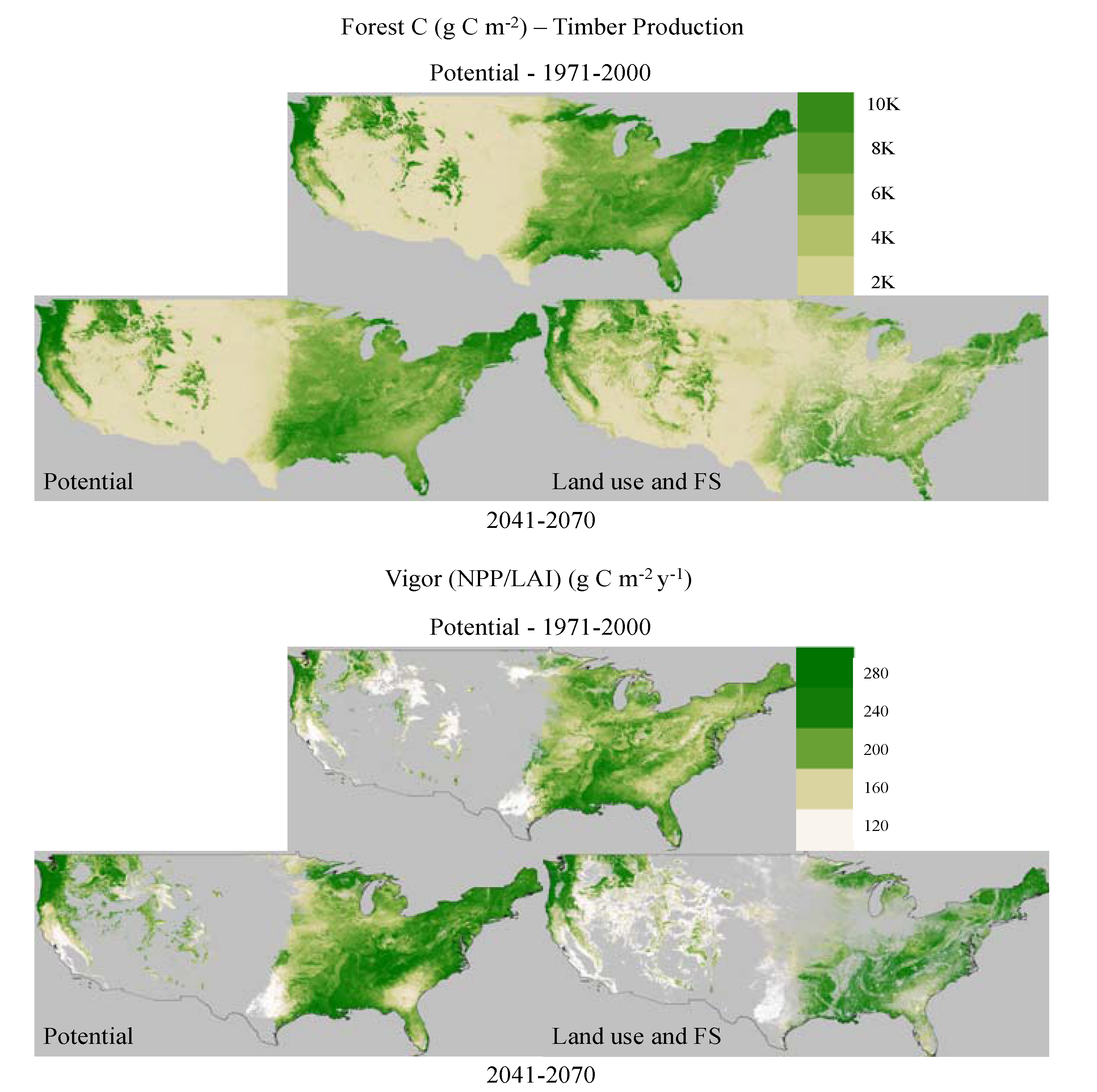
Figure 1. Simulated forest carbon stocks and forest vigor (NPP/LAI) for historical conditions (1971–2000) and for future conditions across 3 possible futures (climate projections from CGCM3, MIROC and CSIRO) under the A2 emission scenario (2041–2070). We show simulation results at 30 arcsec spatial resolution for mid-century with and without land use and fire suppression.
Climate 06 00001 g001
Figure 2. Simulated net ecosystem production (NEP), biomass consumed by wildfires and soil carbon for historical conditions (1971–2000) and for future conditions across 3 possible futures (climate projections from CGCM3, MIROC and CSIRO) under the A2 emission scenario (2041–2070). We show simulation results at 30 arcsec spatial resolution for mid-century with and without land use and fire suppression.
Climate 06 00001 g002
Figure 3. Simulated change in vegetation cover between historical conditions (1971–2000) and future conditions across 3 possible futures (climate projections from CGCM3, MIROC and CSIRO) under the A2 emission scenario (2041–2070). We show simulation results at 30 arcsec spatial resolution without fire suppression (potential vegetation)—changes are due only to climate effects, with only fire suppression—changes are due to both climate and suppression, with fire suppression and land use—changes are due to climate, fire suppression and land conversion.
Climate 06 00001 g003
Figure 4. Factors that may decrease the value of ecosystem services across the conterminous USA: a decrease in vigor (NPP/LAI) and the amount of biomass consumed by wildfires, comparing simulation results for mid-century conditions (2041–2070), with and without land use, across 3 possible futures (climate projections from CGCM3, MIROC and CSIRO) under the A2 emission scenario. Projected vigor is mapped where forest production is projected to be the highest and simulated carbon losses to wildfires are mapped where carbon sequestration is expected to be the greatest by mid-21st century. Simulation results were obtained by running the MC2 model at 30 arcsec spatial resolution.
Climate 06 00001 g004
Table 1. Simulated ecosystem services and their constraints for the conterminous USA using results from the MC2 model at 30 arcsec spatial resolution for the period 2041–2070 across 3 climate futures (CGCM3, CSIRO and MIROC) under the A2 emission scenario.
Total Area (Conterminous USA)Protected Areas (GAP 1 and 2)Managed Lands (ag/Grasslands, Developed, Mined)
Area7,873,389 km2609,235 km22,635,585 km2
Type of Human interventionnoneLand use + fire suppressionnonefire suppressionnoneLand use + fire suppression
Carbon sequestration-NEP (g∙C∙m−2)70.58154.6267.6371.4074.56325.24
Timber Supply (Gm 3 × 10⁶ km−2)20.0213.8821.99 123.64100.781.86
Biomass Consumed by wildfires (g∙C∙m−2)56.6822.5656.6338.4159.112.54
1 If timber was to be extracted from protected area. These are calculated only for comparison sake.