The Relationship between Atmospheric Carbon Dioxide Concentration and Global Temperature for the Last 425 Million Years


Abstract
1. Introduction
2. Methods
2.1. Data Sources
2.2. Temperature Proxies
2.3. CO2 Proxies
2.4. Analytic Approaches and Limitations
2.5. MODTRAN Computations
2.6. Pilot Studies
3. Results
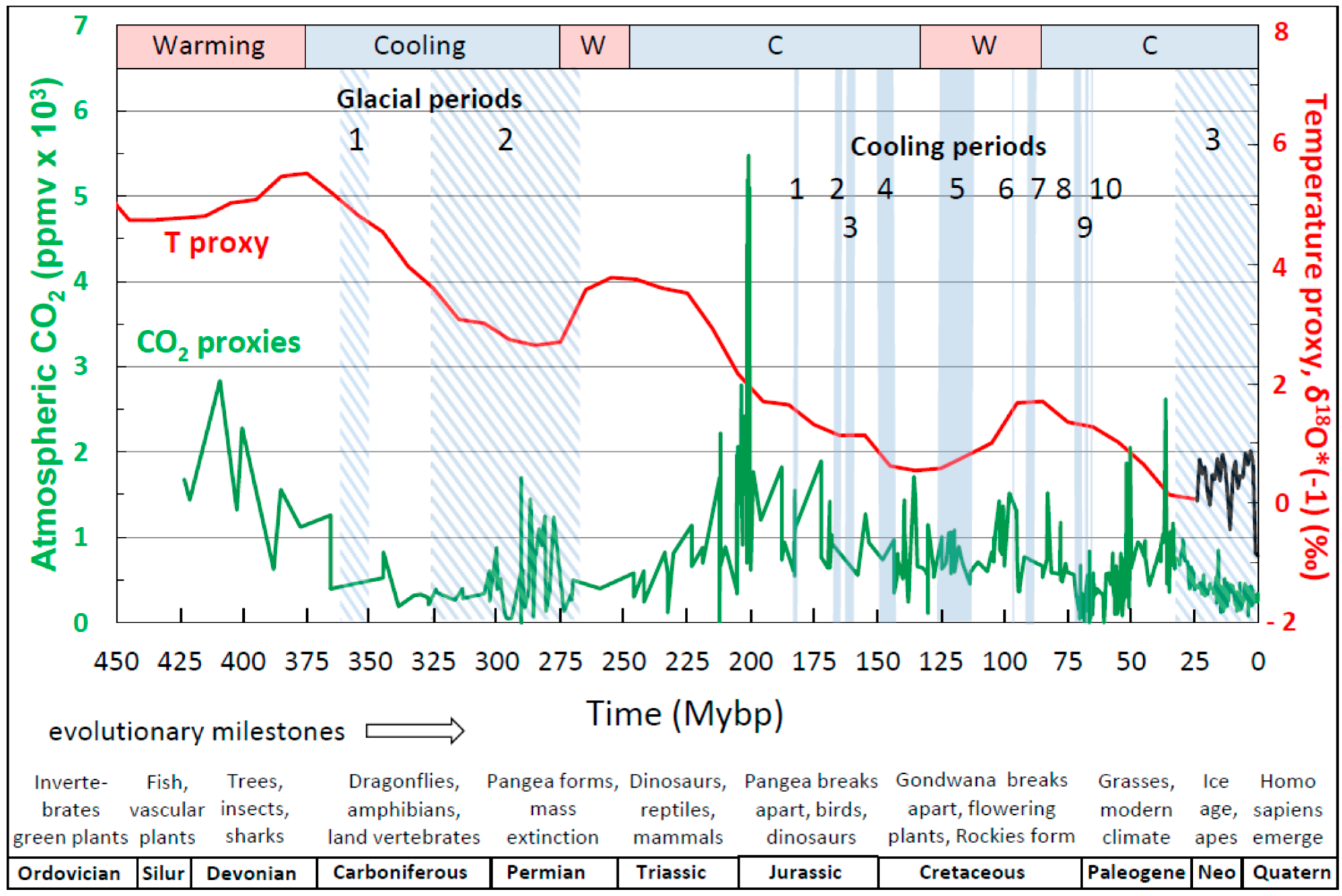
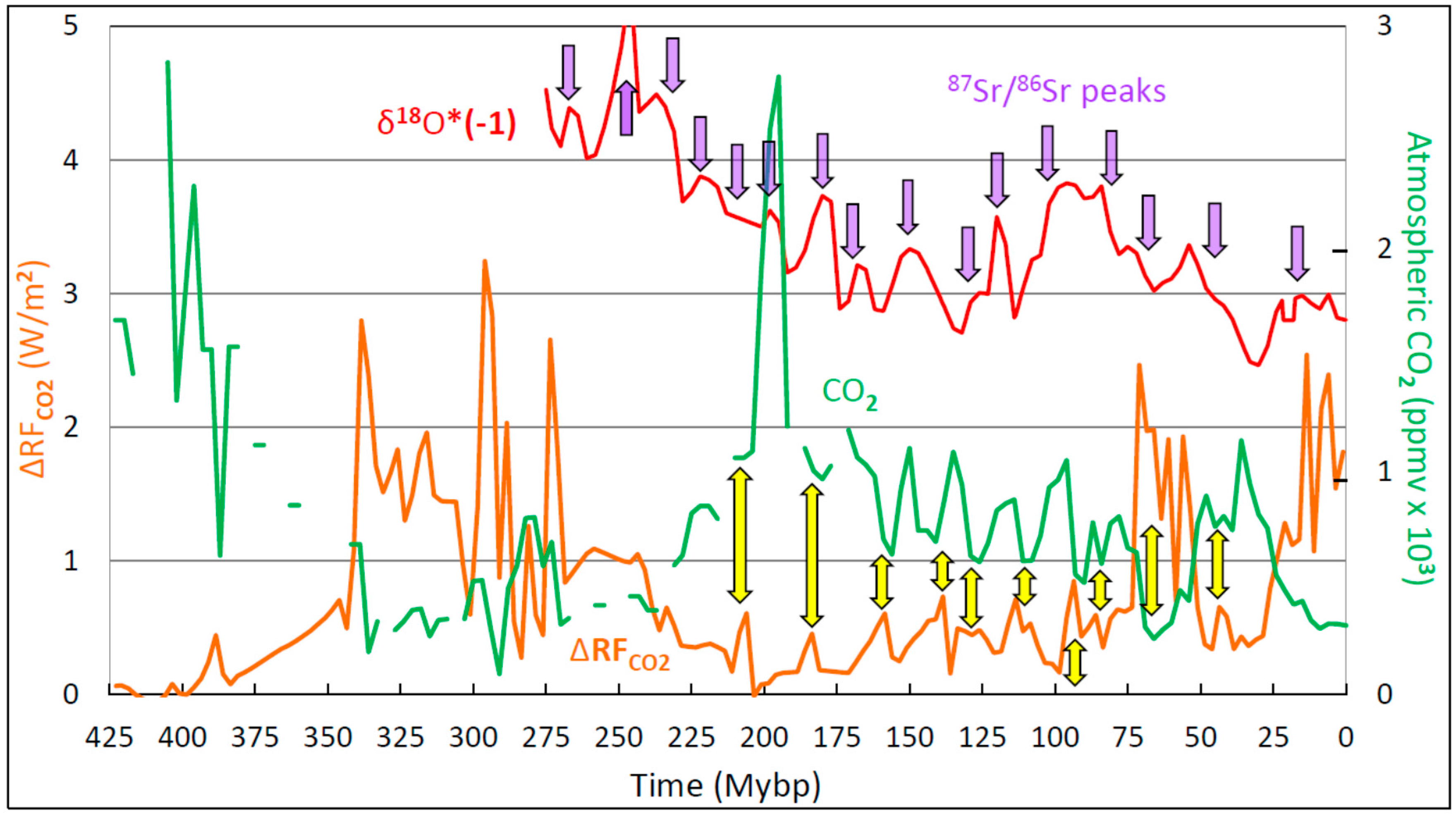
3.1. Overview of the Phanerozoic Climate
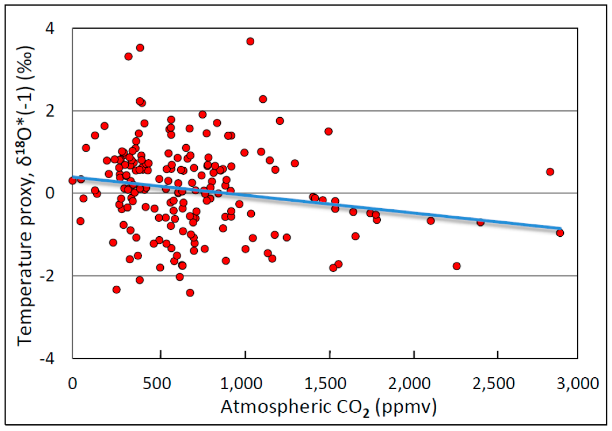
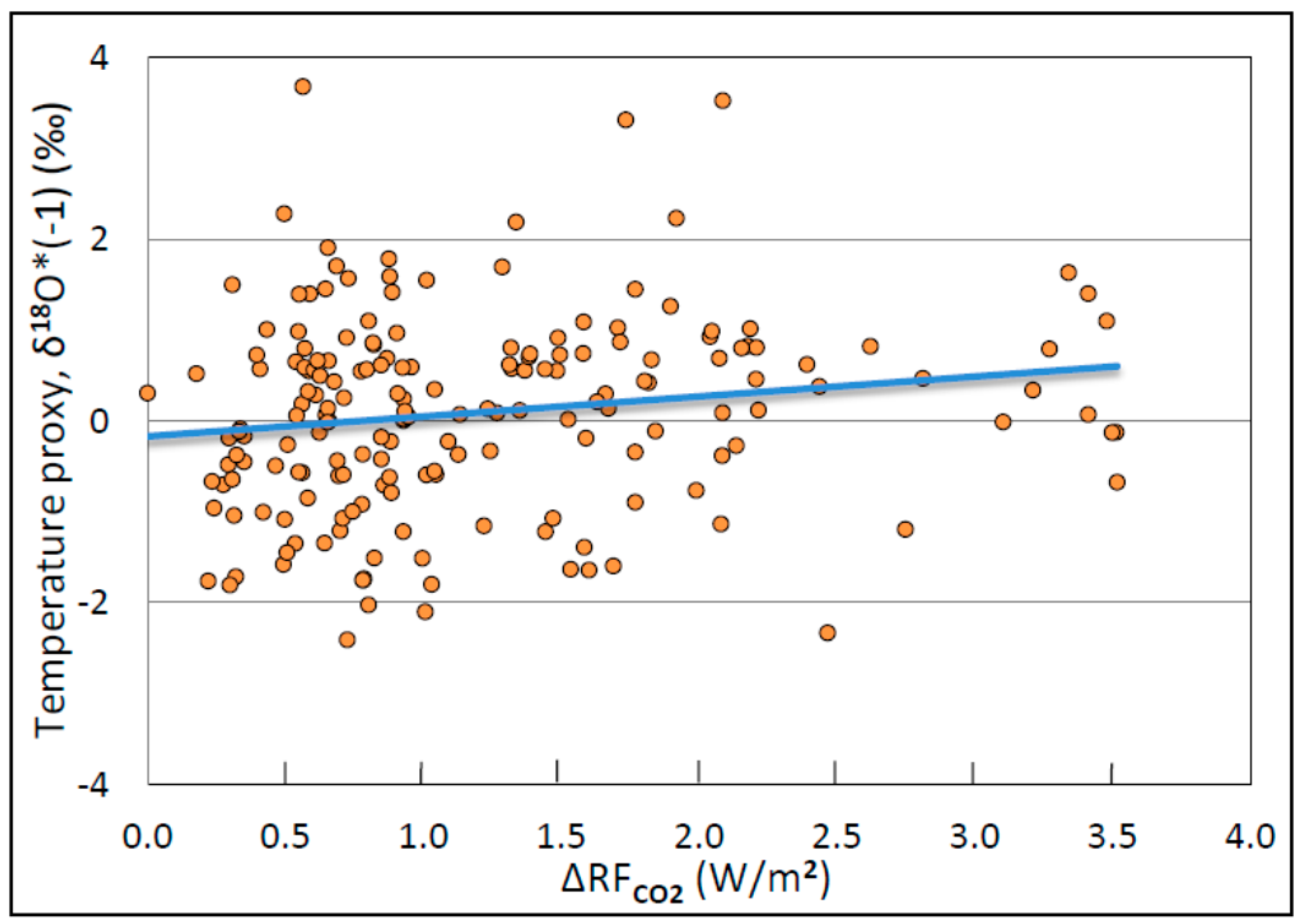
3.2. Temperature versus Atmospheric Carbon Dioxide
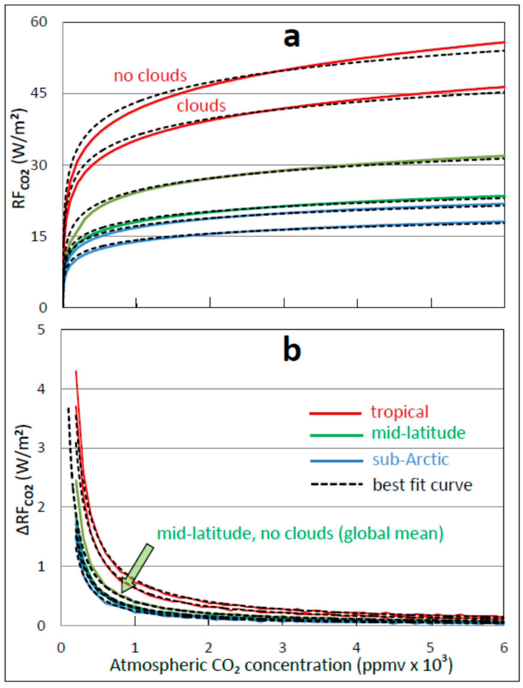
3.3. Marginal RF of Temperature by Atmospheric CO2
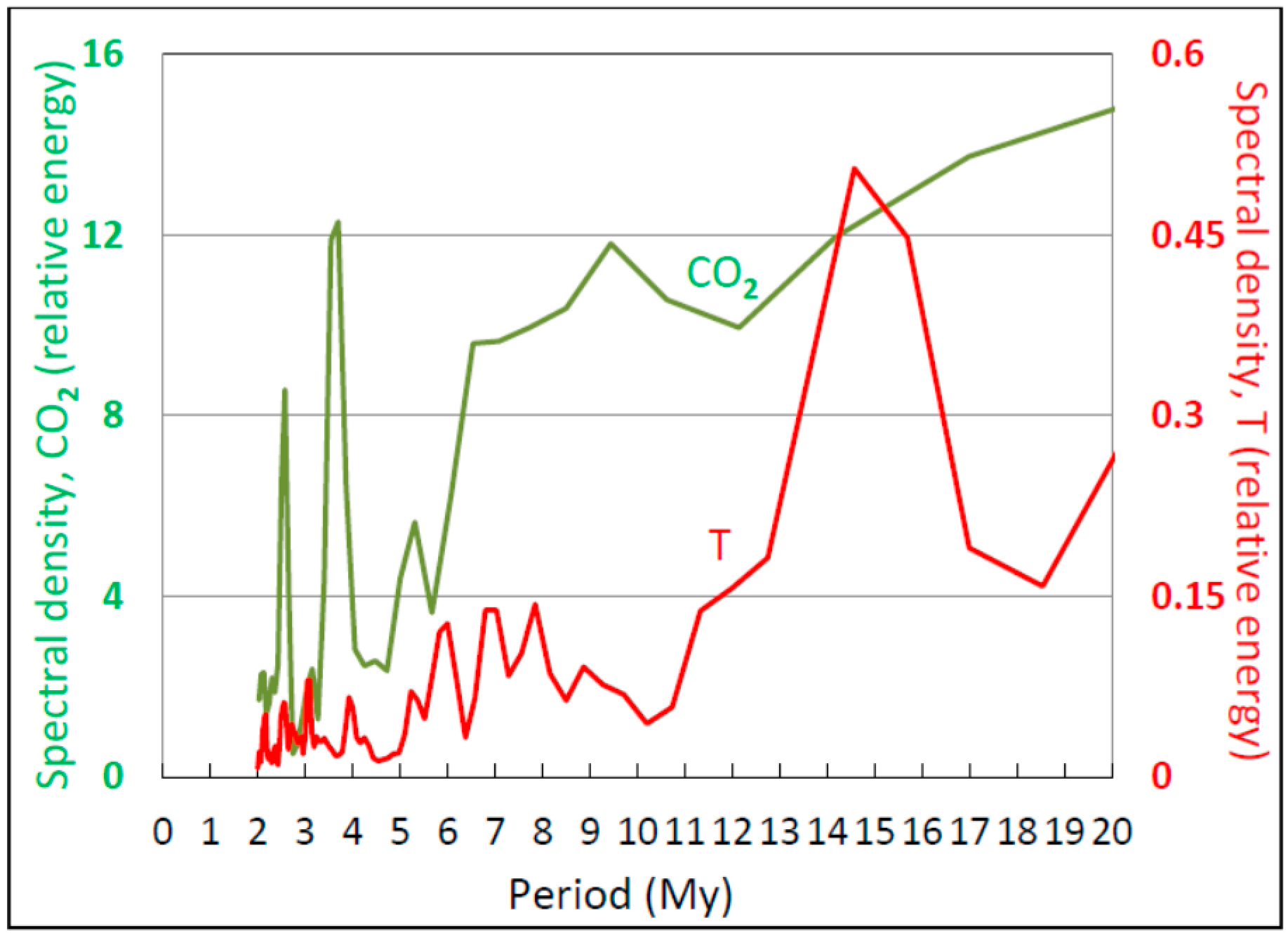
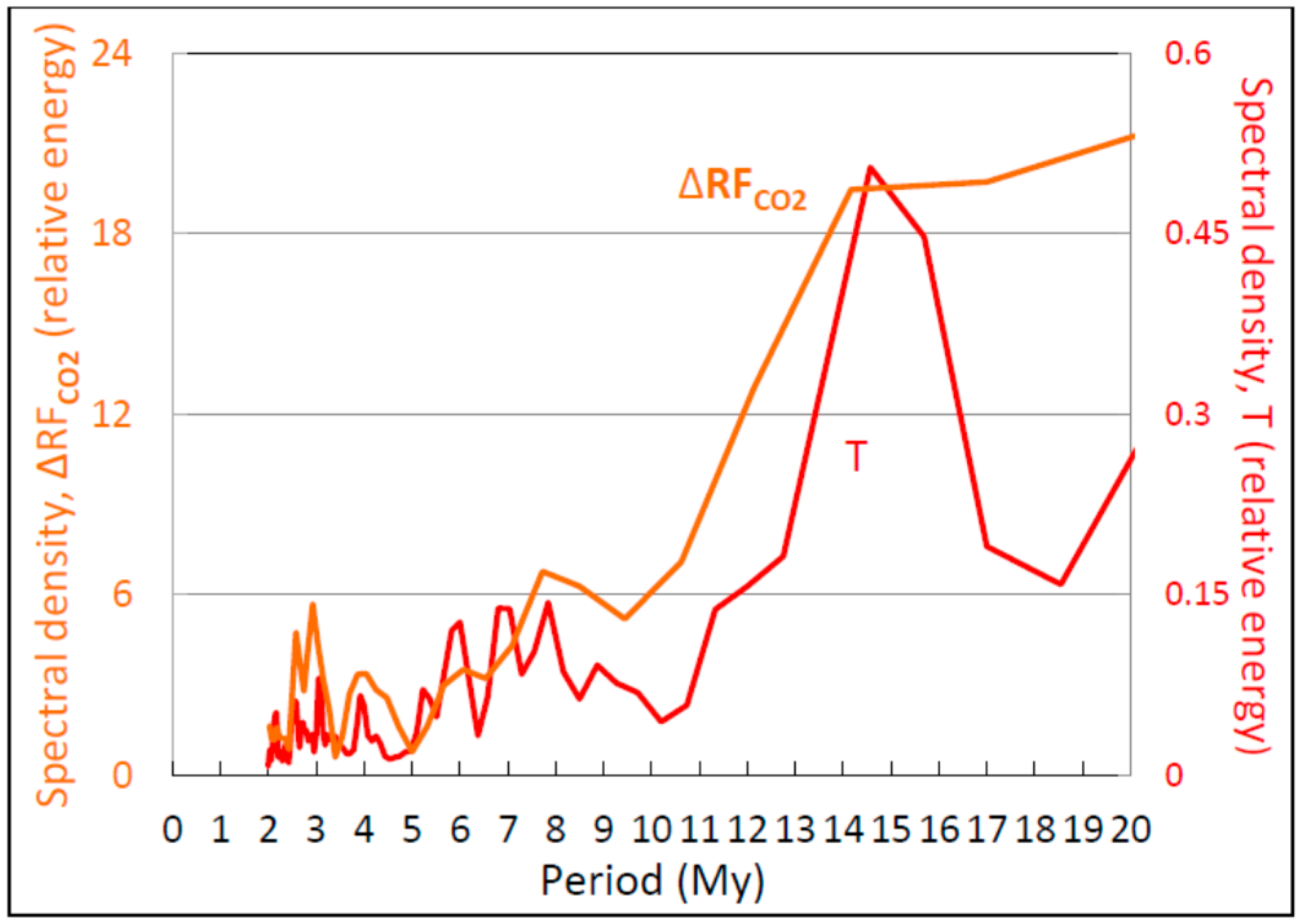
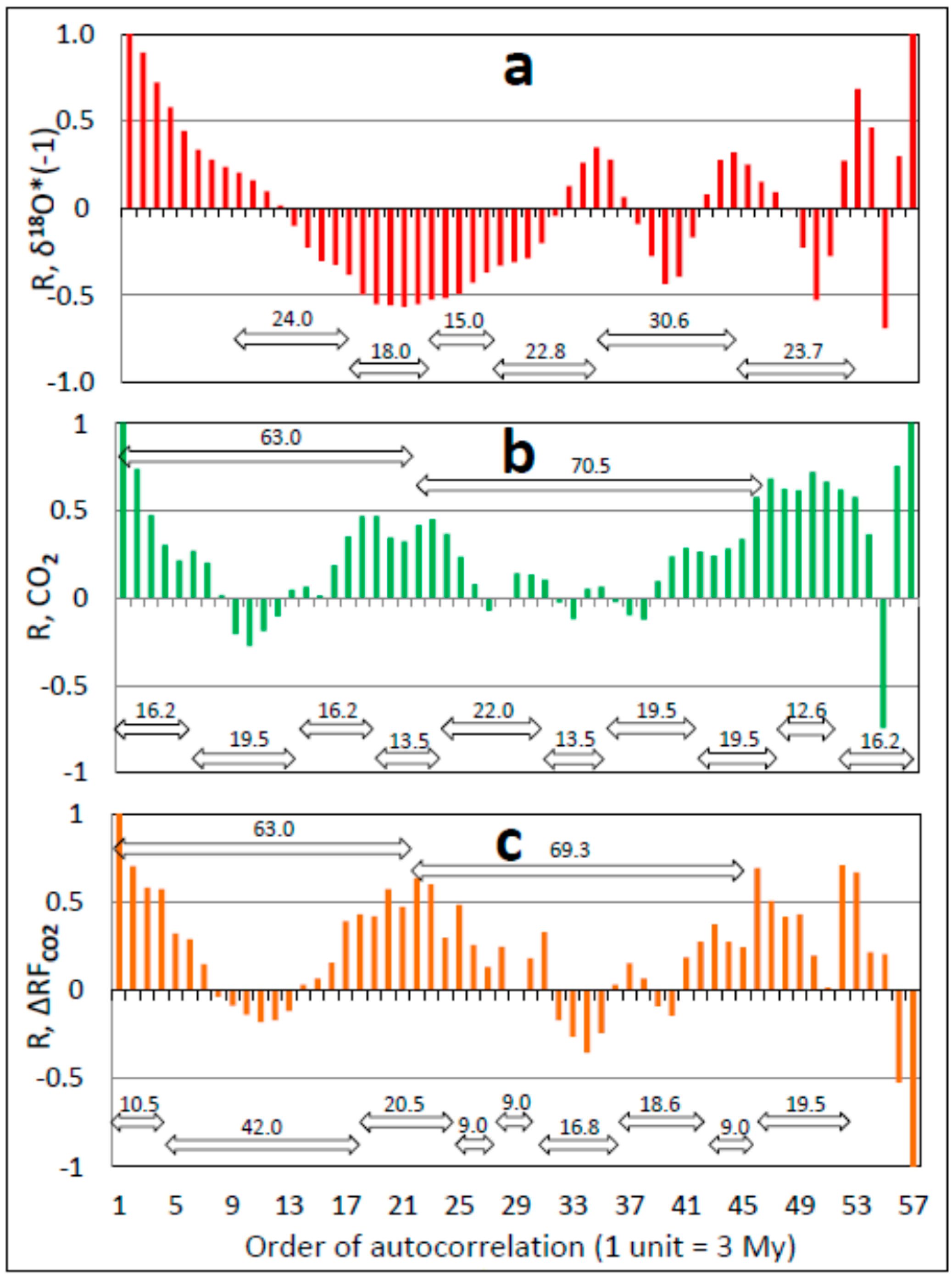
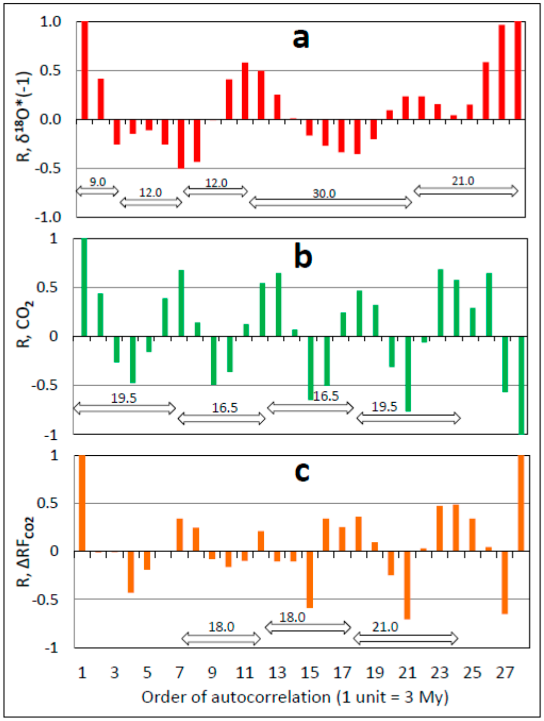
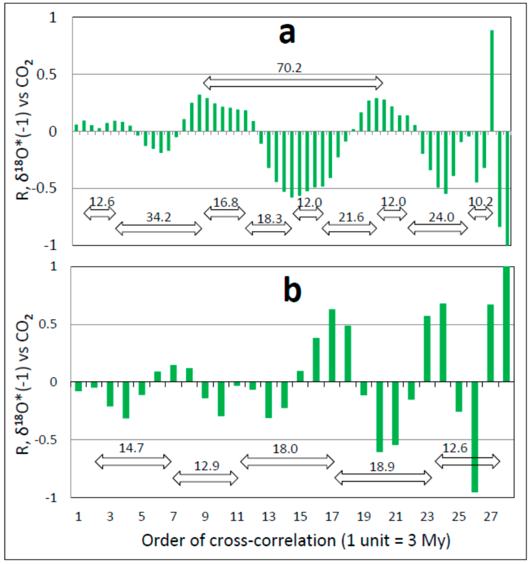
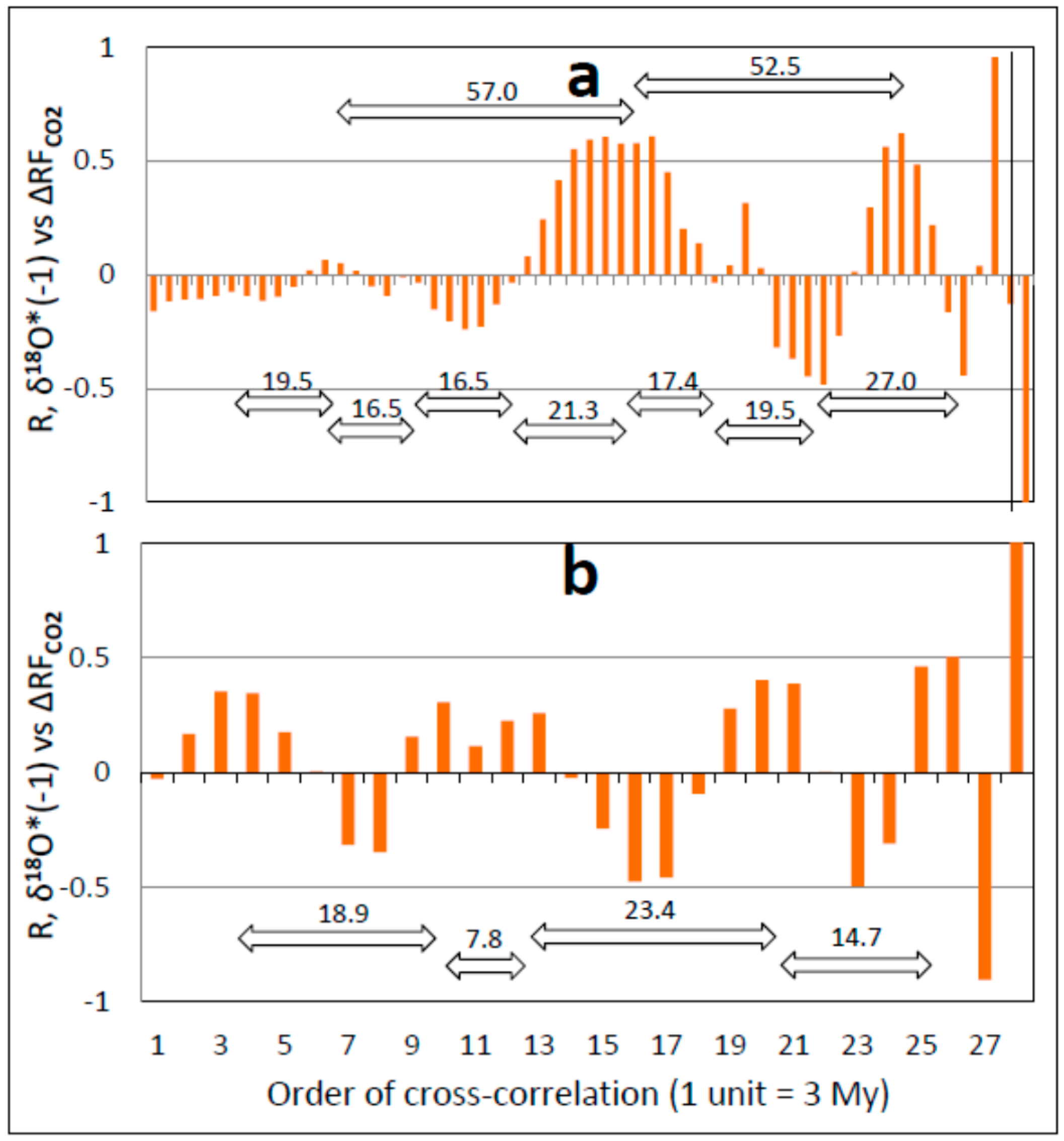
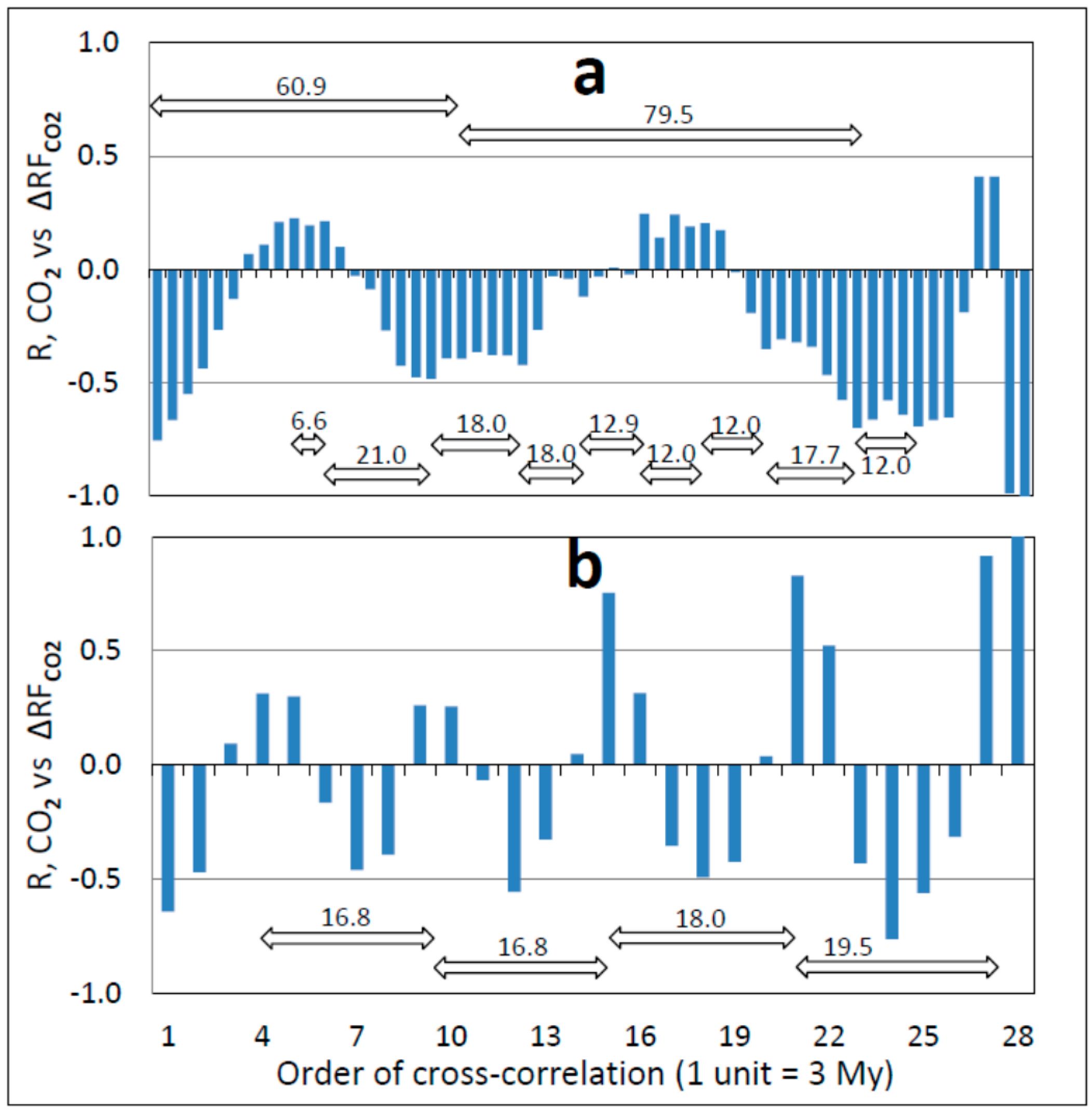
3.4. Auto- and Cross-Correlation
4. Discussion and Conclusions
4.1. Qualifications and Limitations
4.2. The Perspective of Previous Studies
4.3. Tectonic Activity and Climate in the Phanerozoic
4.4. The Physical Basis of CO2/T Decoupling
4.5. Implications for Glacial Cycling
4.6. Risk Assessment and Contemporary Carbon Policies
Acknowledgments
Conflicts of Interest
References
- Keeling, R.F.; Piper, S.C.; Bollenbacher, A.F.; Walker, J.S. Atmospheric CO2 records from sites in the SIO air sampling network. In Trends: A Compendium of Data on Global Change; Carbon Dioxide Information Analysis Center, Oak Ridge National Laboratory, U.S. Department of Energy: Oak Ridge, TN, USA, 2009. [Google Scholar] [CrossRef]
- NASA (National Aeronautic and Space Administration). 2017. Available online: http://earthobservatory.nasa.gov/Features/WorldOfChange/decadaltemp.php (accessed on 2 August 2017).
- Ramanathan, V. Trace-gas greenhouse effect and global warming: Underlying principles and outstanding issues. Ambio 1998, 17, 187–197. [Google Scholar]
- Peterson, T.C.; Connolley, W.M.; Fleck, J. The myth of the 1970s global cooling scientific consensus. Bull. Am. Meteorol. Soc. 2008, 89, 1325–1337. [Google Scholar] [CrossRef]
- Marsh, G.E. Interglacials, Milankovitch cycles, solar activity, and carbon dioxide. J. Climatol. 2014. [Google Scholar] [CrossRef]
- Fourier, J.B.J. Remarques générales sur les températures du globe terrestre et des espaces planétaires. Ann. Chim. Phys. 1824, 27, 136–167. [Google Scholar]
- Fourier, J.B.J. Mémoire sur la Température du Globe Terrestre et des Espaces Planétaires. Mém. Acad. R. Sci. 1827, 7, 569–604. [Google Scholar]
- Tyndall, J. On the absorption and radiation of heat by gases and vapours; on the physical connection of radiation, absorption, and conduction. Philos. Mag. 1861, 22, 273–285. [Google Scholar]
- Tyndall, J. On the passage of radiant heat through dry and humid air. Philos. Mag. 1863, 26, 44–54. [Google Scholar]
- Arrhenius, S. On the influence of carbonic acid in the air upon the temperature on the ground. Philos. Trans. 1896, 41, 237–276. [Google Scholar] [CrossRef]
- Callendar, G.S. The artificial production of carbon dioxide and its influence on temperature. Quart. J. R. Meteorol. Soc. 1938, 64, 223–240. [Google Scholar] [CrossRef]
- Plass, G. The influence of the 15μ carbon-dioxide band on the atmospheric infra-red cooling rate. Quart. J. R. Meteorol. Soc. 1956, 82, 310–324. [Google Scholar] [CrossRef]
- Adhémar, J.A. Révolutions de la Mer: Déluges Périodiques; Carilian-Goeury et V. Dalmont: Paris, France, 1842. [Google Scholar]
- Croll, J. Climate and Time in Their Geological Relations: A Theory of Secular Changes of the Earth’s Climate; Appleton: New York, NY, USA, 1890. [Google Scholar]
- Milankovitch, M. Mathematische Klimalehre und Astronomische Theorie der Klimaschwankungen. In Handbuch der Klimatologie; Koppen, W., Geiger, R., Eds.; Springer: Berlin, Germany, 1930; Volume 1, Part A. [Google Scholar]
- Revelle, R.; Broecker, W.; Craig, H.; Kneeling, C.D.; Smagorinsky, J. Restoring the Quality of Our Environment: Report of the Environmental Pollution Panel; President’s Science Advisory Committee: Washington, DC, USA, 1965; 317p. [Google Scholar]
- Charney, J.G.; Arakawa, A.; Baker, D.J.; Bolin, B.; Dickinson, R.E.; Goody, R.M.; Leith, C.E.; Stommel, H.M.; Wunsch, C.I. Carbon Dioxide and Climate: A Scientific Assessment; National Academy of Sciences USA: Washington, DC, USA, 1979. [Google Scholar]
- Crowley, T.J.; Berner, R.A. CO2 and climate change. Science 2001, 292, 870–872. [Google Scholar] [CrossRef] [PubMed]
- Royer, D.L.; Berner, R.A.; Montañez, I.P.; Tabor, N.J.; Beerling, D.J. CO2 as a primary driver of Phanerozoic climate. GSA Today 2004, 14, 4–10. [Google Scholar] [CrossRef]
- Royer, D.L.; Berner, R.A.; Park, J. Climate sensitivity constrained by CO2 concentrations over the past 420 million years. Nature 2007, 446, 530–532. [Google Scholar] [CrossRef] [PubMed]
- Royer, D.L. CO2-forced climate thresholds during the Phanerozoic. Geochim. Cosmochim. Acta 2006, 70, 5665–5675. [Google Scholar] [CrossRef]
- Frakes, L.A.; Francis, J.E. A guide to Phanerozoic cold polar climates from high-latitude ice-rafting in the Cretaceous. Nature 1988, 333, 547–549. [Google Scholar] [CrossRef]
- Frakes, L.A.; Francis, E.; Syktus, J.I. Climate Modes of the Phanerozoic: The History of the Earth’s Climate over the Past 600 Million Years; Cambridge University Press: Cambridge, UK, 1992; ISBN 0-521-36627-5. [Google Scholar]
- Veizer, J.; Godderis, Y.; François, L.M. Evidence for decoupling of atmospheric CO2 and global climate during the Phanerozoic Eon. Nature 2000, 408, 698–701. [Google Scholar] [CrossRef] [PubMed]
- Shaviv, N.J.; Veizer, J. Celestial driver of Phanerozoic climate? GSA Today 2003, 13, 4–10. [Google Scholar] [CrossRef]
- Boucot, A.J.; Gray, J.A. Critique of Phanerozoic climate models involving changes in the CO2 content of the atmosphere. Earth Sci. Rev. 2001, 56, 1–159. [Google Scholar] [CrossRef]
- Rothman, D.H. Atmospheric carbon dioxide levels for the last 500 million years. Proc. Natl. Acad. Sci. USA 2002, 99, 4167–4171. [Google Scholar] [CrossRef] [PubMed]
- Prokoph, A.; Shields, G.A.; Veizer, J. Compilation and time-series analysis of a marine carbonate δ18O, δ13C, 87Sr/86Sr and δ34S database through Earth history. Earth Sci. Rev. 2008, 87, 113–133. [Google Scholar] [CrossRef]
- IPCC (Intergovernmental Panel on Climate Change). Climate Change 2001: The Scientific Basis; Houghton, J.T., Ed.; Cambridge University Press: New York, NY, USA, 2001. [Google Scholar]
- IPCC (Intergovernmental Panel on Climate Change). Climate Change 2007: The Physical Science Basis; Contribution of Working Group I to the Fourth Assessment Report of the Intergovernmental Panel on Climate Change; Solomon, S., Ed.; Cambridge University Press: New York, NY, USA, 2007. [Google Scholar]
- IPCC (Intergovernmental Panel on Climate Change). Climate Change 2013: The Physical Science Basis; Contribution of Working Group I to the Fifth Assessment Report of the Intergovernmental Panel on Climate Change; Stocker, T.F., Ed.; Cambridge University Press: New York, NY, USA, 2013. [Google Scholar]
- Lacis, A.A.; Schmidt, G.A.; Rind, D.; Rudy, R.A. Atmospheric CO2: Principal control knob governing earth’s temperature. Science 2010, 330, 356–359. [Google Scholar] [CrossRef] [PubMed]
- Hoerling, M.; Eischeid, J.; Kumar, A.; Leung, R.; Mariotti, A.; Mo, K.; Schubert, S.; Seager, R. Causes and predictability of the 2012 Great Plains drought. Bull. Am. Meteorol. Soc. 2014, 95L, 269–282. [Google Scholar] [CrossRef]
- Schubert, S.; Gutzler, D.; Wang, H.; Dai, A.; Delworth, T.; Deser, C.; Findell, K.; Fu, R.; Higgens, W.; Hoerling, M.; et al. CLIVAR project to assess and compare the responses of global climate models to drought-related SST forcing patterns: Overview and results. J. Clim. 2009, 22, 5251–5272. [Google Scholar] [CrossRef]
- Findell, K.L.; Delworth, T.L. Impact of common sea surface temperature anomalies on global drought and pluvial frequency. J. Clim. 2010, 23, 485–503. [Google Scholar] [CrossRef]
- Kushnir, Y.; Seager, R.; Ting, M.; Naik, N.; Nakamura, J. Mechanisms of tropical Atlantic influence on North American hydroclimate variability. J. Clim. 2010, 23, 5610–5628. [Google Scholar] [CrossRef]
- Chang, C.-P.; Ghil, M.; Kuo, H.-C.; Latif, M.; Sui, C.-H.; Wallace, J.M. Understanding multidecadal climate changes. Bull. Am. Meteorol. Soc. 2014, 95, 293–296. [Google Scholar] [CrossRef]
- Veizer, J.; Ala, D.; Azmy, K.; Bruckschen, P.; Buhl, D.; Bruhn, F.; Carden, G.A.F.; Diener, A.; Ebneth, S.; Godderis, Y.; et al. 87Sr/86Sr, δ13C and δ18O evolution of Phanerozoic seawater. Chem. Geol. 1999, 161, 59–88. [Google Scholar] [CrossRef]
- Veizer, J.; Prokoph, A. Temperature and oxygen isotopic composition of Phanerozoic oceans. Earth Sci. Rev. 2015, 146, 92–104. [Google Scholar] [CrossRef]
- Royer, D.L. Atmospheric CO2 and O2 during the Phanerozoic: Tools, patterns and impacts. In Treatise on Geochemistry, 2nd ed.; Holland, H., Turekian, K., Eds.; Elselvier: Amsterdam, The Netherlands, 2014; pp. 251–267. [Google Scholar]
- Jouzel, J. Calibrating the isotopic paleothermometer. Science 1999, 286, 910–911. [Google Scholar] [CrossRef]
- Nagornov, O.V.; Konovalov, Y.V.; Tchijov, V. Temperature reconstruction for Arctic glaciers. Paleogeog. Paleoclim. Paleoecol. 2006, 236, 125–134. [Google Scholar] [CrossRef]
- Masson-Delmotte, V.; Hou, S.; Ekaykin, A.; Jouzel, J.; Aristariain, A.; Bernardo, R.T.; Bromwich, D.; Cattani, O.; Delmotte, M.; Falourd, S.; et al. A review of Antarctic surface snow isotopic composition: Observations, atmospheric circulation, and isotopic modeling. J. Clim. 2008, 21, 3359–3387. [Google Scholar] [CrossRef]
- Grossman, E.L. Applying oxygen isotope paleothermometry in deep time. Paleontol. Soc. Pap. 2012, 18, 39–68. [Google Scholar] [CrossRef]
- Lécuyer, C.; Amiot, R.; Touzeau, A.; Trotter, J. Calibration of the phosphate δ18O thermometer with carbonate-water oxygen isotope fractionation equations. Chem. Geol. 2013, 347, 217–226. [Google Scholar] [CrossRef]
- Lee, J.-E.; Fung, I.; DePaolo, J.; Otto-Bliesner, B. Water isotopes during the Last Glacial Maximum: New general circulation model calculations. J. Geophys. Res. Atmos. 2008. [Google Scholar] [CrossRef]
- Demény, A.; Kele, S.; Siklósy, Z. Empirical equations for the temperature dependence of calcite-water oxygen isotope fractionation from 10 to 70 °C. Rapid Commun. Mass Spectrom. 2010, 24, 3521–3526. [Google Scholar] [CrossRef] [PubMed]
- Myhre, G.; Highwood, E.J.; Shine, K.P. New estimates of radiative forcing due to well mixed greenhouse gases. Geophys. Res. Lett. 1998, 25, 2715–2718. [Google Scholar] [CrossRef]
- Pearson, P.N.; Palmer, M.R. Atmospheric carbon dioxide concentrations over the past 60 million years. Nature 2000, 406, 695–699. [Google Scholar] [CrossRef] [PubMed]
- Pearson, P.N.; Ditchfield, P.W.; Singano, J.; Harcourt-Brown, K.G.; Nicholas, C.J.; Olsson, R.K.; Shackleton, N.J.; Hall, M.A. Warm tropical sea surface temperatures in the Late Cretaceous and Eocene epochs. Nature 2001, 413, 481–487. [Google Scholar] [CrossRef] [PubMed]
- Edgar, K.M.; Pälike, H.; Wilson, P.A. Testing the impact of diagenesis on the δ18O and δ13C of benthic foraminiferal calcite from a sediment burial depth transect in the equatorial Pacific. Palaeoceanog. 2013, 28, 468–480. [Google Scholar] [CrossRef]
- Anagnostou, E.; John, E.H.; Edgar, K.M.; Foster, G.L.; Ridgwell, A.; Inglis, G.N.; Pancost, R.D.; Lunt, D.J.; Pearson, P.N. Changing atmospheric CO2 concentration was the primary driver of early Cenozoic climate. Nature 2016, 533, 380–384. [Google Scholar] [CrossRef] [PubMed]
- Nyquist, H. Certain topics in telegraph transmission theory. AIEEE 1928, 47, 617–644. [Google Scholar] [CrossRef]
- Shannon, C.E. Communication in the presence of noise. Proc. IRE 1949, 37, 10–21. [Google Scholar] [CrossRef]
- Jerri, A.J. The Shannon Sampling Theorem—Its various extensions and applications: A tutorial review. Proc. IEEE 1977, 65, 1565–1596. [Google Scholar] [CrossRef]
- Landau, H.J. Necessary density conditions for sampling and interpolation of certain entire functions. Acta Math. 1967, 117, 37–52. [Google Scholar] [CrossRef]
- Collins, W.D.; Ramaswamy, V.; Schwarzkopf, M.D.; Sun, Y.; Portmann, R.W.; Fu, Q.; Casanova, S.E.B.; Dufresne, J.-L.; Fillmore, D.W.; Forster, P.M.D.; et al. Radiative forcing by well-mixed greenhouse gases: Estimates from climate models in the Intergovernmental Panel on Climate Change (IPCC) Fourth Assessment Report (AR4). J. Geophys. Res. Atmos. 2006, 111. [Google Scholar] [CrossRef]
- Driggers, R.G.; Friedman, M.H.; Nicols, J.M. An Introduction to Infrared and Electro-Optical Systems, 2nd ed.; Artech House: London, UK, 2012; ISBN 13:978-1-60807-100-5. [Google Scholar]
- MODTRAN Infrared Light in the Atmosphere. Available online: http://forecast.uchicago.edu/modtran.html (accessed on 23 September 2017).
- Petit, J.R.; Jouzel, J.; Raynaud, D.; Barkov, N.I.; Barnola, J.M.; Basile, I.; Bender, M.; Chappellaz, J.; Davis, J.; Delaygue, G.; et al. Climate and atmospheric history of the past 420,000 years from the Vostok ice core, Antarctica. Nature 1999, 399, 429–436. [Google Scholar] [CrossRef]
- Jouzel, J.; Masson-Delmotte, V.; Cattani, O.; Dreyfus, G.; Falourd, S.; Hoffmann, G.; Minster, B.; Nouet, J.; Barnola, J.M.; Chappellaz, J.; et al. Orbital and millennial Antarctic climate variability over the past 800,000 years. Science 2007, 317, 793–797. [Google Scholar] [CrossRef] [PubMed]
- Parrish, J.T. Interpreting Pre-Quaternary Climate from the Geologic Record; Columbia University: New York, NY, USA, 1998. [Google Scholar]
- Tufte, E.R. The Cognitive Style of PowerPoint; Graphics Press: Cheshire, CT, USA, 2003; Volume 2006. [Google Scholar]
- Came, R.E.; Eller, J.M.; Veizer, J.; Azmy, K.; Brand, U.; Weldman, C.R. Coupling of surface temperatures and atmospheric CO2 concentrations during the Paleozoic era. Nature 2007, 449, 198–201. [Google Scholar] [CrossRef] [PubMed]
- Zachos, J.; Pagani, M.; Sloan, L.; Thomas, E.; Billups, K. Trends, rhythms, and aberrations in global climate 65 Ma to present. Science 2001, 292, 686–693. [Google Scholar] [CrossRef] [PubMed]
- Lisiecki, L.E.; Raymo, M.E. A Pliocene-Pleistocene stack of 57 globally distributed benthic δ18O records. Paleocean 2005, 20, 1003–1020. [Google Scholar] [CrossRef]
- Foster, G.L.; Royer, D.L.; Lunt, D.J. Future climate forcing potentially without precedent in the last 420 million years. Nat. Commun. 2017, 8, 14845. [Google Scholar] [CrossRef] [PubMed]
- Franks, P.J.; Royer, D.L.; Beerling, D.J.; Van de Water, P.K.; Cantrill, D.J.; Barbour, M.; Berry, J.A. New constraints on atmospheric CO2 concentration for the Phanerozoic. Geophys. Res. Lett. 2014, 41, 4685–4694. [Google Scholar] [CrossRef]
- Vérard, C.; Hochard, C.; Baumgartner, P.O.; Stampfli, G.M.; Liu, M. Geodynamic evolution of the Earth over the Phanerozoic: Plate tectonic activity and paleoclimatic indicators. J. Paleogeog. 2015, 4, 167–188. [Google Scholar] [CrossRef]
- Raymo, M.E.; Ruddiman, W.F. Tectonic forcing of late Cenozoic climate. Nature 1992, 359, 117–122. [Google Scholar] [CrossRef]
- Gordon, L.I.; Jones, L.B. The effect of temperature on carbon dioxide partial pressures in seawater. Mar. Chem. 1973, 1, 317–322. [Google Scholar] [CrossRef]
- Weiss, R.F. Carbon dioxide in water and seawater: The solubility of a non-ideal gas. Mar. Chem. 1974, 2, 203–215. [Google Scholar] [CrossRef]
- Sigman, D.M.; Hain, M.P.; Haug, G.M. The polar ocean and glacial cycles in atmospheric CO2 concentration. Nature 2010, 466, 47–55. [Google Scholar] [CrossRef] [PubMed]
- Caldeira, K.; Kasting, J.F. Insensitivity of global warming potentials to carbon dioxide emission scenarios. Nature 1993, 366, 251–253. [Google Scholar] [CrossRef]
- Van der Pol, B. A theory of the amplitude of free and forced triode vibrations. Rad. Rev. 1920, 1, 701–710, 754–762. [Google Scholar]
- Lorenz, E.N. Deterministic non-periodic flow. J. Atmos. Sci. 1963, 20, 130–141. [Google Scholar] [CrossRef]
- Källén, E.; Crafoord, C.; Ghil, M. Free oscillations in a climate model with ice-sheet dynamics. J. Atmos. Sci. 1979, 36, 2292–2393. [Google Scholar] [CrossRef]
- Ghil, M.; Le Treut, H. A climate model with cryodynamics and geodynamics. J. Geophys. Res. Oceans 1981, 86, 5262–5270. [Google Scholar] [CrossRef]
- Yiou, P.; Ghil, M.; Jouzel, J.; Paillard, D.; Vautard, R. Nonlinear variability of the climatic system from singular and power spectra of Late Quaternary records. Clim. Dyn. 1994, 9, 371–389. [Google Scholar] [CrossRef]
- Paillard, D. Glacial cycles: Toward a new paradigm. Rev. Geophys. 2001, 39, 325–346. [Google Scholar] [CrossRef]
- Crucifix, M. Oscillators and relaxation phenomena in Pleistocene climate theory. Philos. Trans. Roy. Soc. A 2012, 370, 1140–1165. [Google Scholar] [CrossRef] [PubMed]
- Schmalensee, R. Comparing greenhouse gases for policy purposes. Energy J. 1993, 14, 245–255. [Google Scholar] [CrossRef]
- Den Elzen, M.; Schaeffer, M. Responsibility for past and future global warming: Uncertainties in attributing anthropogenic climate change. Clim. Chang. 2002, 54, 29–73. [Google Scholar] [CrossRef]
- Toi, R.J. The marginal costs of greenhouse gas emissions. Energy J. 1999, 20, 61–81. [Google Scholar]
- Den Elzen, M.; Fuglestvedt, J.; Höhne, N.; Trudinger, C.; Lowe, J.; Matthewsf, B.; Romstad, B.; Pires de Campos, C.; Andronova, N. Analyzing countries’ contribution to climate change: Scientific and policy-related choices. Environ. Sci. Policy 2005, 8, 614–636. [Google Scholar] [CrossRef]
- Doney, S.C.; Fabry, V.J.; Feely, R.A.; Kleypas, J.A. Ocean acidification: The other CO2 problem. Ann. Rev. Mar. Sci. 2009, 1, 169–192. [Google Scholar] [CrossRef] [PubMed]
- Weinbauer, M.G.; Mari, X.; Gattuso, J.-P. Effects of ocean acidification on the diversity and activity of heterotrophic marine microorganisms. In Ocean Acidification; Gattuso, J.-P., Hansson, L., Eds.; Oxford University Press: New York. NY, USA, 2012; pp. 83–98. ISBN 978-0-19-959108-4. [Google Scholar]
- Bambach, R.K. Phanerozoic biodiversity mass extinctions. Ann. Rev. Earth Planet. Sci. 2006, 34, 127–155. [Google Scholar] [CrossRef]
- Raup, D.M.; Sepkoski, J.J. Periodicity of extinctions in the geologic past. Proc. Natl. Acad. Sci. USA 1984, 81, 801–805. [Google Scholar] [CrossRef] [PubMed]
- Rhode, R.A.; Muller, R.A. Cycles in fossil diversity. Nature 2005, 434, 208–210. [Google Scholar] [CrossRef] [PubMed]
- Archer, D.; Eby, M.; Brovkin, V.; Ridgwell, A.; Long, C.; Mikolajewicz, U.; Caldeira, K.; Matsumoto, K.; Munhoen, G.; Montenegro, A.; et al. Atmospheric lifetime of fossil fuel carbon dioxide. Annu. Rev. Earth Planet. Sci. 2009, 37, 117–134. [Google Scholar] [CrossRef]
- Archer, D.; Kheshgi, H.; Maier-Riemer, E. Multiple time scales for neutralization of fossil fuel CO2. Geophys. Res. Lett. 1997, 24, 405–408. [Google Scholar] [CrossRef]
- Galgani, L.; Stolle, C.; Endres, S.; Schulz, K.; Engel, A. Effects of ocean acidification on the biogenic composition of the sea-surface microlayer: Results from a mesocosm study. J. Geophys. Res. 2014. [Google Scholar] [CrossRef]


| A. Entry # | B. Time (Mybp) | C. Geological Periods and/or Description | D: R (n, p) | |
|---|---|---|---|---|
| D(1): CO2 v. T | D(2): ΔRFCO2 v. T | |||
| 1 | 71.6–69.6 | Campanian-Maastrichtian boundary | a N/A | a N/A |
| b N/A | b N/A | |||
| c 0.31 (19, 0.19) | c −0.31 (19, 0.20) | |||
| d −0.20 (11, 0.56) | d 0.02 (11, 0.96) | |||
| e −0.39 (11, 0.23) | e 0.39 (11, 0.23) | |||
| 2 | 80–50 | bracketed Campanian-Maastrichtian boundary | a 0.16 (31, 0.40) | a −0.06 (31, 0.75) |
| b 0.16 (31, 0.38) | b −0.05 (31, 0.80) | |||
| a 0.17 (31, 0.35) | a −0.12 (31, 0.52) | |||
| b 0.19 (31, 0.31) | b −0.12 (31, 0.52) | |||
| d 0.03 (110, 0.78) | d −0.13 (110, 0.19) | |||
| e −0.006 (110, 0.95) | e 0.03 (110, 0.72) | |||
| 3 | 67.5–66.5 | mid-Maastrichtian | a N/A | a N/A |
| b N/A | b N/A | |||
| c 0.09 (17, 0.92) | c −0.02 (17, 0.93) | |||
| d N/A | d N/A | |||
| e N/A | e N/A | |||
| 4 | 80–40 | bracketed mid-Maastrichtian | a −0.11 (41, 0.48) | a 0.14 (41, 0.37) |
| b 0.01 (41, 0.95) | b 0.06 (41, 0.70) | |||
| a −0.16 (41, 0.32) | a 0.10 (41, 0.55) | |||
| b 0.002 (41, 0.99) | b −0.03 (41, 0.84) | |||
| d −0.004 (116, 0.96) | d −0.12 (116, 0.20) | |||
| e −0.04 (116, 0.68) | e 0.05 (116. 0.59) | |||
| 5 | 0–34 | most recent global glaciation (late Cenozoic) | a −0.63 (34, 0.00005) | a 0.63 (34, 0.001) |
| b −0.73 (34, 0.00001) | b 0.53 (34, 0.00006) | |||
| a −0.48 (34, 0.0041) | a 0.52 (34, 0.002) | |||
| b −0.58 (34, 0.0003) | b 0.62 (34, 0.0001) | |||
| d −0.25 (179, 0.0006) | d 0.20 (179, 0.0075) | |||
| e −0.26 (179, 0.0005) | e 0.26 (179, 0.0005) | |||
| 6 | 0–26 | late Cenozoic, CO2 range similar to present | a 0.043 (26, 0.83) | a −0.02 ( 26, 0.94) |
| b −0.16 (26, 0.44) | b 0.16 (26, 0.42) | |||
| a −0. 052 (26, 0.80) | a 0.12 (26, 0.55) | |||
| b −0.16 (26, 0.44) | b 0.23 (26, 0.25) | |||
| d −0.03 (154, 0.70) | d 0.03 (154, 0.71) | |||
| e −0.05 (154, 0.53) | e 0.05 (154, 0.53) | |||
| A. Entry # | B. Time (Mybp) | C. Geological Periods Covered and/or Description | D: R (n, p) | |
|---|---|---|---|---|
| D(1): CO2 v. T | D(2): ΔRFCO2 v. T | |||
| 1 | 0–424 | most of Phanerozoic Eon | a 0.15 (191, 0.035) | a 0.10 (185, 0.16) |
| b −0.19 (206, 0.006) | b 0.16 (199, 0.02) | |||
| a −0.048 (191, 0.248) | a −0.037 (185, 0.61) | |||
| b −0.202 (191, 0.005) | b 0.193 (185, 0.0082) | |||
| 2 | 424–285 | first Phanerozoic temperature cycle (trough to trough) | a 0.22 (33, 0.23) | a −0.14 (35, 0.42) |
| b −0.16 (33, 0.37) | b 0.17 (35, 0.32) | |||
| a −0.04 (33, 0.86) | a 0.28 (33, 0.21) | |||
| b −0.095 (33, 0.61) | b 0.17 (33, 0.36) | |||
| 3 | 285–135 | second Phanerozoic temperature cycle (trough to trough) | a −0.17 (43, 0.26) | a 0.33 (39, 0.04) |
| b −0.16 (43, 0.30) | b 0.25 (39, 0.12) | |||
| a −0.14 (43, 0.36) | a 0.18 (39, 0.28) | |||
| b −0.22 (38, 0.10) | b 0.19 (38, 0.23) | |||
| 4 | 326–267 | Permo-Carboniferous glaciation | a 0.28 (22, 0.28) | a 0.03 (21, 0.90) |
| b 0.28 (22, 0.20) | b 0.05 (21, 0.82) | |||
| a 0.09 (22, 0.69) | a 0.26 (21, 0.25) | |||
| b −0.03 (20, 0.90) | b 0.26 (20, 0.27) | |||
| 5 | 400–200 | bracketed Permo-Carboniferous glaciation | a −0.30 (44, 0.05) | a 0.20 (42, 0.20) |
| b −0.17 (44, 0.26) | b 0.16 (42, 0.31) | |||
| a −0.22 (44, 0.16) | a 0.31 (42, 0.04) | |||
| b −0.12 (44, 0.44) | b 0.24 (42, 0.12) | |||
| 6 | 225–73 | Period of flat baseline with ~My ΔRF oscillations | a 0.15 (80, 0.17) | a −0.10 (70, 0.28) |
| b −0.11 ( 80, 0.25) | b −0.10 (77, 0.38) | |||
| a 0.23 (76, 0.042) | a −0.27 (72, 0.02) | |||
| b −0.03 (76, 0.79) | b −0.01 (70, 0.93) | |||
| 7 | 184–66.5 | early Jurassic to Cretaceous (brackets all cool periods) | a 0.15 (71, 0.11) | a −0.24 (68, 0.03) |
| b −0.01 (71, 0.09) | b −0.05 (68, 0.68) | |||
| a 0.20 (71, 0.09) | a −0.25 (68, 0.04) | |||
| b 0.02 (71, 0.88) | b −0.07 (68, 0.56) | |||
| 8 | 200–50 | bracketed early Jurassic to Cretaceous | a 0.21 (93, 0.02) | a −0.21 (89, 0.02) |
| b −0.11 (93, 0.30) | b −0.05 (89, 0.61) | |||
| a 0.25 (93, 0.02) | a −0.27, (89, 0.01) | |||
| b −0.10 (93, 0.33) | b 0.05 (89, 0.64) | |||
| 9 | 125–112 | Aptian | a 0.63 (12, 0.03) | a −0.71 (11, 0.01) |
| b 0.62 (12, 0.03) | b −0.70 (11, 0.02) | |||
| a 0.36 (12, 0.25) | a −0.26 (11, 0.43) | |||
| b 0.36 (12, 0.25) | b −0.27 (11, 0.41) | |||
| 10 | 140–80 | bracketed Aptian | a 0.12 (43, 0.43) | a −0.27 (41, 0.08) |
| b 0.11 (43, 0.43) | b −0.29 (41, 0.07) | |||
| a 0.17 (43, 0.25) | a −0.23 (41, 0.14) | |||
| b 0.15 (43, 0.35) | b −0.22 (41, 0.17) | |||
© 2017 by the author. Licensee MDPI, Basel, Switzerland. This article is an open access article distributed under the terms and conditions of the Creative Commons Attribution (CC BY) license (http://creativecommons.org/licenses/by/4.0/).
Share and Cite
Davis, W.J. The Relationship between Atmospheric Carbon Dioxide Concentration and Global Temperature for the Last 425 Million Years. Climate 2017, 5, 76. https://doi.org/10.3390/cli5040076
Davis WJ. The Relationship between Atmospheric Carbon Dioxide Concentration and Global Temperature for the Last 425 Million Years. Climate. 2017; 5(4):76. https://doi.org/10.3390/cli5040076
Chicago/Turabian StyleDavis, W. Jackson. 2017. "The Relationship between Atmospheric Carbon Dioxide Concentration and Global Temperature for the Last 425 Million Years" Climate 5, no. 4: 76. https://doi.org/10.3390/cli5040076
APA StyleDavis, W. J. (2017). The Relationship between Atmospheric Carbon Dioxide Concentration and Global Temperature for the Last 425 Million Years. Climate, 5(4), 76. https://doi.org/10.3390/cli5040076