Article

Variations of Rainfall Rhythm in Alto Pardo Watershed, Brazil: Analysis of Two Specific Years, a Wet and a Dry One, and Their Relation with the River Flow

Department of Geography, Institute of Geosciences and Exact Sciences, São Paulo State University (UNESP), 1515 24A Avenue, Rio Claro, São Paulo 13506-900, Brazil
*
Authors to whom correspondence should be addressed.
Climate 2017, 5(3), 47; https://doi.org/10.3390/cli5030047
Submission received: 1 May 2017 / Revised: 26 June 2017 / Accepted: 28 June 2017 / Published: 4 July 2017
(This article belongs to the Special Issue Studies and Perspectives of Climatology in Brazil)

Abstract

:
This research aims to understand the variability and rhythm of rainfall for two specific standard-years, and their relation with the river flow of the Alto Pardo watershed, located in southeastern Brazil, and thus identify atmospheric systems that can cause extreme events, and which may be reflected in heavy rainfall, floods, or drought episodes. Therefore, the research chose to investigate the years 1983 and 1984, rainy and dry standard-years respectively in the study area, where rainfall was described and spatialized through the geostatistical method of kriging at the monthly level and the rhythmic analysis technique was applied in order to identify what weather types are usual and extreme in the area. The results indicate that a high involvement of the frontal system in the year 1983 was responsible for the episodes of greater rainfall and peak water flow, especially in stationary front episodes. The year 1984 presented low rainfall in summer, a meteorological drought during the year, and the predominance of tropical air masses in relation to the frontal systems. The comparison between the two extreme years, a wet and a dry one, made it possible to understand the frequency and the chaining of the atmospheric systems during this period for the Alto Pardo watershed.

1. Introduction

Rainfall variability is really important at the regional and local scales, due to its ability to affect human society. At this level of detail, although the atmospheric conditions are usually expected most of the time, extreme events can cause weather conditions that the resident population is unprepared for and can cause severe rains [1,2], floods [3,4], or episodes of drought [5,6,7]. Therefore, in knowing various impacts caused by the rain, there is little doubt that society as a whole has become more vulnerable to extreme weather conditions [8,9].
Such extreme conditions of weather and climate occur throughout the entire world, however, in recent decades, the intense concern about the imminence of a possible increase in the occurrence of extreme events has grown [10,11]. The possibility of affecting more people on the planet has motivated researchers to understand climate variability and dynamics and the climate elements which can be responsible for these impacts, and their frequency and intensity in the atmosphere. For example, we can mention the studies of [12,13,14,15].
Atmospheric circulation is central to understanding the variability of the regional climate, because it presents a dynamic linked to the succession of different atmospheric systems on this scale. Monteiro [16], seeking to connect the dynamics of the types of weather to the other geographical variables and human activities, proposed the rhythmic analysis technique [17]. This technique is based on Sorre methodological foundations [18], and was developed according to studies of the synthetic climatology in the second half of the twentieth century [19,20,21,22]. However, this type of analysis is not only concerned with knowing and synthesizing the air masses and fronts in a region, but it aims to understand the sequential chaining mechanism of the weather types on a daily scale. This method allowed for several geographical studies in Brazil [23,24,25,26,27,28], as well as studies conducted in other countries [29,30,31].
According to [32] (p. 33), the notion of “weather types” was developed differently in the French, German, and English languages throughout the last half of the 20th century. Although both value the importance of describing the synthesis of weather, in the German literature the atmospheric circulation at the large-scale presents the dominant role, as in the case of the “Grosswetterlagen” concept for large-scale European weather patterns in [33,34], and in the English literature the atmospheric dynamics play a dominant role related to a single climatic element, most of the time the precipitation, as is the case of the classification for “weather types” [35]. Recent studies have contributed to advancing this traditional knowledge, such as the synoptic weather-typing and the Spatial Synoptic Classification (SSC) [36], including the application of this methodology in Brazil [37], comparing it to the rhythmic analysis. However, despite this, the notion of weather type used in this paper is close to the French conception [38,39], which distinguishes the spatial scales and analyzes the atmospheric circulation considering the geographical settings, to identify the weather types in a regional scale with integrated climate elements.
Thus, this study intends to understand the rhythm and variability of the rainfall in the Alto Pardo watershed, located in southeastern Brazil. In addition, considering that precipitation is the most prominent variable in tropical regions [40], the research opted to investigate the years 1983 and 1984, rainy and dry standard-years respectively in the study area [41], through the application of rhythmic analysis to identify atmospheric systems and weather types that can cause extreme rainfall, flooding, or drought. In the case of precipitation, this element is directly related to the atmospheric circulation, because it is this dynamism that is the origin and formation of rainfall episodes. Therefore, we seek to understand the atmospheric systems that cause high volumes of rain or long periods of drought, its origins, and its consequences of the water flow of the Rio Pardo, contributing to the water planning of society.

2. Materials and Methods
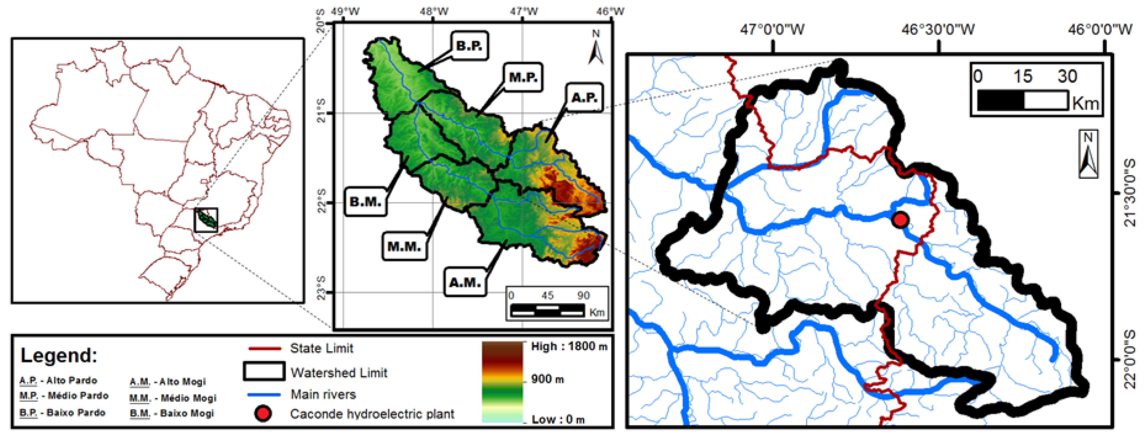
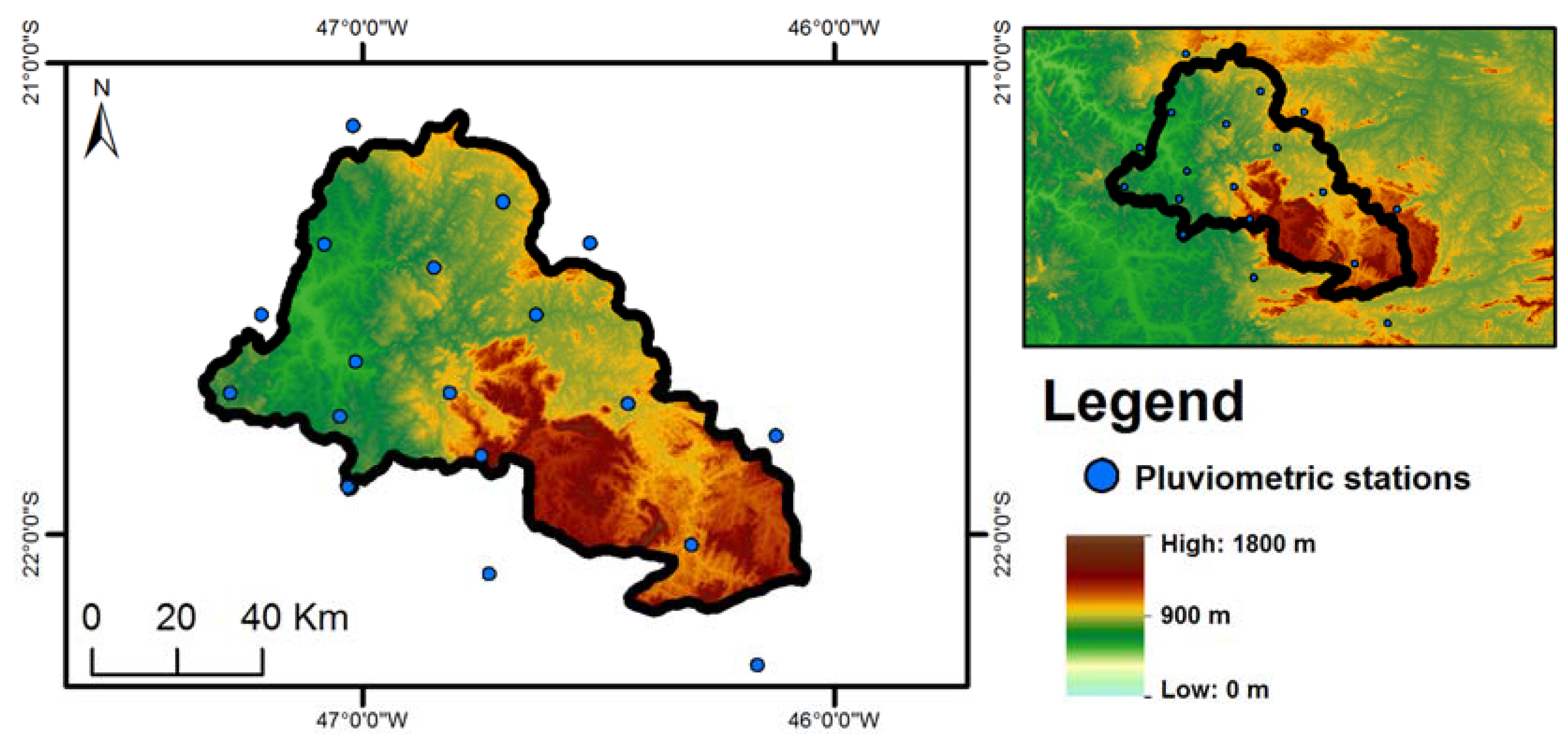
2.1. Study Area

The Alto Pardo watershed [42] is a sub-basin of the Pardo River, the main tributary of the Grande River that forms the Paraná River, in the Southeast region of Brazil, located in the northeast of the state of São Paulo and in the south-southwest of the Minas Gerais state. It is located between the parallels of 21°60′ to 22°10′ south latitude and 46°36′ to 47°20′ west longitude. The Alto Pardo watershed has a basin area of 7.182 km2 and a total of four Hydroelectric Power Plants, however the Caconde Power Plant [43] is the most important for the region, both for the total electric energy generated and for regulating the flow of the Pardo River through its reservoir. This hydroelectric plant has a drainage area of 2560 km2 and was inaugurated in the year 1966, featuring two spillways, and is the first dam of the Pardo River upstream. As seen in Figure 1, The Pardo River has two main tributaries in this sector; the Bom Jesus River downstream of the hydroelectric Caconde power plant and the Canoas River near the middle course of the river, to the west of the Alto Pardo.
The study area was chosen for this research because it is an important agricultural area at the national level, covering 27 municipalities that are partially located in the basin, and 11 of them entirely located in the basin, among them Caconde city, a touristic city which is located at the main hydroelectric plant of the whole Pardo hydrographic basin. Due to the concentration of the main sources of the Pardo River, is an important area for providing water resources for the agricultural sector of the Pardo watershed, mainly in the cultivation of coffee, sugarcane, and orange [44], which has contributed to changes in the regional landscape by agricultural activity and has demanded a large amount of water supply for irrigation.

2.2. Study Period, Data, and General Analysis

Based on the principle of this study, which seeks to investigate through the rhythmic analysis the weather types that can result in extreme rainfalls, floods, or droughts, the first step was to identify and choose a period with extreme weather conditions. Therefore, we analyzed previous studies that had identified and classified years of extreme conditions based on the standard-year method [45,46]. These surveys identified a great contrast between the years 1983 and 1984, the first one being designated as an extremely wet yet and the second classified as a dry year in the Pardo watershed. Another factor that emphasizes the choice of this period (1983–1984) was the occurrence of a very strong El Niño event in southern hemisphere in 1983 [47], which caused an extremely wet year in the South and Southeast of Brazil [48].
To support the choice of the years 1983 and 1984, a general description of the area was carried out to verify the behavior of such years from a long series of data. For this, we collected daily rainfall and natural water flow data of Caconde city, located in the center of the basin. The pluviometry station belongs to the Department of Water and Electrical Energy [49], a São Paulo state agency, and the fluviometric data were generated by the National Electric System Operator [50]. It is important to emphasize that we chose to use the natural flow data because the agency service provided model reconstructs the original water flow of the Pardo River, identifying the data that would occur if there were no human action, as the water stored in the reservoir and its use in agriculture and urban water supply [51]. This type of data has made it possible to analyze the daily flow of the river without having to take into account the expansion of the use of water resources in this stage of the research.
The general analysis of the data was made using the historical series between 1966 and 2015, a 50 year period. The choice of this time series was based on the data availability, the date of construction of the hydroelectric plant, and the occurrence of possible gaps in the daily rainfall series. In the case of gaps in the pluviometry data, we calculated the average of the daily data of the three nearest stations [52]. The bar graphs were prepared using Excel software and the boxplot graphs were generated by the statistics software R version 3.2.2..

2.3. Spatial Interpolation of Rainfall

For the mapping of the geostatistical rainfall interpolation, we use the Kriging technique [53] through the Surfer 13 software. This procedure allows for the continuity of the phenomena in space, even though gaps were left between the sampling points. The monthly rainfall data used in this study were collected through the Hidroweb tool, administered by the National Water Agency (ANA) of Brazil. In total, 18 pluviometric stations were used to perform the rainfall mapping, covering the Alto Pardo watershed and surrounding areas. Table 1 presents in detail the individual information on each of the stations.
The choice of the pluviometric stations was made through the existence of a rain gauge and the rainfall data availability for the period. The spatial coverage of the seasons can be observed in Figure 2, highlighting the 18 distribution points throughout the study area, associated with the regional orography. In the figure, it is possible to notice a good overall distribution of the rainfall stations, but it shows a lower density of stations in the southeast region of the basin, coinciding with a high altitude area and a low urbanization level, factors that contributed to the minor presence of the rain gauges. However, the existence of stations near the study area aims to compensate for, even partially, the absence of data for the interpolation process. Thus, the spatial interpolation of the rainfall monthly level during the years 1983–1984 was made seeking to provide the spatial rainfall distribution of the area, which during the qualitative analysis of the results was related to the frequency of the atmospheric systems that have passed through the region at the monthly level.

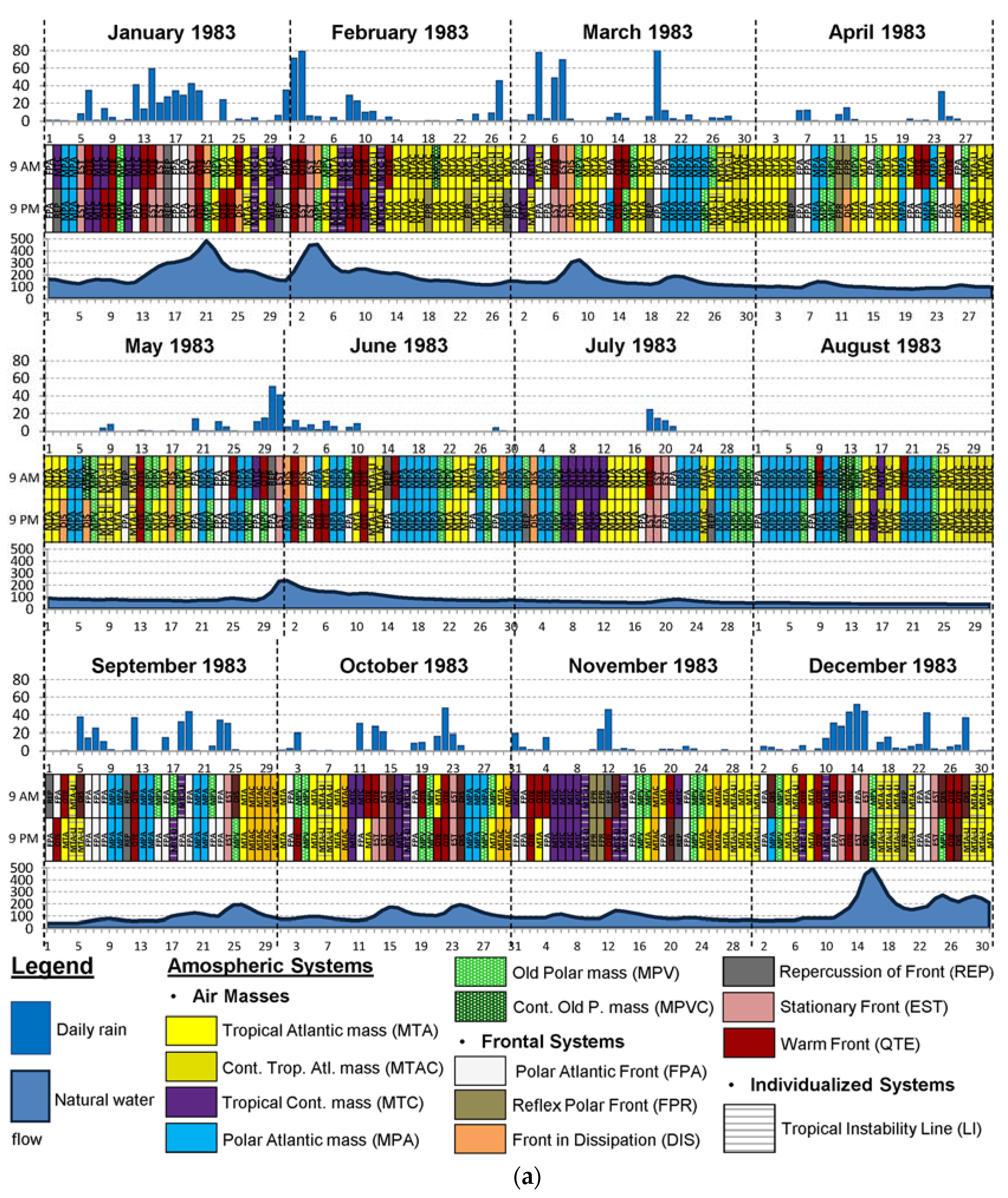
2.4. Rhythmic Analysis

To generate the rhythmic analysis, a traditional technique of Brazilian Geographic Climatology [54,55], we used weather element graphs, synoptic charts, and satellite images to understand the atmospheric circulation and weather types on a regional scale. Thus, we collected daily and hourly data of the Graminha weather station, belonging to the Department of Water and Electrical Energy [49], located at 21°34′ south latitude, 46°37′ west longitude, and at 880 m altitude in Caconde city. The data collected by the weather station refers to the following climatic elements: precipitation, air temperature, atmospheric pressure, air humidity, duration of sunshine, wind direction and intensity, and cloudiness. Satellite images were collected in daily and hourly levels through the International Satellite Cloud Climatology Project (ISCCP) of the Global ISCCP B1 Browse System (GIBBS) [56], and the synoptic charts were provided by the Brazilian Navy [57].
The rhythmic analysis was performed to identify the atmospheric circulation through the manual method, and the synoptic weather classification in daily and hourly data was applied to identify the atmospheric systems that are occurring in the period and its circulation over time. The classification of the atmospheric system was made in two daily schedules in Brazil: 9 a.m. (12 GMT) and 9 p.m. (00 GMT). It is noteworthy that a manual method, despite the criticism it received in the 21st century due to the high degree of subjectivity involved [58], brings the researcher closer to understanding the atmospheric circulation and dynamics in the region during the research, so it is still valid for use [59], even with the introduction of the automated synoptic classification and statistically sophisticated methods [60]. Regardless of the choice of method adopted in the study, all the classifications are inherently subjective to some degree [61], and these influences require the expertise of the researcher. In the case of South America, the non-existence of automated methods widely accepted for classifying “weather types” reinforces the use of the manual method in this study.
The identification of atmospheric systems in the area, at the regional level, adopted a classification system based on the relative positions of the air masses and fronts in South America [62,63], through the atmospheric flows of the anticyclones, cyclones, and frontal passages, as well as the response of climatic elements on a smaller-scale. In order to perform this procedure, we constructed the rhythmic analysis charts through the generation of line graphs of all the climatic variables collected at the Graminha weather station at the daily level, which have been aligned and organized in sequence. The graphs facilitate the analysis of variability of the data and can be observed in [41]. After that, the synoptic charts and satellite images were analyzed for each day of the year, always associating the day-to-day synoptic weather conditions with the variations of the climate data in the region, to identify the dominant atmospheric systems in the two daily schedules. This genetic classification adopted the same methodology in several other studies in Brazil [64,65,66]. The classes of the atmospheric systems and the basis of the weather types are as follows:
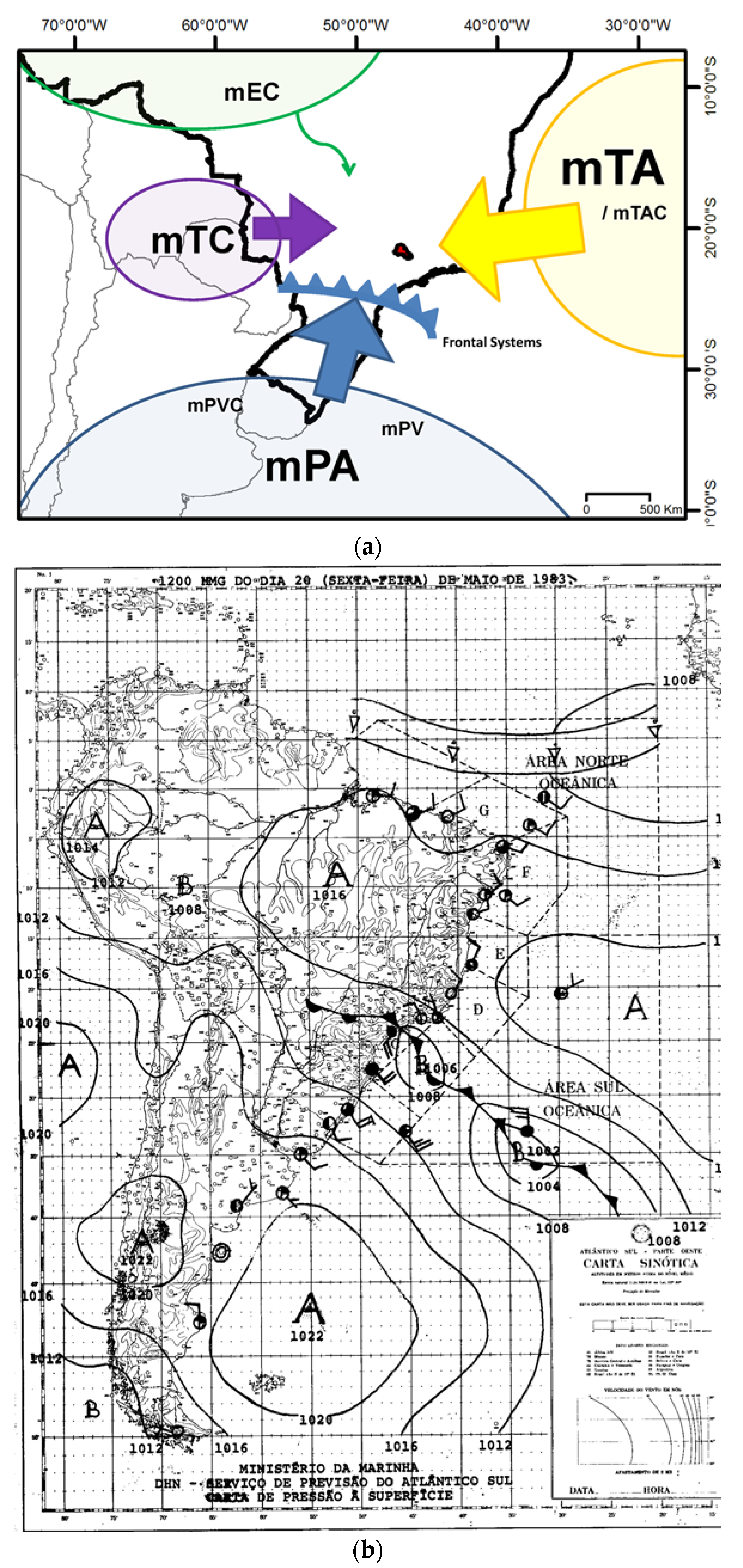
  • Air masses with tropical characteristics—Tropical Atlantic mass (mTA), Continentalized Tropical Atlantic mass (mTAC), and Tropical Continental mass (mTC); Air masses with polar characteristics—Polar Atlantic mass (mPA), Old Polar mass (mPV), and Continentalized Old Polar mass (mPVC); Air mass with equatorial characteristics—Equatorial Continental mass (mEQ).
  • Frontal Systems—Polar Atlantic Front (FPA), Reflex Polar Front (FPR), Polar Atlantic Front in Dissipation (DIS), Repercussion of Polar Atlantic Front (REP), Stationary Polar Atlantic Front (EST), Warm Front (QTE), and Occlude Polar Atlantic Front (OCL).
  • Individualized Systems—Tropical Instability Line (LI) and Atlantic Intertropical Convergence Zone (ZCIT).
The systems identified above are only those that occur frequently in southeastern Brazil. During the years 1983–1984, there were no cases of Equatorial Continental mass (mEQ), Occlude Polar Atlantic Front (OCL), and Atlantic Intertropical Convergence Zone in the Alto Pardo watershed. Regarding the origin of the systems, their synthesis [65] can be classified as follows:
  • South Currents—mPA + mPV/PVC + FPA/DIS/EST + FPR.
  • East Currents—mTA + TAC + Tropical Instability Line + QTE + REP.
  • North Current—mEQ.
  • West Current—mTC + Tropical Instability Line.
The air masses that can be observed in the southeastern region of Brazil, especially in the region of the study area, can be classified both by the tropical source region (mTA, mTAC, and mTC) and the polar source region (mPA, mPV, and mPVC). Table 2 presents a brief description of the air masses’ region of origin and explains how these atmospheric systems are classified, based on criteria to be observed and used in the synoptic charts and the variability of the climatic data for the classification of the atmospheric systems. Figure 3a illustrates the distribution of air masses by the source region, and their main incursions into the study area.
The incursion of mid-latitude polar air towards lower latitudes is linked to the cold fronts, whose trajectory and movement exhibit a different behavior throughout the year. In general, the origin of the frontal systems in the region of study is found in the advances of the mPA towards the Brazilian Southeast, generally associated with cloudy weather, high winds, and precipitation. During autumn and winter, the penetration of polar air is more intense in the Brazilian southeast, while in spring and summer, this incursion presents greater resistance by the tropical air masses [67]. The different movements of these systems are identified by the synoptic charts through their symbols, and the criteria for classification can be observed in Table 3. In addition, the table provides information on the Tropical Instability Line (LI), identified as troughs, and is associated with the air masses, not being individually classified as an atmospheric system. Figure 3b presents an example of a synoptic chart, illustrating the advance of a cold front in South America, specifically over the Alto Pardo watershed that occurred on 20 May 1983 at 9 a.m. local time (12 GMT).
After identifying all the atmospheric systems and weather types at a daily and hourly level, the next step is to analyze the data generated through a qualitative point of view. It is important to observe the frequency of the atmospheric systems over the months and seasons for the two standard-years (a wet and a dry one), and to compare them. However, the technique of rhythmic analysis consists of the analysis of the sequence of weather types, making it possible to identify the most frequent atmospheric systems, standard, or distinguished atmospheric systems in a continuous sequence. To observe the rhythm, which is more or less a regular return to the same atmospheric conditions and weather patterns, year after year, we analyzed and identify the chain of atmospheric sequences that normally occur in the region, in which the resident population is accustomed to the resulting weather types, and identified the atmospheric sequences that cause extreme episodes in the region.

3. Results

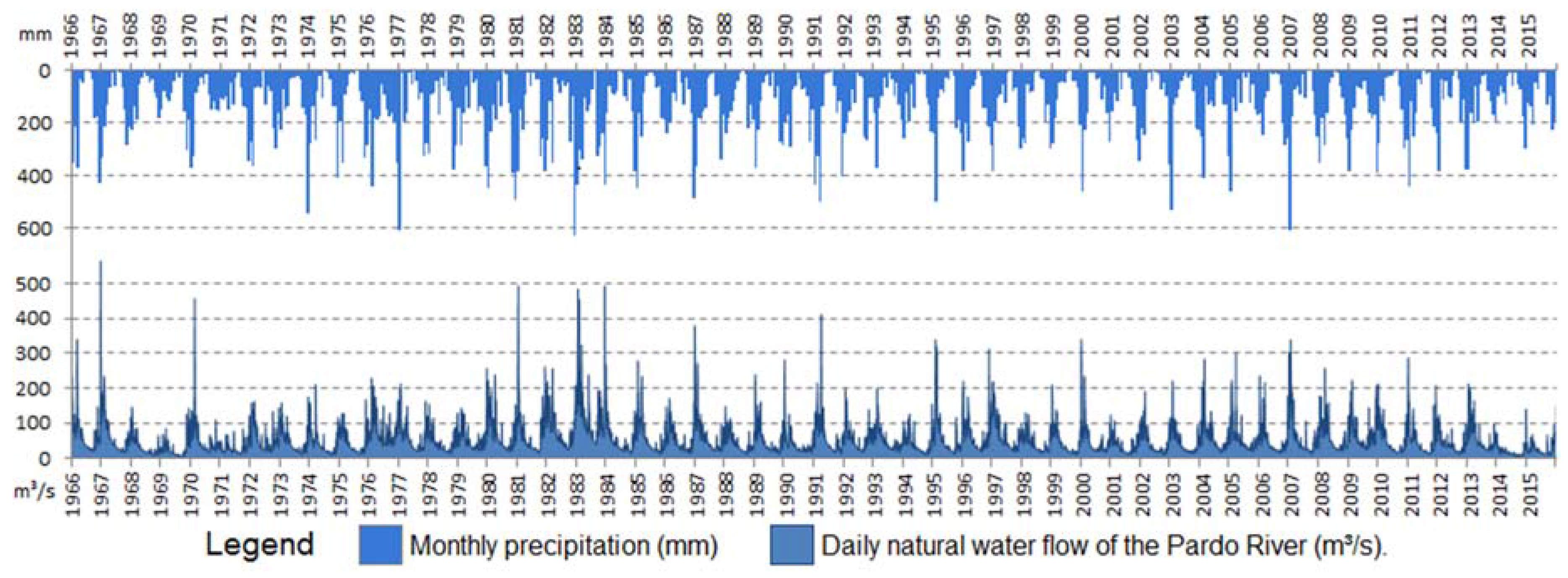
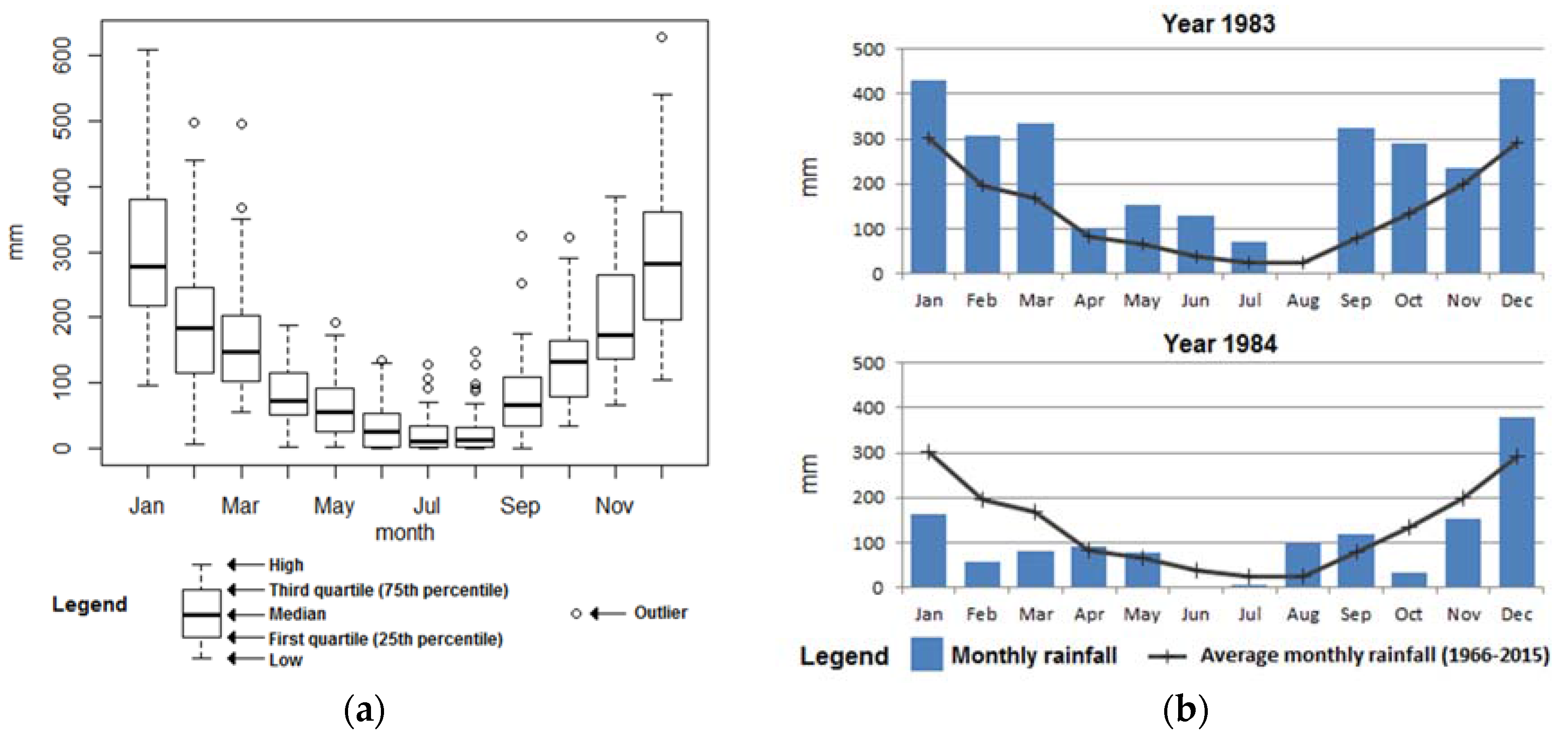
3.1. General Analysis of Rainfall Variability

The monthly variability of the rainfall volume at the Caconde station was high, as can be seen in Figure 4. A preliminary analysis of the figures enables us to decipher the measures that are present in the graph, showing the monthly volume of rain that usually occurs in the region, between the first (25th percentile) and the third quartile (75th percentile).
The seasonality of the rains observed in Figure 3a was expected, representing a regime of high precipitation in spring and summer in contrast to autumn and winter, according to the meteorological calendar of the four seasons in the southern hemisphere. However, when we observe the year 1983 in Figure 3b, only August is found to be below the historical average, and in nine months the rainfall volume was higher than the third quartile, and in some cases could be classified as an outlier, demonstrating the exceptional nature of this period. In the year 1984, seven months appear below the average, four of which are below the first quartile, but three of them (January, February, and March), are registered as dry periods in usually wet months, which gives evidence of a possible meteorological drought [68], during the months of low precipitation until the month of December. To observe the time variable of the analyzed data in this general analysis, Figure 5 relates the sequential monthly data of precipitation to the water flow in the Pardo River.
As observed in the previous figure, the seasonal rainfall variability was highlighted, evidencing the region’s rainfall regime. When associated to the natural flow of the Pardo River, there is a clear correspondence between the increase in the volume of the rainy months and the growth in the water flow, an ordinary situation observed in small and medium-sized hydrographic basins. One point of the figure that stands out is the recorded flood peaks, especially those exceeding 400 m3/s, values that are four times higher than the monthly average for the month of the greatest average flow (January—98.8 m3/s), and which can cause large impacts along the drainage of the region. In total, this number is exceeded six times in the historical series, and although the maximum peak was recorded in the last days of the year 1966, the year of 1983 presents two of these flood peaks, in the months of January and December.

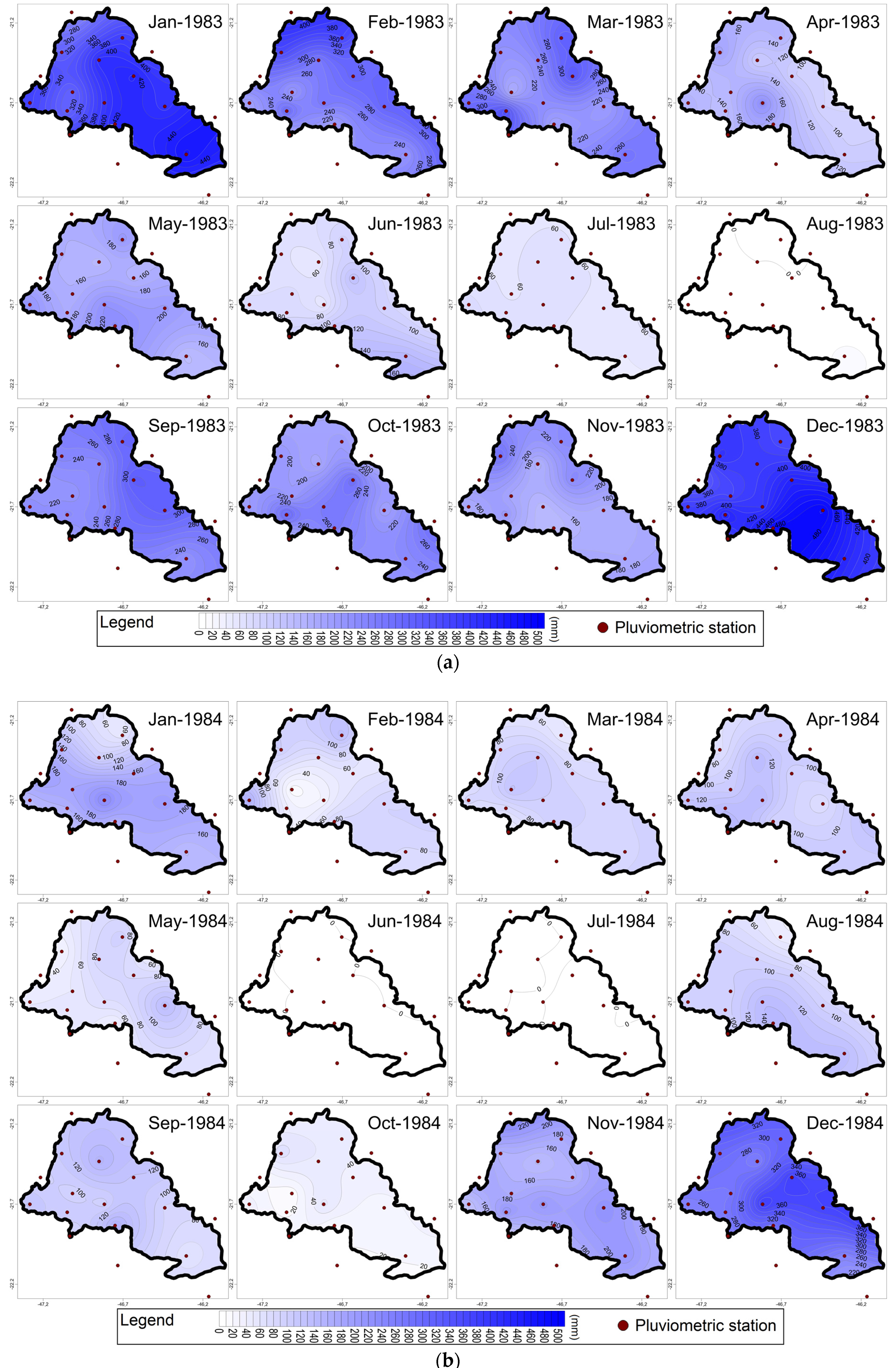
3.2. Spatial Analysis of Rainfall

In the previous procedure, the monthly precipitation volumes of the Caconde station gave an overview of the Alto Pardo basin, but described the variability from one specific rain gauge. To obtain a spatial view of the rain in the basin, Figure 6 distributes the monthly rain with contour lines, with 10 millimeters equidistant along the study area, through the kriging method for the years 1983–1984. It is important to emphasize that the precipitation maps were made to contribute to the analysis of the monthly frequency of the atmospheric systems, since they facilitate the observation of the rainfall occurrence along several pluviometric stations located in the watershed.
Even considering the spatial and temporal variability of the basin, it is possible to notice more rainfall in the high altitudes, especially in the wettest months of the period under examination. In the year 1983 it is possible to notice an extremely high volume of rainfall in the first three months, and there are cases that exceeded 400 mm monthly rainfall, and if you add up the first three months, the recorded volumes were above 1000 mm. Such volumes of rain observed contrast with the year of 1984, that presented little precipitation during the same period, such as in the case of the months of January, February, and March, which usually have more rain in the region. The normally dry months in Alto Pardo, between April and September, in the year 1983 registered a decrease in rainfall only between June and August, while in 1984 there was already a summer drought, which continued to show low precipitation by the end of November. At the end of the two years, the month of December was especially rainy for both periods.

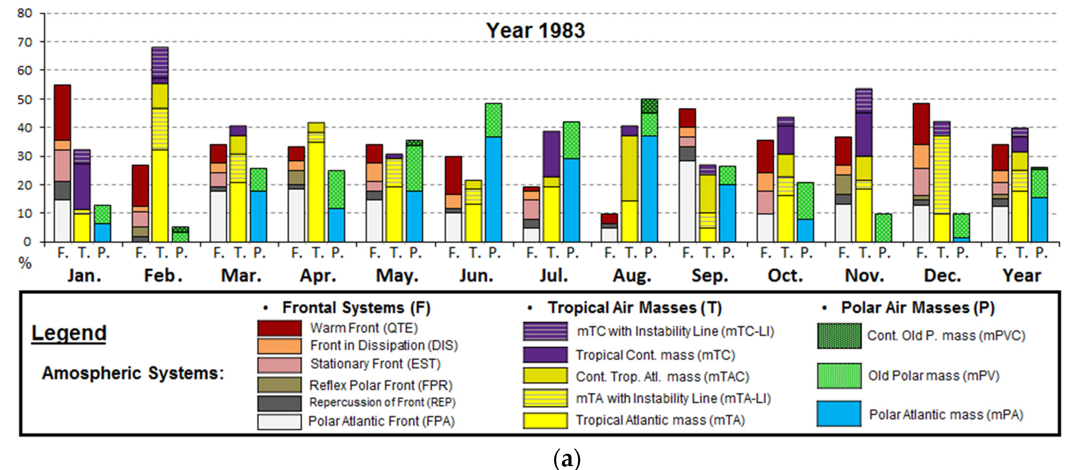
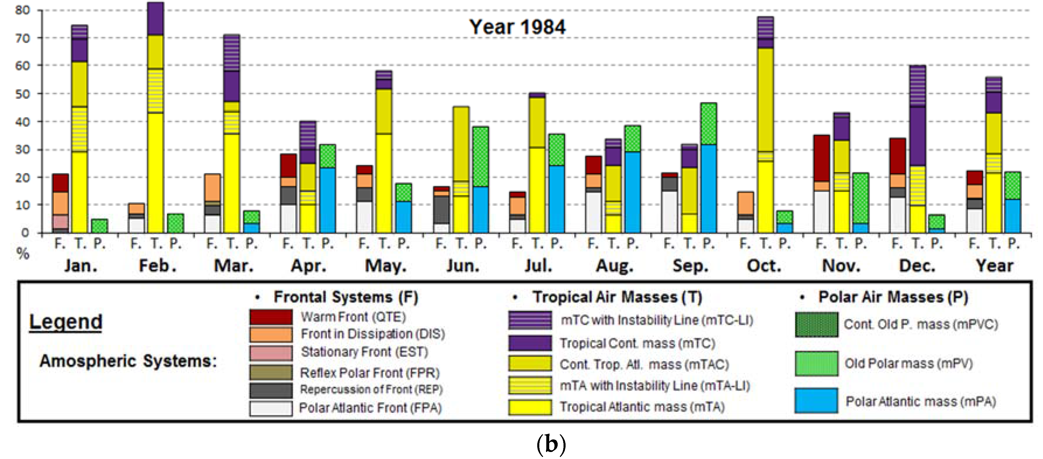
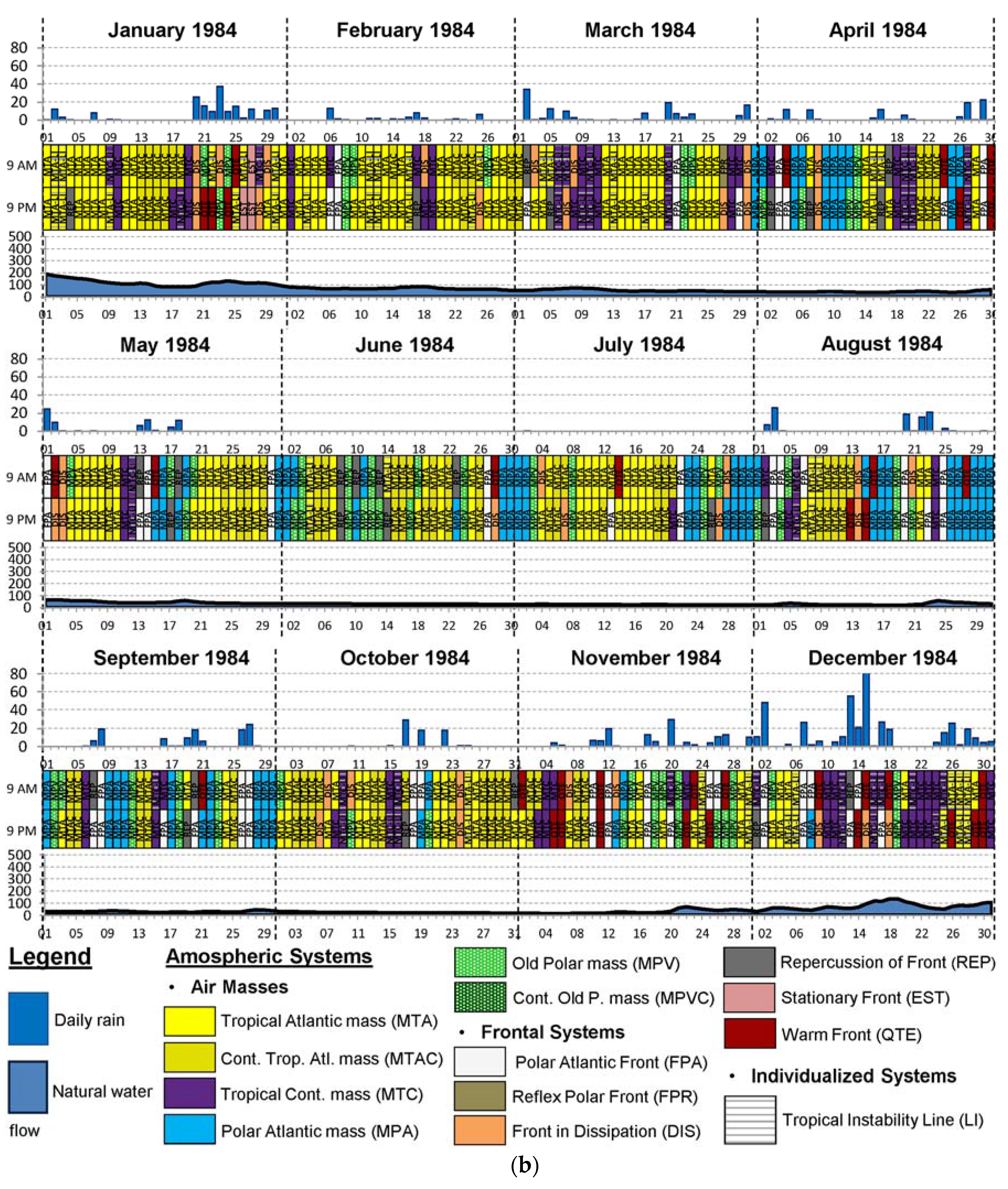
3.3. Atmospheric Systems and Rhythmic Analysis

The research procedure for the identification of atmospheric systems was applied to the years 1983 and 1984, and this stage of the study intended to synthesize the results in a clear and objective way. Table 4 and Table 5 indicate the frequency of the atmospheric systems for each of the months and the synthesis of the total frequency of the frontal systems and air masses with tropical and polar characteristics. In addition, with the aim of better summarizing the results, bar graphs were generated from the data described in the tables, which allow a better comparison between the two years. Figure 7 illustrates the frequency of the atmospheric systems at the monthly level for the year 1983 (a) and 1984 (b).
The results observed in the tables indicate a high frequency of occurrence of frontal systems and other disturbing influences in the south of Brazil in the year 1983, as compared to 1984. These results reinforce the idea that the performance of the polar front and its unfolding are the main factors that are responsible for the occurrence of intense rainfall in the state of São Paulo, as [69,70] suggests, and the observation of which will be discussed later in the paper. Another point that draws attention is the significant occurrence of the stationary front in the year 1983, while in the year 1984 it appears only in the first month of the year.
When comparing the data obtained in the monthly contribution of the atmospheric systems and rainfall maps of the previous sub-section, there is a relationship between the dry months with the predominance of air masses, both of polar or tropical origin. However, the predominance of air masses of tropical origin in the year 1984 during the first three months was numerically far superior to the year 1983, and is a fact that stands out when comparing the rain and weather types in those two years.
Nevertheless, understanding the dynamics and chaining of the atmospheric systems, and more broadly their rhythm in the daily data, is important for understanding the origin of extreme episodes and what kind of weather types are usually common in a region. Thus, we analyzed the atmospheric systems in sequence in order to understand the climatic rhythm. The systems were related to the rainfall and natural water flow at a daily level, thus giving a view of the chain of events and the repercussions on rainfall and water dynamics. Figure 8a,b shows the results of the atmospheric system associated to the described variables.
The atmospheric systems sequences observed through the rhythmic analysis chart indicate a high variability of weather types during the year 1983, especially in the rainy periods. An example of these intense atmospheric dynamics is the period from 12 to 21 of January that begins with the advance of a cold front over the region, and found resistance to the advance toward the northern region of the study area. This resistance resulted in a warm front, which stopped and remained in the region for a period of two days. On day 16, when the system threatened to move, it received more moisture from another low pressure system that remained over the Alto Pardo watershed and dissipated only on day 21. This sequence of chained frontal systems resulted in an extreme summer precipitation event, with prolonged rainfall and was largely distributed on a regional scale. As a result, the water flow reflected the heavy rains recorded along the drainage area for nine days and, on 21 January, reached the peak of 484 m3/s natural river flow. The episode described in this paragraph is just one example among several possibilities of observation through the daily analysis of the atmospheric systems.
The year 1983 recorded several rainy episodes and, in addition to that discussed in the previous paragraph, other similar episodes were recorded that were related to the stationary front, which occurred between 30 January and 5 February, 4–8 March, 28 May and 4 June, 17–21 July, 22–25 September, 11–15 and 21–24 October, and 10–15 and 22–28 December. The natural flow of the Pardo River reflected such rainy episodes, and had a rise in the data during and after each of these episodes. Among them was the day 16 December, which after the dissipation of the frontal system and the migration of the old polar mass towards the region, recorded a river flow peak of 493 m3/s.
The year 1984 was characterized by high-pressure typical conditions from the air masses, in particular the Atlantic tropical mass and mTAC, generating little rain in the study area, clear skies, and hot and dry weather types. The only period of occurrence of the stationary front recorded in the rhythmic analysis graph was the second half of January; nevertheless, the frontal system presented little intensity and did not register a very high volume of precipitation, even dominating the regional atmosphere for several days. The predominance of tropical air masses, few and low intensity frontal systems, in addition to low amounts of cold waves, was something that was significantly observed during the year through rhythmic analysis. Due to this reason, the natural water flow reduced gradually throughout the year, and did not show any peak flow, prolonging the drought and the scarcity of water resources in the region. It was only in the second half of November that it was possible to observe higher volumes of rain, brought about by the advance of frontal systems and lines of instabilities that formed the rainy month of December after a long period of drought.

4. Discussion and Conclusions

This study examined the development of the 1983–1984 atmospheric systems and analysed the rhythm between these years. Through the methodological procedures adopted, it was identified that the frontal systems were mainly responsible for the origin of the rainfall episodes at the monthly and annual levels. The combination of these highly changeable weather conditions over the course of several days resulted in 88.5% of the total volume of rainfall in 1983 that precipitated in days under the passage of frontal systems, and the hasty volume in the year 1984 during the passage of the frontal systems was 76% of the annual total. These passages of cold fronts by the incursions of the Atlantic polar mass, whether through paths of easternmost longitude and damp or through more continental and dry routes, were more frequent in the year 1983, in some cases for several sequential days, and less frequent in the year 1984, with the predominance of the air mass systems. Another point was that, due to the greater number of polar advances in the year 1983, there were more days under the dominion of the polar air masses, mainly in the winter, with a relationship between the climatic rhythm with the number of days of cold weather.
The frequency of atmospheric systems during the months, as listed in the tables, is important because it is possible to interpret the weather types that have been most frequently in the Alto Pardo region during this period. Such data, when related to the spatial distribution of rainfall, allows an interpretation of this frequency at the regional level, especially for explaining the wettest months, which increased the frequency of frontal systems that resulted in months of higher occurrence of rains upstream of the Pardo River. However, the analysis cannot be limited only to the monthly level of the frequency of atmospheric systems, because the weather types interfere at the daily level, and in some cases at the hourly level, in the natural events and human beings.
These procedures approach the climatology of the geographical analysis, by enabling the correlation of this string of weather types to the geographical variables. For example, the month of February 1983 registered high rainfall in the north of the basin, although the south of the Alto Pardo watershed has a high altitude. With the daily analysis, it is possible to check the alternating situation between the warm front and the tropical continental mass with lines of instability during the days 6 to 13, which probably contributed to the high precipitation in the northwest basin. Another fact that the monthly analysis does not show is the predominance of the tropical masses after day 14, resulting in clear skies and hot and dry weather types for almost half of the month, even in the summer of a wet year.
The frequency of frontal systems in the study area was observed mainly in the year 1983, predominating in 34.1% of days, but even in the year 1984 the fronts were frequent, more specifically in 22.4% of days. The constant currents that the South displaced to the region of the Alto Pardo watershed, and that can interfere with the weather types, occurs due to the basin being located near the Tropic of Capricorn, more specifically to the north of the line, characterized for being the threshold between the tropical and temperate zones in the southern hemisphere of the planet. In a classical climate regionalization proposed by [71] and confirmed by [72,73], it is estimated that there is a large-scale limit of the climate transition near the tropic, however this does not have an accurate and static nature [26]. That is, there is a great variability in the frequency of the frontal systems that move to the southeastern region of Brazil, and may have an impact on the source of regional rainfall.
A factor that must be considered for the planning of water resources in the region is the variation of the El Niño-Southern Oscillation (ENSO) phenomenon. Although there is no clear correlation between the rainy years and the occurrence of El Niño in Southeast Brazil, as in the southern region of Brazil [74], a very strong intensity of El Niño may have influenced the year 1983. In the analyzed region, the occurrence of the Stationary Polar Front (EST) was associated with most of the cases of intense rainfall on a timescale of two years. In addition, in some cases, this convective system is fed by moisture from the northern region of Brazil, configuring the South Atlantic Convergence Zone [75]. Its occurrence is mainly in the spring and summer, and can cause intense rainfall, and has proven to be influential for the occurrence of floods in the region.
In the case of the meteorological droughts, high-pressure atmospheric systems such as the mTA and mTAC predominated during a period normally rainy as is the case in the summer, and the chaining of these weather types, in combination with mTC and the frontal systems in dissipating toward the ocean, contributed to the low rainfall observed on the spatial scale in the first months of the year 1984, that resulted in the reduction of the levels of natural water flow throughout the year, whereas autumn and winter feature a pattern that is usually dry in the region. A similar case in southeastern Brazil is described by [76] for the summer of 2014, that proposed the existence of a blockade for the passage of frontal systems due to the anomalous high pressure over the southeast region of Brazil.
The comparison between two extreme years, a wet and a dry one, with different atmospheric circulation patterns during the year, allowed us to obtain relevant results for the study area. However, the rhythmic analysis of different weather types, and their succession over time [77], cannot be limited only to these two years of study if we aim to achieve results even more relevant and applicable. For future research, we intend to apply the method of rhythm analysis to a historical series that includes at least 15 years of data, to gradually identify the succession pattern of weather types in the Alto Pardo watershed and Southeast Brazil. The long series of data can go through qualitative analysis, and identify the chaining of the atmospheric systems at the source of rain and drought episodes, beyond the statistical treatment to try to identify the relationship between the weather type and precipitation. We hope to apply the results of the rhythmic analysis to geographical variables in the region, as in the case of floods, air quality, agriculture, health, extreme events, and several others. Finally, we want the results of the manual method of identification of the atmospheric systems to contribute in the future to build an automatic method for South America, to identify the air masses and frontal systems through the synoptic data (charts) and meteorological data.

Acknowledgments

The authors thank the Coordination of Improvement of Higher Level Personnel (CAPES) for financial support through a scholarship.

Author Contributions

This paper is the result of research conducted by Pedro Augusto Breda Fontão as part of his Master’s degree studies at the Postgraduate Program in Geography of São Paulo State University (UNESP). João Afonso Zavattini was jointly an advisor to this project and provided guidance on the analysis of the results. All authors approved the final article.

Conflicts of Interest

The authors declare no conflict of interest.

References

  1. Lima, K.C.; Satyamurty, P.; Fernández, J.P.R. Large-scale atmospheric conditions associated with heavy rainfall episodes in southeast brazil. Theor. Appl. Climatol. 2010, 101, 121–135. [Google Scholar] [CrossRef]
  2. Chi, X.; Yin, Z.; Wang, X.; Sun, Y. Spatiotemporal variations of precipitation extremes of China during the past 50 years (1960–2009). Theor. Appl. Climatol. 2015, 1–10. [Google Scholar] [CrossRef]
  3. Wollmann, C.A.; Sartori, M.G.B. Sazonalidade dos episódios de enchentes ocorridos na bacia hidrográfica do rio Caí—RS, e sua relação com a atuação do fenômeno El Niño, no período de 1982 a 2005. Rev. Bras. Climatol. 2009, 7, 103–118. [Google Scholar]
  4. Haddad, E.A.; Teixeira, E. Economic impacts of natural disasters in megacities: The case of floods in São Paulo, Brazil. Habitat Int. 2015, 45 Pt 2, 106–113. [Google Scholar] [CrossRef] [PubMed]
  5. Ebi, K.L.; Bowen, K. Extreme events as sources of health vulnerability: Drought as an example. Weather Clim. Extrem. 2016, 11, 95–102. [Google Scholar] [CrossRef]
  6. Coelho, C.A.S.; Cardoso, D.H.F.; Firpo, M.A.F. Precipitation diagnostics of an exceptionally dry event in São Paulo, Brazil. Theor. Appl. Climatol. 2016, 125, 769–784. [Google Scholar] [CrossRef]
  7. He, M.; Russo, M.; Anderson, M. Hydroclimatic Characteristics of the 2012–2015 California Drought from an Operational Perspective. Climate 2017, 5, 5. [Google Scholar] [CrossRef]
  8. Kunkel, K.E.; Pielke, R.A.; Changnon, S.A. Temporal fluctuations in weather and climate extremes that cause economic and human health impacts: A review. Bull. Am. Meteorol. Soc. 1999, 80, 1077–1098. [Google Scholar] [CrossRef]
  9. Easterling, D.R.; Evans, J.L.; Groisman, P.Y.; Karl, T.R.; Kunkel, K.E.; Ambenje, P. Observed variability and trends in extreme climate events: A brief review. Bull. Am. Meteorol. Soc. 2000, 81, 417–425. [Google Scholar] [CrossRef]
  10. Marengo, J.A.; Jones, R.; Alves, L.M.; Valverde, M.C. Future change of temperature and precipitation extremes in South America as derived from the PRECIS regional climate modeling system. Int. J. Climatol. 2009, 29, 2241–2255. [Google Scholar] [CrossRef]
  11. Intergovernmental Panel on Climate Change (IPCC). The Physical Science Basis. Contribution of Working Group to the Fifth Assessment Report of the Intergovernmental Panel on Climate Change; Cambridge University Press: New York, NY, USA, 2013. [Google Scholar]
  12. Sansigolo, C.A.; Kayano, M.T. Trends of seasonal maximum and minimum temperatures and precipitation in Southern Brazil for the 1913–2006 period. Theor. Appl. Climatol. 2010, 101, 209–216. [Google Scholar] [CrossRef]
  13. Jiang, F.; Hu, R.J.; Wang, S.P.; Zhang, Y.W.; Tong, L. Trends of precipitation extremes during 1960–2008 in Xinjiang, the Northwest China. Theor. Appl. Climatol. 2013, 111, 133–148. [Google Scholar] [CrossRef]
  14. Knapp, A.K.; Hoover, D.L.; Wilcox, K.R.; Avolio, M.L.; Koerner, S.E.; La Pierre, K.J.; Loik, M.E.; Luo, Y.; Sala, O.E.; Smith, M.D. Characterizing differences in precipitation regimes of extreme wet and dry years: Implications for climate change experiments. Glob. Chang. Biol. 2015, 21, 2624–2633. [Google Scholar] [CrossRef] [PubMed]
  15. Zandonadi, L.; Acquaotta, F.; Fratianni, S.; Zavattini, J.A. Changes in precipitation extremes in Brazil (Parana River Basin). Theor. Appl. Climatol. 2016, 123, 741–756. [Google Scholar] [CrossRef]
  16. Monteiro, C.A.F. Da necessidade de um caráter genético à classificação climática (algumas considerações metodológicas a propósito do estudo do Brasil Meridional). Rev. Geogr. 1962, 31, 29–44. [Google Scholar]
  17. Monteiro, C.A.F. A análise rítmica em climatologia: Problemas da atualidade climática em São Paulo e achegas para um programa de trabalho. Climatologia 1971, 1, 1–21. [Google Scholar]
  18. Sorre, M. Les Fondaments de la Géographie Humaine; Colin: Paris, France, 1950. [Google Scholar]
  19. Pédélaborde, P. Le Climat du Bassin Parisien: Essai d’une Méthode Rationelle de Climatologie Physique; Librairie de Medeces: Paris, France, 1957. [Google Scholar]
  20. Pédélaborde, P. Introduction a l’étude Scientifique du Clima; Centre de Documentation Cartographique: Paris, France, 1959. [Google Scholar]
  21. Pagney, P. Réflexions à propos d’ouvrages récents de Climatologie et de Météorologie. Rev. Geogr. l’Est. 1972, 12, 313–321. [Google Scholar] [CrossRef]
  22. Ribeiro, C.M. O desenvolvimento da climatologia dinâmica no Brasil. Rev. Geogr. Ens. 1982, 1, 48–59. [Google Scholar]
  23. Boin, M.N. Chuvas e Erosões no Oeste Paulista: Uma Análise Climatológica Aplicada. Ph.D. Thesis, Sao Paulo State University, Rio Claro, Brazil, 2000. [Google Scholar]
  24. Barros, J.R. A Chuva No Distrito Federal : O Regime E As Excepcionalidades Do Ritmo. Ph.D. Thesis, Sao Paulo State University, Rio Claro, Brazil, 2003. [Google Scholar]
  25. Ely, D. Teoria e Método da Climatologia Geografica Brasilera: Uma Abordagem Sobre Seus Discursos e Prácticas. Ph.D. Thesis, Sao Paulo State University, Presidente Prudente, Brazil, 2006. [Google Scholar]
  26. Zavattini, J.A. As Chuvas e as Massas de ar no Estado de Mato Grosso do Sul: Estudos Geográficos com Vista à Regionalização Climática; Cultura Acadêmica: São Paulo, Brazil, 2009; pp. 1–214. [Google Scholar]
  27. Ribeiro, A.A. Eventos Pluviais Extremos e Estiagens na Região das Missões, RS: A Percepção dos Moradores no Município de Santo Antônio das Missões. Master’s Thesis, Sao Paulo State University, Rio Claro, Brazil, 2012. [Google Scholar]
  28. Monteiro, C.A.F.; Mendonça, F.A.; Zavattini, J.A.; Sant’Anna Neto, J.L.S. The Construction of Geographical Climatology in Brazil; Alínea: Campinas, Brazil, 2015; pp. 1–170. [Google Scholar]
  29. Zavattini, J.A. Pluies Intenses et Inondations dans la Vallée du Fleuve Itajaí (Région de Santa Catarina), Brésil. Geogr. Tech. 2009, 1, 477–482. [Google Scholar]
  30. Fratianni, S.; Zavattini, J.A. Il Contributo della Climatologia Dinamica all’analisi nivometrica e risvolti turistici in Val di Susa. Mem. Della Soc. Geogr. Ital. 2009, 87, 319–332. [Google Scholar]
  31. Zavattini, J.A.; Fratianni, S. Variações do ritmo climático no piemonte italiano: Reflexos no Vale de Susa (neve e turismo) e no ‘terroir’ do barolo (produção vitivinícola). Rev. Geogr. 2016, 33, 35–63. [Google Scholar]
  32. Douguedroit, A. Quelle «exception française» en matière de «types de temps»? Norois Environ. Aménagement Soc. 2004, 33–39. [Google Scholar] [CrossRef]
  33. Baur, F. Einführung in die Großwetterkunde; Dieterich: Wiesbaden, Germany, 1948. [Google Scholar]
  34. Hess, P.; Brezowsky, H. Katalog der Grobwetterlagen Europas (1881–1976); Berichte des Deutschen Wetterdienstes in der US-Zone: Offenbach, Germany, 1952. [Google Scholar]
  35. Lamb, H.H. Types and spells of weather around the year in the British Isles: Annual trends, seasonal structure of the year, singularities. Q. J. R. Meteorol. Soc. 1950, 76, 393–429. [Google Scholar] [CrossRef]
  36. Sheridan, S.C. The redevelopment of a weather-type classification scheme for North America. Int. J. Climatol. 2002, 22, 51–68. [Google Scholar] [CrossRef]
  37. Armond, N.B. Entre Eventos e Episódios: As Excepcionalidades das Chuvas e os Alagamentos no Espaço Urbano do Rio de Janeiro. Master’s Thesis, Sao Paulo State University, Presidente Prudente, Brazil, 2014. [Google Scholar]
  38. Carrega, P. Avant-propos sur les «types de temps». Norois Environ. Aménagement Soc. 2004, 7–9. [Google Scholar] [CrossRef]
  39. Vigneau, J.-P. Un siècle de «type de temps». Epistémologie d’un concept ambigu. Norois Environ. Aménagement Soc. 2004, 11–13. [Google Scholar] [CrossRef]
  40. Nimer, E. Climatologia do Brasil, 4th ed.; Supren/Ibge: Rio de Janeiro, Brazil, 1979. [Google Scholar]
  41. Fontão, P.A.B. Ritmo das Chuvas na Bacia do Pardo (SP/MG): Reflexos na Vazão dos rios Pardo e Mogi-Guaçu. Master’s Thesis, Sao Paulo State University, Rio Claro, Brazil, 2014. [Google Scholar]
  42. Fontão, P.A.B.; Zavattini, J.A. Regionalização das chuvas anuais na Bacia do Pardo, Brasil. Cad. Prud. Geogr. 2014, Especial, 143–158. [Google Scholar]
  43. Operador Nacional do Sistema Elétrico (ONS). Plano Anual de Prevenção de Cheias Ciclo 2016/2017; Operador Nacional do Sistema Elétrico: Rio de Janeiro, Brazil, 2016; pp. 1–149. [Google Scholar]
  44. Cia Pesquisa Recursos Minerais (CPRM). Atlas Geoambiental das Bacias Hidrográficas dos Rios Mogi Guaçu e Pardo—SP: Subsídios Para o Planejamento Territorial e Gestão Ambiental; CPRM: São Paulo, Brazil, 2002; p. 77. [Google Scholar]
  45. Fontão, P.A.B.; Zavattini, J.A. As chuvas na Bacia do Pardo: Procedimentos para a escolha de ‘anos-padrão’. In XI Simpósio Brasileiro de Climatologia Geográfica, Curitiba—PR, Brazil, 2014; ABClima: Curitiba, Brazil, 2014; pp. 1989–2000. [Google Scholar]
  46. Zandonadi, L. As Chuvas na Bacia do Paraná: Aspectos Temporais, Espaciais e Rítmicos. Master’s Thesis, Sao Paulo State University, Rio Claro, Brazil, 2009. [Google Scholar]
  47. National Weather Service. El Niño—Southern Oscillation (ENSO). Available online: http://www.cpc.ncep.noaa.gov/products/precip/CWlink/MJO/enso.shtml (accessed on 2 February 2017).
  48. Grimm, A.M.; Aceituno, P. El niño, novamente! Rev. Bras. Meteorol. 2015, 30, 351–357. [Google Scholar] [CrossRef]
  49. DAEE. Banco de Dados Hidrológicos. Available online: http://www.hidrologia.daee.sp.gov.br/ (accessed on 10 October 2016).
  50. Operador Nacional do Sistema Elétrico (ONS). Séries de Vazão. Available online: http://www.ons.org.br/operacao/vazoes_naturais.aspx (accessed on 10 October 2016).
  51. Operador Nacional do Sistema Elétrico (ONS). Atualização De Séries Históricas De Vazões—Período 1931 a 2015; Operador Nacional do Sistema Elétrico: Rio de Janeiro, Brazil, 2016. [Google Scholar]
  52. Tucci, C.E.M. Hidrologia: Ciência e Aplicação, 4th ed.; ABRH-EPUSP: Porto Alegre, Brazil, 2013. [Google Scholar]
  53. Tabios, G.Q.; Salas, J.D. A comparative analysis of techniques for spatial interpolation of precipitation. J. Am. Water Resour. Assoc. 1985, 21, 365–380. [Google Scholar] [CrossRef]
  54. Zavattini, J.A. Estudos do Clima No Brasil; Alínea: Campinas, Brazil, 2004. [Google Scholar]
  55. Neves, G.; Gallardo, N.; Vecchia, F. A Short Critical History on the Development of Meteorology and Climatology. Climate 2017, 5, 23. [Google Scholar] [CrossRef]
  56. Knapp, K.R. Scientific data stewardship of International Satellite Cloud Climatology Project B1 global geostationary observations. J. Appl. Remote Sens. 2008, 2, 023548. [Google Scholar] [CrossRef]
  57. Marinha do Brasil. Centro de Hidrografia da Marinha. Available online: http://www.mar.mil.br/dhn/chm/meteo/prev/cartas/cartas (accessed on 15 October 2016).
  58. Huth, R.; Beck, C.; Philipp, A.; Demuzere, M.; Ustrnul, Z.; Cahynová, M.; Kyselý, J.; Tveito, O.E. Classifications of atmospheric circulation patterns: Recent advances and applications. Ann. N. Y. Acad. Sci. 2008, 1146, 105–152. [Google Scholar] [CrossRef] [PubMed]
  59. Yarnal, B.; Comrie, A.C.; Frakes, B.; Brown, D.P. Developments and prospects in synoptic climatology. Int. J. Climatol. 2001, 21, 1923–1950. [Google Scholar] [CrossRef]
  60. Lewis, A.B.; Keim, B.D. History and Applications of Manual Synoptic Classification. Ref. Mod. Earth Syst. Environ. Sci. 2015, 1–7. [Google Scholar] [CrossRef]
  61. Lee, C.C.; Sheridan, S.C. Synoptic Climatology: An Overview. Ref. Mod. Earth Syst. Environ. Sci. 2015, 1–7. [Google Scholar] [CrossRef]
  62. Serra, A.; Ratisbona, L. As Massas de ar da América do Sul; Ministério da Agricultura, Serviço de Meteorologia: Rio de Janeiro, Brazil, 1942.
  63. Monteiro, C.A.F. Sobre Um Índice de Participação das Massas de Ar e suas Possibilidades de Aplicação à Classificação Climática. Rev. Geogr. 1964, 33, 59–69. [Google Scholar]
  64. Mendonça, F. La connaissance du climat au brésil: Entre le vernaculaire et le scientifique. Confin. Rev. Fr. Brésilienne Géogr. Rev. Fr. Bras. Geogr. 2012. [Google Scholar] [CrossRef]
  65. Zavattini, J.A.; Boin, M.N. Climatologia Geográfica: Teoria e Prática de Pesquisa; Alínea: Campinas, Brazil, 2013. [Google Scholar]
  66. Ogashawara, I.; Zavattini, J.A.; Tundisi, J.G. The climatic rhythm and blooms of cyanobacteria in a tropical reservoir in São Paulo, Brazil. Braz. J. Biol. 2014, 74, 72–78. [Google Scholar] [CrossRef] [PubMed]
  67. Mendonça, F.; Danni-Oliveira, I.M. Climatologia: Noções Básicas e Climas do Brasil; Oficina de Textos: São Paulo, Brazil, 2007. [Google Scholar]
  68. Wilhite, D.A. Drought as a natural hazard: concepts and definitions. In Drought: A Global Assessment; Routledge: London, UK, 2000; pp. 3–18. [Google Scholar]
  69. Monteiro, C.A.F. A Frente Polar Atlântica e as Chuvas de Inverno na Fachada Sul-Oriental do Brasil (Contribuição Metodológica à Análise Rítmica dos Tipos de Tempo no Brasil); USP/IG: São Paulo, Brazil, 1969. [Google Scholar]
  70. Tarifa, J.R. Fluxos Polares e as Chuvas de Primavera-Verão no Estado de São Paulo; Doctoral Dregree-USP: São Paulo, Brazil, 1975. [Google Scholar]
  71. Strahler, A.H. Physical Geography; John Wiley & Sons: New York, NY, USA, 1951. [Google Scholar]
  72. Monteiro, C.A.F. A Dinâmica Climática e as Chuvas no Estado de São Paulo: Estudo Geográfico sob a Forma de Atlas; USP/Igeog: São Paulo, Brazil, 1973. [Google Scholar]
  73. Monteiro, C.A.F. A Dinâmica Climática e as Chuvas no Estado de São Paulo; UNESP/Ageteo: Rio Claro, Brazil, 2000. [Google Scholar]
  74. Nery, J.T. Dinâmica climática da região sul do Brasil. Rev. Bras. Climatol. 2005, 1, 61–75. [Google Scholar]
  75. Carvalho, L.M.V.; Jones, C.; Liebmann, B. The South Atlantic Convergence Zone: Persistence, intensity, form, extreme precipitation and relationships with intraseasonal activity. J. Clim. 2004, 17, 88–108. [Google Scholar] [CrossRef]
  76. Coelho, C.A.; de Oliveira, C.P.; Ambrizzi, T.; Reboita, M.S.; Carpenedo, C.B.; Campos, J.L.P.S.; Tomaziello, A.C.N.; Pampuch, L.A.; de Souza Custódio, M.; Dutra, L.M.M. The 2014 southeast Brazil austral summer drought: Regional scale mechanisms and teleconnections. Clim. Dyn. 2016, 46, 3737–3752. [Google Scholar] [CrossRef]
  77. Monteiro, C.A.F. Clima e Excepcionalismo: Conjecturas Sobre o Desempenho da Atmosfera Como Fenômeno Geográfico; UFSC: Florianópolis, Brazil, 1991. [Google Scholar]
Figure 1. The Alto Pardo watershed.
Climate 05 00047 g001
Figure 2. Elevation and pluviometry stations in the Alto Pardo watershed.
Climate 05 00047 g002
Figure 3. (a) Air masses by the source region and their main incursions into the Alto Pardo according to the data of [28,67] (b) Example of a synoptic chart provided by [57] (20 May 1983).
Climate 05 00047 g003
Figure 4. (a) 50-year monthly rainfall (1966–2015) with boxplot comparison; (b) 1983 and 1984 monthly rainfall.
Climate 05 00047 g004
Figure 5. 50-year rainfall and natural water flow series (1966–2015) in the Caconde station.
Climate 05 00047 g005
Figure 6. Distribution of monthly rainfall in the Alto Pardo watershed in the year (a) 1983; (b) 1984.
Climate 05 00047 g006
Figure 7. Atmospheric systems frequency at the monthly level in the tear (a) 1983; (b) 1984.
Climate 05 00047 g007aClimate 05 00047 g007b
Figure 8. Rhythm of the atmospheric systems associated with rainfall and natural water flow in the year (a) 1983; (b) 1984.
Climate 05 00047 g008aClimate 05 00047 g008b
Table 1. List of the 18 pluviometric stations used in the spatial interpolation.
Pluviometric Station 1Latitude (S)Longitude (W)Elevation (m)
1Fazenda Carvalhais−21.13−47.02873
2Guaxupé−21.29−46.70828
3Muzambinho−21.38−46.521040
4Sítio Esplanada−21.38−47.08660
5Fazenda Açude−21.43−46.85840
6Fazenda Morrinhos−21.53−47.22610
7Caconde−21.53−46.63880
8Usina Limoeiro−21.63−47.02580
9Tambau−21.70−47.28730
10São Sebastião da Grama−21.70−46.82920
11Cachoeira do Carmo−21.72−46.44875
12Casa Branca−21.75−47.05670
13Cacheira Poço Fundo−21.79−46.12820
14São Roque da Fartura−21.83−46.751310
15Lagoa Branca−21.90−47.03700
16Beira de Santa Rita−22.02−46.301140
17Fazenda Paraíso−22.08−46.73810
18Borda da Mata−22.28−46.16854
1 Source: National Water Agency.
Table 2. Air masses: origin and criteria for classification.
TypeOriginCriteria for Classification 1
mTASouth Atlantic Anticyclone high-pressure system over tropical latitudes, presenting high temperature and humidity characteristics.The presence of isobars of the high pressure sector influencing the study area, through the air flows of east and northeast observed in the synoptic chart, reinforced by the tropical characteristics of the climatic variables, such as high temperatures and relative humidity.
mTACThis system is formed from the mTA, when it remains over the continent for a few days and although it still has a high pressure, it loses its original properties, mainly decreasing the relative humidity.Always preceded by mTA and presenting a pressure pattern similar to this air mass, it is distinguished by the significant change in the climatic variables that can be observed in the data of the study area, such as the great decrease in relative humidity, higher maximum temperature, clear sky, and high insolation.
mTCLow pressure system of Chaco, in the Tropic region east of the Andes, with cyclonic circulation of the surface and anticyclonic at the upper levels, as a consequence of the intermittent thermal-orographic depression. The characteristics of this air mass is hot and dry.The presence of isobars of the low pressure sector of the center of South America in the study area, coming from the air flows to the west observed in the synoptic chart. A large decrease in relative humidity, elevation of maximum temperature, clear sky, and high insolation are characteristics of this air mass.
mPAAnticyclone with the source region in the Atlantic Ocean in southern South America, presenting cold temperatures as the main characteristic. Because of the high pressure, this air mass tends to flow towards the lower latitudes.It always occurs after the passage of a cold front, when the incursion of this anticyclonic system happens. In addition to observing the high pressure influencing the region in the synoptic charts, another factor that should be noted is the weather data, mainly the presence of lower temperatures and high atmospheric pressure for the area.
mPVThis system is formed from the mPA, when it remains outside the source region for a few days and loses its original properties, mainly raising its temperature.In the synoptic chart one must observe the incursion and the influence of the polar anticyclone on the study area. However, it differs clearly from mPA by the sensible decrease of the original atmospheric pressure, in addition to the higher temperature when acquiring the tropical characteristics.
mPVCSimilar to mPV, this system is formed from mPA when it loses its original properties; however, it was modified by the continental trajectory of the anticyclone migration, mainly decreasing the relative humidity.It presents the same criteria of mPV, however it is classified as mPVC when the anticyclone trajectory occurs inside the continent, resulting in very low relative humidity.
1 Source: Table generated according to data provided by [62,65,67].
Table 3. Frontal Systems and Individualized Systems: criteria for classification.
TypeCriteria for Classification 1
FPAThe system is represented in the synoptic chart as the limits of mPA’s advance toward the study area. A drop in temperature and atmospheric pressure should be noted in the climatic variables, in addition to an increase in the relative humidity and cloudiness.
FPRThis system occurs when, after the polar air has advanced over the region of study, a trough is observed in this anticyclone forming a squall line, which can be identified in the synoptic chart by the symbol of frontolysis in the continent and the symbol of frontogenesis in the ocean. Increased humidity and cloudiness can be observed in the climate data.
DISIt is represented in the synoptic chart as a frontolysis over the study area. In the climatic variables, an increase of the sunshine and decrease of the humidity and cloudiness can be observed during the day.
REPThis system is classified when an approximation of the FPA is observed through the synoptic chart, but it does not occur directly over the study area. Even so, a significant change has already been observed in the climatic variables such as increased cloudiness and humidity, decreased thermal amplitude and, in most cases, precipitation.
ESTThis system has a specific symbol for stationary front in the synoptic chart, and can be classified when a frontal system is moving very slowly or is stalled for a few days. Mostly cloudiness and precipitation are observed.
QTEThis system can be identified as a warm front in the synoptic chart. It is usually associated with increased cloudiness and temperature, and the occurrence of precipitation.
LILines of instability may appear on air masses, especially mTA and mTC, identified in the synoptic chart as a trough line. These lines of pressure intensify the convective movement. Rainfall and increase of the humidity can usually be observed.
1 Source: Table generated according to data provided by [62,65,67].
Table 4. Atmospheric systems frequency at the monthly level in the year 1983.
Atmospheric System (%)Months—1983Year
Jan.Feb.Mar.Apr.MayJun.Jul.Aug.Sep.Oct.Nov.Dec.
FPA14.50.017.718.314.510.04.84.828.39.713.312.912.5
REP6.51.81.61.73.21.73.21.65.00.03.31.62.6
FPR0.03.60.05.00.00.00.00.00.00.06.71.61.4
EST11.35.44.80.03.20.06.50.03.38.10.09.74.4
DIS3.21.83.23.36.55.03.20.03.36.53.38.14.0
QTE19.414.36.55.06.513.31.63.26.711.310.014.59.3
MTA9.732.121.035.019.413.319.414.55.016.118.39.717.7
MTA-LI1.614.39.73.39.75.00.00.05.06.53.327.47.1
MTAC0.08.96.53.30.03.33.222.613.38.18.30.06.4
MTC16.11.83.20.01.60.016.13.20.09.715.00.05.6
MTC-LI4.810.70.00.00.00.00.00.03.33.28.34.82.9
MPA6.50.017.711.717.736.729.037.120.08.10.01.615.6
MPV6.53.68.113.316.111.712.98.16.712.910.08.19.9
MPVC0.01.80.00.01.60.00.04.80.00.00.00.00.7
Frontal Systems54.826.833.933.333.930.019.49.746.735.536.748.434.1
Tropical Masses32.367.940.341.730.621.738.740.326.743.553.341.939.7
Polar Masses12.95.425.825.035.548.341.950.026.721.010.09.726.2
Table 5. Atmospheric systems frequency at the monthly level in the year 1984.
Atmospheric System (%)Months—1984Year
Jan.Feb.Mar.Apr.MayJun.Jul.Aug.Sep.Oct.Nov.Dec.
FPA0.05.26.510.011.33.34.814.515.04.815.012.98.6
REP1.61.73.26.74.810.01.61.65.01.60.03.23.4
FPR0.00.01.60.00.00.00.00.00.00.00.00.00.1
EST4.80.00.00.00.00.00.00.00.00.00.00.00.4
DIS8.13.49.73.34.81.76.54.80.08.13.34.84.9
QTE6.50.00.08.33.21.71.66.51.70.016.712.94.9
MTA29.043.135.510.035.513.330.66.56.725.815.09.721.7
MTA-LI16.115.58.15.00.05.00.04.80.03.26.714.56.6
MTAC16.112.13.210.016.126.717.712.916.737.111.70.015.0
MTC8.112.111.35.03.20.01.66.56.73.28.321.07.2
MTC-LI4.80.012.910.03.20.00.03.21.78.11.714.55.1
MPA0.00.03.223.311.316.724.229.031.73.23.31.612.3
MPV4.86.94.88.36.521.711.39.715.04.818.34.89.7
MPVC0.00.00.00.00.00.00.00.00.00.00.00.00.0
Frontal Systems21.010.321.028.324.216.714.527.421.714.535.033.922.4
Tropical Masses74.282.871.040.058.145.050.033.931.777.443.359.755.6
Polar Masses4.86.98.131.717.738.335.538.746.78.121.76.522.0

