Review

Hydrological Climate Change Impact Assessment at Small and Large Scales: Key Messages from Recent Progress in Sweden

1
Research & Development (hydrology), Swedish Meteorological and Hydrological Institute, 601 76 Norrköping, Sweden
2
Department of Civil, Environmental, and Natural Resources Engineering, Luleå University of Technology, 97187 Luleå, Sweden
3
Rossby Centre, Swedish Meteorological and Hydrological Institute, 601 76 Norrköping, Sweden
4
Department of Water Resources Engineering, Lund University, Box 118, 221 00 Lund, Sweden
*
Author to whom correspondence should be addressed.
Climate 2016, 4(3), 39; https://doi.org/10.3390/cli4030039
Submission received: 1 April 2016 / Revised: 29 July 2016 / Accepted: 29 July 2016 / Published: 24 August 2016
(This article belongs to the Special Issue Impact of Climate Change on Water Resources)

Abstract

:
Hydrological climate change impact assessment is generally performed by following a sequence of steps from global and regional climate modelling, through data tailoring (bias-adjustment and downscaling) and hydrological modelling, to analysis and impact assessment. This “climate-hydrology-assessment chain” has been developed with a primary focus on applicability to a medium-sized rural basin, which has been and still is the main type of domain investigated in this context. However, impact assessment is to an increasing degree being performed at scales smaller or larger than the medium-sized rural basin. Small-scale assessment includes e.g., impacts on solute transport and urban hydrology and large-scale assessment includes e.g., climate teleconnections and continental modelling. In both cases, additional complexity is introduced in the process and additional demands are placed on all components involved, i.e., climate and hydrology models, tailoring methods, assessment principles, and tools. In this paper we provide an overview of recent progress with respect to small- and large-scale hydrological climate change impact assessment. In addition, we wish to highlight some key issues that emerged as a consequence of the scale and that need further attention from now on. While we mainly use examples from work performed in Europe for illustration, the progress generally reflects the overall state of the art and the issues considered are of a generic character.

1. Introduction

Climate, as manifested in long-term patterns of day-to-day weather, is the main driver of hydrological processes and therefore climate change (CC) will also affect hydrology and water resources. Global warming is expected to affect the hydrological cycle in different ways. Some of the expected hydrological change is attributed to precipitation changes, e.g., regional redistribution caused by modified tracks of cyclones and storms as well as higher extreme intensities in a warmer atmosphere (e.g., [1,2]). Actual evapotranspiration may change not only because of warming but also because of changes in e.g., surface soil moisture, the length of the vegetation period, wind characteristics, atmospheric humidity, and net radiation. Also, the temperature itself may directly affect the hydrological regime, especially in basins where snow accumulation and melt is significant (e.g., [3,4,5]).
Because of the substantial expected impact of global warming on hydrology, much effort has been spent over the last two decades assessing future hydro-climatology. Water is involved in all societal sectors and there is great concern over how future changes will affect business, safety, and ecosystem sustainability. Climate adaptation measures are being pushed by many policy makers in the water sector. Key research activities include analysing historical trends in runoff and discharge (e.g., exploring relationships between hydrology and large-scale climate through teleconnections) and making projections of future hydrological states. The latter is typically carried out in a top-down approach where climate model output data, usually precipitation and temperature from a Regional Climate Model (RCM), are extracted for the basin in question and then used to drive a hydrological model. It was early recognized that uncertainties in climate modelling had a strong influence on hydrological impact assessments (e.g., [3]). Methods for bias-adjustment and downscaling (in the following, jointly termed tailoring of climate model data) were developed and these efforts have gradually expanded into a research field of their own; currently a large variety of approaches and techniques is available (e.g., [6,7,8,9,10,11]).
Most hydrological CC impact modelling has focused on medium-sized (on the order of 1000 km2) and predominantly rural basins. Hydrological models are generally set up for single river basins, often divided into sub-basins, and already existing setups are normally used in CC impact studies. The typical scale and character of the basins imply that the typical RCM time step (one day) and spatial resolution (25–50 km) are sufficient for resolving the relevant spatio-temporal variability in meteorological forcing, even if bias needs to be handled. Although many other approaches have been made, there is today a rather standardized procedure for hydrological CC impact assessment in this context, including the following steps: 1) RCM downscaling of Atmospheric-Ocean General Circulation Model (AOGCM) output over a regional domain, 2) extraction of RCM output on basin scale, 3) RCM data tailoring, 4) hydrological simulations, and 5) analysis and presentation of future changes. This type of assessment is today commonly performed operationally by consultants, in parallel with ongoing research on different aspects of this procedure.
There is, however, a need to consider hydrological impacts in other cases besides the medium-sized rural basin. On the one hand, there is the very local scale associated with e.g., single fields or urban blocks. In this case, hydrological (and hydraulic) processes are governed by the local climate with a very pronounced temporal variability, requiring model resolutions far beyond the typical RCM resolution. This is particularly crucial in the case of precipitation, considering its extreme small-scale variability (e.g., [12]). On the other hand, very large-scale (e.g., continental), multi-basin hydrological model systems are developed and applied to an increasing degree, e.g., to provide an international overview of climate effects on water resources and hydrological extremes or as input to oceanographic models. These large domains may contain largely varying climatic regimes, which places high demands on hydrological modelling in ungauged basins, historical reference data, climate models, and bias-adjustment methods.
This paper presents a synthesis of recent (~5 years) CC impact research in Sweden for small and large scales, with development and application of all the above components, i.e., climate models, bias-adjustment and downscaling, and hydrological or hydraulic modelling. The small-scale studies were mainly focused on impacts on water quality at field and urban scale. The large-scale studies investigated future changes in discharge, as well as other hydrological variables and nutrients at the national and continental scale. The aim of this paper is to share some experiences gained in this work and in particular some main messages obtained from the results, to highlight specific issues—challenges, limitations, and pitfalls—associated with the progress in small- and large-scale hydrological CC impact assessment. These issues are not new; they have been noticed and discussed previously, albeit to various degrees, but we are not aware of any publication with a dedicated overview in a synthesis paper. Furthermore, other relevant issues certainly exist in this context but we limit ourselves to the major concerns and case studies within our recent experience. Each issue highlighted in this paper is linked to progress for impact assessment at the small or the large scale, which is illustrated, explained, and discussed by making reference to experience gained and results published elsewhere. Before presenting the progress, a brief discussion of the state of the art with respect to hydrological CC impact assessment is included as a baseline. It should be emphasized that although we use results from our specific methods and models (AOGCM/RCM, bias-adjustment and downscaling, hydrological modelling, etc.) in our specific domains for illustration (Sweden and Europe as a whole), the intention is to represent the overall current state of the research field.

2. Hydrological Impacts of Climate Change: State of the Art

In this section we outline the three main steps in the “climate-hydrology-assessment chain” commonly used in hydrological CC impact assessment (Figure 1):
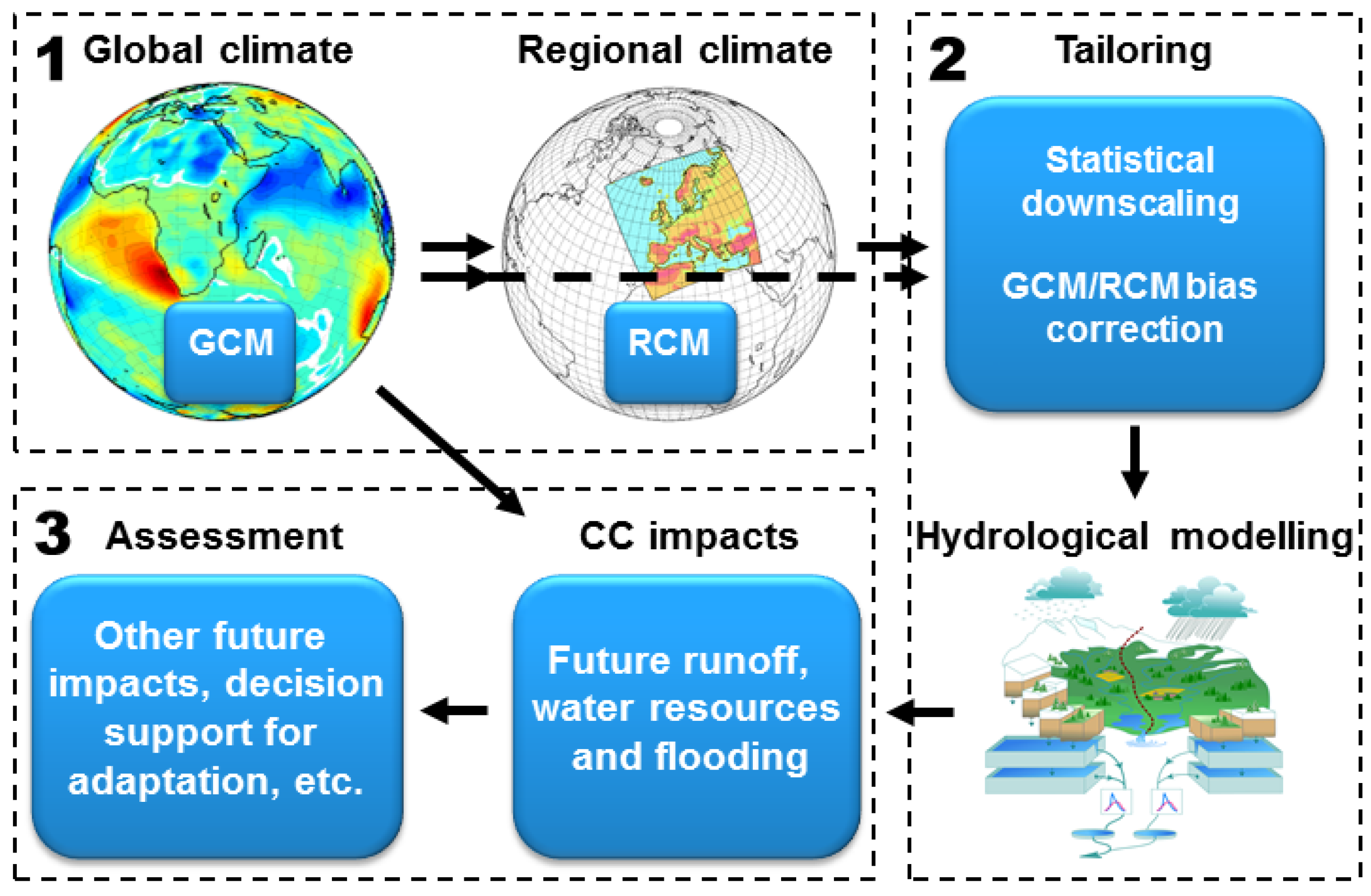
  • Climate modelling. AOGCMs are used to make future climate projections, which are commonly dynamically downscaled by RCMs.
  • Tailoring and hydrological modelling. Simulations with hydrological models, commonly preceded by tailoring of the GCM or RCM output. This tailoring may include bias-adjustment and/or downscaling.
  • Impact assessment. The results are post-processed in statistical analysis, to be useful as decision support to various societal sectors. They are also analysed to attribute hydrological processes and assess the importance of CC in relation to other changes, in order to optimize adaptation measures.
The description below aims at being generally applicable but with some specific examples of activities, models, and tools that constitute the baseline for the particular work presented here.

2.1. Climate Modelling

Information about possible future CC under global warming is becoming an integral part of developing suitable adaptation strategies at global, national, regional, and local levels. The primary source of such information is state-of-the-art AOGCMs that simulate possible CC under a range of future greenhouse gas emission or concentration scenarios. Over last few years 20 modelling groups using more than 50 models have participated in the Coupled Model Intercomparison Project phase 5 (CMIP5), generating a large multi-model ensemble of CC simulations [13]. Although the complexity and resolution of AOGCMs are both increasing, computational demands still limit the use of high-resolution AOGCMs for generating large ensembles of long multi-century climate simulations. A typical grid spacing in CMIP5 is in the range 100–250 km, which is not sufficient to provide CC information on the regional to local scale required by many users. Besides long-term projections, typically until the end of this century, AOGCMs are increasingly being used for predictions on more near-future, decadal time scales [14,15].
A common approach is to supplement global models by empirical-statistical or dynamical downscaling (ESD or DD respectively). To derive regional climate information, ESD applies a statistical relationship between information from AOGCMs and local-scale processes, while DD uses RCMs driven by AOGCMs. Over the past decade many international projects have applied RCMs to generate high-resolution, multi-model ensembles driven by AOGCMs (e.g., [16,17,18,19]). All regional downscaling projects have made significant contributions to understanding of regional CC but there have been different experiment designs, archiving protocols, standards, etc., and therefore limited transfer of knowledge between different regions. The Coordinated Regional Climate Downscaling Experiment (CORDEX) [20,21], established in 2009 and sponsored by the World Climate Research Programme (WCRP), aims to fill such gaps by coordinating international efforts in regional climate downscaling introducing predefined grids, experiment protocols, output formats, and variables. One of the main aims of CORDEX is to make regional climate simulations easily and openly available for end-user communities at regional and local levels.
In order to allow wide participation in the CORDEX activities it was decided to make the base CORDEX resolution about 50 km. It was also recommended that all RCM groups first run their RCMs at the 50 km resolution and then, if resources were available, at a higher resolution to explore the benefits of increased RCM resolution. In Europe two large international downscaling projects have already been finished: 10 RCM groups have run their simulations at 50 km resolution in PRUDENCE and 16 RCM groups at higher 25 km resolution in ENSEMBLES. Based on these previous achievements at 50 and 25 km resolution, in Euro-CORDEX—a European branch of the CORDEX project with 29 participating groups (http://www.euro-cordex.net/)—the base resolution has been set to 12 km. Most of the planned Euro-CORDEX simulations have been completed and a number of articles providing the first Euro-CORDEX results have been published [22,23,24,25]. Part of the completed Euro-CORDEX simulations has already been made openly available on the Earth System Grid Federation (ESGF)—an up-to-date federative scientific infrastructure for distributing climate data.
RCMs in general (but not always) outperform GCMs in many aspects due to their finer spatial resolution (typically at 25–50 km) and better description of physical processes by means of e.g., regionally tailored sub-grid scale parameterization and more detailed land surface schemes [26,27]. Still, a mismatch between observations and simulations exists, related to e.g., uncertainties in observations, improper descriptions of physical processes in climate models, and natural variability (e.g., [28,29]). The spatial resolution in present RCMs is also a limiting factor, e.g., as topography may not be sufficiently well resolved to reproduce altitudinal gradients in temperature and precipitation and as a grid cell is often larger than the catchment size used in hydrology.

2.2. Tailoring and Hydrological Modelling

In northern regions such as Scandinavia, the biases in climate models are typically manifested in a “drizzle effect” (i.e., too many low-intensity wet days) in precipitation, a cold (warm) bias in summer (winter) in temperature, and a positive bias in relative humidity in summer [24,30]. Wind is a variable that is difficult to evaluate as the observations contain large uncertainties coming from e.g., measurement errors and changing surroundings. An underestimation in magnitude is often observed in climate model output, which may be either model bias or because of the lack of detailed orographic information and scale effects in the observations. Because of these biases in primary variables, using direct climate model output as inputs to hydrological modelling often leads to unrealistic results and therefore bias-adjustment is required.
An early method to handle climate model bias as well as scale mismatch is the Delta Change approach, where the future relative change of (some selected aspect(s) of) some variable is estimated from climate model output and then applied to observations (e.g., [3,4,31]). To better utilize different aspects of the future change, such as not only changes in mean values but also in e.g., the temporal structure, the quantile mapping (QM) approach has become widely used (e.g., [8,9,32]). In QM, the simulated frequency distribution of some variable is adjusted to match the observed distribution, using either empirical quantiles or theoretical distributions. An example of QM method is the Distribution-Based Scaling method (DBS) [8], which employs variable-specific theoretical distributions to bias-adjust (so far) precipitation, temperature, relative humidity, and wind speed [30]. The bias-adjusted data have been evaluated using a split-sample approach and have proved overall accurate in terms of both descriptive statistics and frequency distribution [30]. The CC signals in primary variables after the DBS application were found to be overall similar but sometimes slightly stronger than the signals in the unadjusted RCM data.
The subsequent hydrological impact modelling is generally performed using model applications that have been calibrated and validated against observations, using the meteorological reference data as input. Often a single hydrological model is used but it is becoming more and more common with hydrological model ensembles (e.g., [33,34,35]), to sample the associated share of the total uncertainty (see also Section 2.3 below).

2.2.1. Hydrological Processes and Modelling at the Small Scale

Small-scale hydrology is largely governed by the local high-resolution temporal variations in rainfall intensity. This puts high demand on the precipitation input, whether observed or simulated. We here focus on two CC impact assessments, field-scale solute transport and urban hydrology.
A common assessment at the field scale concerns protection of groundwater resources. Prediction of solute concentration profiles and maximum solute transport depths are crucial and the numerical models are typically based upon the Richards equation [36], which is an extension of the Darcy equation for unsaturated flow. Concerning the impact of rainfall dynamics on the solute displacement, experiments show differences between e.g., weekly flood irrigation to quasi steady state sprinkler irrigation [37,38,39], although even the transient irrigation used in these studies is typically regular and periodic. Natural rainfall, however, displays a high degree of variability and it is not clear if results from irrigation experiments can be used in natural rainfall infiltration studies.
In urban areas, the hydrological cycle is highly influenced by the presence of impervious surfaces, which generally result in increased volumes, higher peak flows, and a higher flood risk. Well-known quantity and quality models are capable of reproducing the generation of urban runoff with a high level of certainty [40], e.g., MOUSE, developed by the Danish Hydraulic Institute (DHI) [41] and the Stormwater Management Model (SWMM) developed by the U.S. Environmental Protection Agency [42]. The main issue when using the models is the huge amount of input data needed. Furthermore, in order to calibrate a model, sufficient flow measurements as well as runoff quality samples are needed. During the last decades, growing attention has been paid to pollutants transported by urban stormwater runoff and causing environmental impacts on receiving waters [43]. Most common pollutants are total suspended solids (TSS), heavy metals, nutrients, and faecal indicator bacteria [44]. Mitigation options are, for instance retention ponds, sand filters, and constructed wetlands [45].

2.2.2. Hydrological Processes and Modelling at the Large Scale

The large-scale hydrology is governed by interacting processes in catchments that are accumulated and transferred along river networks. The continental scale covers numerous flow regimes and different flow generating processes are dominating in different parts across the geographical domain.
Hydrological modelling at the large scale can be made either by land-surface schemes, global water-account models, or multi-basin catchment models [46,47]. Land-surface schemes typically originate from atmospheric circulation models and describe the vertical exchanges of heat and water in considerable detail, with runoff being the residual term from the vertical water exchange. Global water accounting models and multi-basin catchment models tend to use more conceptual process descriptions and focus on getting the lateral exchange of water correct. For all model types, setup is a considerable effort, which involves merging many large-scale input databases of varying quality [29,48], and for multi-basin catchment models a considerable evaluation, correction, and calibration process is required (e.g., [49,50]). To make use of this investment, these models are often applied to evaluate multiple hydrological indicators simultaneously, i.e., the same model may be used to evaluate impacts on water resource availability (low flows), flooding (high flows), snow, reservoir inflows, soil moisture levels, groundwater levels, and more. Furthermore, the models are either un-calibrated (e.g., [51]) or calibrated to many locations simultaneously (e.g., [50,52]). This places different demands on the calibration and evaluation of the model processes than the typical rural catchment scale model. For instance, modelling the large scale always includes associated problems with predictions in ungauged basins [53,54] and human alterations from water management such as regulation, irrigation, and other abstractions. The hydrological models available to describe climate change impact assessments on the large scale are numerous, but in here we focus on the HYPE model [55].
It should be emphasized that the second step in hydrological climate impact modelling (as described above) is usually but not always included in large-scale modelling; i.e., there is the possibility of going straight from the climate model to hydrological impacts (Figure 1). For Sweden, distinct statistical links between large-scale atmospheric circulation and teleconnection patterns on the one hand and winter snow pack and spring flood volume on the other hand have been established for historical periods [56]. This opens up the possibility of assessing future changes in the spring flood volume by large-scale analyses of AOGCM output, assuming that historical links also remain valid in the future. A potential advantage of this approach is that it is not dependent on precipitation from the climate model, which is known to be highly uncertain; more reliably simulated variables such as geopotential height, heat flux, and temperature are used.

2.3. Impact Assessment

Hydrological model results are useful in Climate Services (e.g., [35]) as they provide decision support, for instance to estimate design values for infrastructure [57], project future hydropower potential [4] or cooling water supply [58], identify hotspots for CC awareness (e.g., [34]), evaluate the integrated effects with other management measures (e.g., [59]), and provide inputs to CC assessments on seas [60].
Impact assessment may be divided into two sub-steps, analysis (post-processing) and presentation. First of all, the raw results from the hydrological model(s) need to be analysed by compiling statistics in order to estimate the changes relevant for the issue at hand, whether concerning average conditions and water balance or extremes such as high and low flows. Even when studying average conditions, it is recommendable to investigate the results on a seasonal or monthly time scale as changes are rarely identical throughout the year. Changes in very unusual events such as 50- or 100-year flows require extreme value analysis and distribution fitting, as is done in analyses of observations (e.g., [57,61]). A time horizon of interest to the user needs to be defined. Unless specifically determined by external requirements it is common to use one mid-century and one end-century horizon, or three horizons spanning the century (early, mid, late).
A key aspect in the analysis phase is how to deal with all uncertainties involved. Some of these uncertainties can be quantified, resulting in a spread of plausible projections of future climate impact. Typically, uncertainty from projected greenhouse gas emission scenarios or RCPs (Representative Concentration Pathways) [62] and the varying response of the global climate to these changing emissions, as simulated by various AOGCMs, is taken into account by simulating ensembles of projections [62]. Further uncertainties arising from the downscaling by different RCMs [63], from different bias-adjustment techniques [64], and from different hydrological impact models [34] may also be taken into account. Studies including multiple sources of uncertainty and analysing the relative contributions of these are emerging [10]. Further uncertainties that often are not included in hydrological impact assessments are land-use changes, land-surface feedbacks, and changing anthropogenic influences on the water cycle. As the results are thus generally in the form of ensembles, probabilistic post-processing into e.g., mean/median, quartiles, and min/max is common [34,35,57].
An important task is then to present and deliver the results in a way that is optimal for adaptation planning and decision support. A significant challenge is presenting the spread of the known uncertainties to the user in a manner in which decisions can be made, despite the uncertainties. The more sources of uncertainty that are taken into account, the larger become the confidence intervals and the full range risks becoming virtually unmanageable. Large uncertainties have been identified as one key obstacle for climate adaptation decision-making [65]. As in all probabilistic forecasting, proper use requires an analysis of the impacts of various plausible events on which a selection of risk level can be based. Even if the capacity to perform such analysis is increasing among planners and designers, the limited resources available for adaptation projects often prevents any complete analysis but only single estimates of future changes can be handled. Another difficulty concerns the scale of presentation. End users are typically concerned with a very specific location in which future changes may or may not be similar to the changes on the regional scale at which they are commonly presented.

3. Progress at the Small Scale

Climate models predict a future change in the rainfall dynamics for many regions of the world, often with higher maximum rainfall intensities, longer drought periods between rainfall events, and a changed annual total [62,66]. Several studies have tried to evaluate the change in solute transport or soil moisture distribution for future rainfall climates [67,68,69,70]. In most of these studies, the conclusion is that in many regions the risk of groundwater pollution will increase in the future, especially in soils exhibiting preferential flow. The increased solute transport depths are due to both higher maximum rainfall intensities and a larger total rainfall volume.
Concerning urban hydrology, prior research has so far mainly focused on increased risk of flooding in urban areas due to CC. Indeed, due to higher short-duration rainfall intensities, as projected [71], higher peak flows have generally been found in studies using high-resolution precipitation input to assess CC impacts on stormwater quantity (e.g., [72,73,74,75]). If not controlled, this would lead to flooding. Mainly this effort focuses on short-term extreme events in future climate scenarios, as discussed in e.g., [12]. This is reasonable since urban drainage systems usually have a long lifetime (about 100 years), but are designed under conditions that might be different in a changing climate; thus they may be exposed to higher loads in the later part of their service than they can cope with. So far limited attention has been paid to CC impacts on stormwater quality; furthermore, the analyses were performed with precipitation data having a relatively low temporal resolution (i.e., on a rainfall event or even daily basis). For example, in [76], an event-based statistical model was used to study CC impacts on both stormwater quantity and quality for a residential catchment in Calgary, Canada. In another study, substance flow analysis techniques were used to study nutrient pathways and loadings to a stream under climate change conditions on a daily basis from five urban catchments in Stockholm, Sweden [77]. Generally increased runoff volumes and peak flows were predicted, leading to higher nutrient and pollutant loads. Further progress in assessment and adaptation requires considerations of changes in pollutant sources, generation of pollutants, their transport in stormwater runoff, and changes in removal efficiency of potentially hydraulically overloaded BMPs (Best Management Practices).
It should be emphasized that in existing studies limited attention has generally been paid to the underlying processes and their dependencies on precipitation characteristics. Different small-scale impacts are linked to and governed by different rainfall characteristics, one example being the length of dry periods between rainfall events. This property might not be important when calculating peak stormwater runoff from impervious surfaces in urban areas, which is governed by extreme short-term intensities, but when considering stormwater quality and subsurface solute transport the dry period length will play a crucial role for the result. This puts a high demand on the accuracy of rainfall simulated by climate models and there are opportunities to further increase the knowledge on CC effects on stormwater quality by the application of advanced process-based models for high-resolution scenarios.

3.1. Progress in Climate Modelling at the Small Scale

Take-home message: An increased spatial resolution of the RCM improves the description of local rainfall extremes as estimated from station-based observations. This conceivably increases the confidence in future projected changes and underlines the importance of developing very high-resolution convection-permitting RCMs.
CC is expected to affect precipitation towards more intense events [62] related to generation of convective cells [78]. These are generally of a local nature, which implies that for precipitation the CC impact would be most pronounced at the local scale. A problem is that the spatial resolution of RCMs has been too coarse to properly describe convection. The spatial resolution is, however, gradually increasing to grid sizes below 10 × 10 km2. In light of the extreme space-time variability of precipitation, spatial averages over areas <100 km2 are conceivably much more similar to local (i.e., point) precipitation than spatial averages over areas of 1000–2000 km2. The 12-km Euro-CORDEX ensemble is a unique ensemble of climate simulations thanks to its unprecedentedly high resolution (Section 2.1). At the same time a common question is what kind of benefits we can get from 12-km resolution compared to coarser ones, e.g., to the base 50-km resolution in CORDEX. Even after many years of applying RCMs, the added value of RCM simulations is still debated and not uniquely defined [79]. The added value of RCMs in simulating precipitation is most crucial for hydrological applications and evaluation of eight Euro-CORDEX RCMs clearly demonstrates that the 12-km simulations better reproduce both mean and extreme precipitation compared to the 50-km ones [63].
As an illustration, Figure 2 shows the added value that can be expected from a regional 12-km simulation driven by the ERA-Interim reanalysis of daily precipitation in southern Sweden. The pan-European daily gridded E-OBS data set at 50 km resolution [80] and the high-resolution gridded PTHBV dataset over Sweden at 4 km resolution [81] are used as observational reference. The 4-km PTHBV dataset includes precipitation events with intensity up to 120–130 mm/day, while the 50-km E-OBS dataset shows precipitation events up to only 80 mm/day because of its coarser resolution. The ERA-Interim reanalysis is located at the bottom of the curve, reproducing extreme precipitation events only up 55 mm/day, which is expected as ERA-Interim has the coarsest resolution (about 80 km) among the datasets. When the ERA-Interim is downscaled by SMHI-RCA4 [82] to 50 km resolution, extreme precipitation events are simulated more realistically (close to E-OBS), reaching up to about 80 mm/day with even a few more intense events. Downscaling down to 12 km allows for reproducing the magnitude of extreme precipitation events (up to 120 mm/day) compared to the 4 km observed ones, although the frequency of such events is overestimated by RCA4. Hence, from Figure 2 we can clearly see the need for regional simulations at a high spatial resolution to provide more realistic statistics of the simulated precipitation.
In [83], the impact on RCM spatial resolution in the range 50 km down to 6 km on the reproduction of local rainfall characteristics was investigated. For monthly totals no clear improvement was found with increasing resolution, but the description of local short-term extremes improved substantially and it was concluded that at 6 km the RCA3 model [27] apparently generates low-frequency sub-daily extremes that resemble the values found in point observations.
In summary, daily and sub-daily rainfall extremes from RCMs at high spatial resolutions (≤12 km) are substantially closer to local observations than lower-resolution RCMs (≥25 km). This is likely mainly because the high intensities in limited areas, which produce local extremes, are strongly reduced by the spatial averaging at the lower resolutions, whereas at RCM resolutions of ~10 km or higher the high-intensity areas are captured. Further progress is expected with the development of very high resolution convection-permitting RCMs (e.g., [84]).

3.2. Progress in Tailoring and Hydrological Modelling at the Small Scale

Take-home message: Tailoring of RCM rainfall is possible but needs to be made at the right scale to target the right properties and may modify the future change as compared with using raw RCM data.
To provide high-resolution precipitation input to small-scale hydrological impact modelling, a version of the Delta Change approach (Section 2.2) was tested and applied in [85] for simultaneous bias-adjustment and downscaling. By analysis of high-resolution (sub-hourly) RCM data, Delta Change Factors (DCFs) related to different rainfall intensity levels are estimated and applied to historical high-resolution observations (e.g., by a tipping-bucket gauge). Also, future changes in rainfall frequency may be handled by removing or copying selected historical rainfall events. The method was applied in two experiments, one on stormwater quality and one on solute transport.
The effects of changes in rainfall event characteristics due to CC on urban stormwater quality were studied in [86]. This was done by means of SWMM simulations (Section 2.2.1) for discrete rain events and for CC projections tailored by the above Delta Change method, generally producing higher rain depth and intensities. The simulation results showed that stormwater quality for storms with low to intermediate intensity and depth were most sensitive to changes in the rainfall input due to projected climatic change. This was explained by the contribution of pervious areas, since their contribution to stormwater runoff and consequently to pollutant loads was likely to increase. These storms are relatively frequent and therefore contribute a large fraction of annual runoff and pollutant loads. On the contrary, the stormwater quality related to more intense storms was less sensitive to changes in the rainfall input. In this case pollutant supply limitations were important. Since pollutants on the surface may already have been depleted, a further increase of rainfall intensity and depth does not lead to more pollutants being transported. This agrees with previous observation-based findings that rainfall extremes are only of subordinate importance for stormwater quality. Usually BMPs for the improvement of stormwater quality are designed to capture 80% of the annual TSS loads [87] and small events contribute high percentages (80%–90%) to annual rainfall and therefore to annual pollutant loads [44].
Concerning solute transport, numerical simulations with the HYDRUS 1D model were performed for three different typical agricultural soil types at three sites in Sweden. Solute transport was evaluated using the centre of mass (ZCM) of breakthrough curves (BTC) and largest depth where a pre-defined limit concentration was exceeded (ZLC). Details can be found in [88,89].
In the first step, the effects of rainfall dynamics on unsaturated solute transport were investigated using observed 30-min rainfall during a 15-year period (1996–2010). Results presented in [88] showed that the ZCM and ZLC were correlated with parameters such as the total rainfall, standard deviation of rainfall, and number of small and large rainfall events. In this analysis, ZCM and ZLC were standardized by dividing them by the total rainfall amount during the simulation period (Ptot). The results showed that ZCM/Ptot generally had a positive correlation with the number of high-intensity rainfalls. On the other hand, ZLC/Ptot displayed a negative correlation with high-intensity rainfall events. The results show that it is important to use a sufficiently short rainfall input time step when assessing the effects of a future, higher-intensive rainfall climate with longer dry periods. Failing to do so could lead to an error in the solute transport depth of more than 10%.
In the next step the same model was run with input data from a regional climate projection (RCA3 model), both the direct output at 12 km resolution and tailored by the above Delta Change method. It was shown that the change in ZCM by 2099 was in the range of +7% to −25% with a predicted deeper transport in northern Sweden and lower in southern Sweden using the direct RCM output. When using tailored input, on the other hand, ZCM was instead predicted to increase by 2% to 15% by 2099, again with the largest increase in northern Sweden. In Table 1 the modelled ZCM from Malmö, southern Sweden, for one soil type (sand) is presented as an example. The results show clearly that different types of projected future rainfall input can lead to conflicting results.
In summary, the results from small-scale hydrological modelling for CC impact assessments depend on different rainfall properties that require a high resolution in both time and space. Further, as results depend on highly specific aspects of the rainfall process (low-to-intermediate intensity levels, dry periods between events, etc.), detailed tailoring is required that takes into account as many features of future change as possible. The significance of the changed future signal when using tailored input as compared with the direct RCM output (Table 1) is rather difficult to judge. The intention is that the downscaling will produce a future change that better represents local-scale changes than the direct RCM output, but it cannot be excluded that the additional processing imposes spurious changes.

3.3. Progress in Impact Assessment at the Small Scale

Take-home message: Future societal changes, such as population increase and urbanization, may have a stronger impact on future small-scale hydrological processes than climate change.
Future trends possibly affecting urban stormwater quality were examined by Borris et al. [90]. Simulations with the SWMM model were performed for a part of Skellefteå city in northern Sweden for a time horizon until 2050, using rainfall input tailored by the above Delta Change method (Section 3.2).
Besides CC, progressing urbanization and future efforts in controlling stormwater quality were also taken into account (Table 2). Six different scenarios were developed, mimicking changes in influential factors on stormwater quality. Such influential factors were (1) atmospheric inputs (both precipitation and pollutant deposition); (2) changing catchment sources (e.g., more vehicular traffic and intensification of land uses); and (3) changing control measures (e.g., improved pollutant source control). Those scenarios were simulated and the results were compared to a baseline scenario (i.e., the current situation). Furthermore, it was studied which of those factors affected stormwater quality the most in future scenarios.
Generally, it was concluded that in regions where rainfall will increase due to CC more pollutants will be transported. However, progressing urbanization was identified as one of the most important factors affecting future stormwater quality (Table 2). An increasing population may lead to increases of urban areas as well as their imperviousness. People may travel further distances, due to city growth, which in return may lead to a higher dependency on cars. This will affect both the quantity and the quality of urban stormwater. It is therefore most likely that a rapid urban growth will produce higher changes in pollutant transport than those attributed to CC.
Finally, it was recognized that adaptation measures like the reduction of impervious surfaces can have a positive effect on storm-water quality. Also pollutant source control measures, like for example the reduction of copper in brake pads, appeared to be effective.

4. Progress at the Large Scale

CC effect studies on large-scale water resources play a key role for planning and management in a range of fundamental societal functions such as water and energy supply, security, and environment. At present, there is a high interest among hydrological scientists in how society and water systems are co-evolving [91,92,93], partly driven by the fear of reaching global tipping-points and causing unacceptable environmental changes (e.g., [94]). One major threat is CC and it is recognised that the water sector must manage both excess and scarcity of water in future society (e.g., [95]). It is likely that anthropogenic CC will, among other consequences, lead to an acceleration of the hydrological cycle on various scales [96], as well as causing strong regional gradients in water availability, for instance across Europe [95].
So far, impact studies using catchment models have focused on specific basins (e.g., [67,97]) while large-scale analysis across the continent have been based on land-surface schemes from climate models (e.g., [98]) or ensembles of global and continental scale water models [34,35]. While evaluations of ensembles of large-scale climate models have been made for particular variables (e.g., [99,100,101]), few large-scale models have been carefully evaluated against observed discharge data to assess their ability to simulate the multiple hydrological variables that are extracted to define CC impacts using such models.
Whereas the CC impact on water quality in terms of nutrient transport has been investigated for more than a decade (e.g., [52,67]), impact assessment for large-scale stormwater quality is rather new. Recent studies suggest that the effects of changing socioeconomic factors (e.g., population, economics, and environmental policies and practices) may be important for stormwater quality, and should therefore be considered in CC impact assessment studies. For example, for a large watershed in the Miami River basin, pollutant loads were found to be more sensitive to CC than to changing imperviousness (due to progressing urbanization), but most sensitive to the combined effect [102]. Similarly in [103], changes in both climate and land use were found to be important with respect to nutrient loads transported from a large Canadian river basin.

4.1. Progress in Climate Modelling at the Large Scale

Take-home message: Large-scale hydrology may be closely linked to atmospheric teleconnection patterns. These will be reproduced to various degrees by different GCMs, which should be considered in assessing future projections.
In their work examining the relationship between selected atmospheric teleconnection patterns and Swedish hydrology, Foster et al. [56] found that different teleconnection patterns govern the hydrological variability in different parts of the country during different parts of the year. They divided Sweden into five hydrologically homogeneous regions; regions S3, S2, and S1 in the northern two-thirds of the country, where the hydrology is snow-dominated, and regions R2 and R1 in the southern third of the country, which is largely rain-dominated (the superscripts denote the relative strength of the process-related signal). This division was done by a cluster analysis of standardized monthly streamflow data from 64 gauging stations in unregulated systems across Sweden. The hydrological year in each of these regions was divided into well-defined periods (Figure 3).
Thereafter, links to the different teleconnection patterns were established. Only links that were both statistically significant and for which a plausible chain of causality could be established were selected. With the help of cross-wavelet analysis, a detailed characterization of the underlying temporal relationships between the linked hydrological periods in each region and the relevant circulation pattern was made. Table 3 is a summary of the teleconnection patterns identified as the dominant drivers of the temporal variability in the different periods and regions (AO = Arctic Oscillation; EA = East-Atlantic pattern; EAWR = East Atlantic Western Russia pattern; NAO = North-Atlantic Oscillation; POL = Polar Eurasia pattern; SCA = Scandinavian pattern). The understanding of these connections is relevant both for understanding the natural climate variability and also for assessing CC impacts.
A number of studies have investigated the ability of GCMs to reproduce different atmospheric teleconnection patterns (e.g., [104,105,106,107,108,109]). A common finding in these studies is that although many of the models are able to reproduce recognizable spatial patterns of the different teleconnection patterns, most are not as capable of reproducing temporal variability. The reason for the latter has been attributed to the effects of internal variability within the models (e.g., [107,109]) and that the processes associated with the individual teleconnections are not properly represented (e.g., [105]). Additionally, it has been noted that the amount of total variance explained by the teleconnections associated with the leading EOF (Empirical Orthogonal Frequency) modes is underestimated while that of the other teleconnection patterns is overestimated (e.g., [104,109]). Although most of these findings are with regards to CMIP3 models, little improvement in the ability of CMIP5 models over those from CMIP3 to reproduce the NAO was found in [105].
It should be noted that although GCMs, in general, are not able to accurately reproduce temporal aspects of teleconnection patterns, there were exceptions. Models that better represented the processes connected to the teleconnection patterns, e.g., the zonal wind variability patterns (e.g., [107]), were able to reproduce temporal patterns that were akin to those found in the reanalysis datasets. Furthermore, it has been found that the main relationships between the NAO and winter temperatures in Europe were reproduced in most of the CMIP3 models [110]. This suggests that it is probably advisable to use GCMs selectively in studies where the influence of teleconnections patterns is non-trivial. This is backed up in [105], where it was found that the leading EOF modes in some models were not necessarily associated with the same patterns found in the reanalysis datasets, suggesting that teleconnection patterns in these models may react differently to future climate forcing.
The effect that future climates (according to SRES A1B) [111] might have on selected teleconnection patterns, namely NAO, EA, EAWR, and SCA [112], was studied in [106]. They found that NAO, EA, and EAWR had a trend towards a positive phase bias and that SCA had a trend towards a negative phase bias. A similar but weaker trend for winter NAO was found in [110].
The NAO and EA are positively associated with both precipitation and temperature over Sweden, while EAWR is positively associated with temperature over Sweden but negatively associated with precipitation over southern Sweden. The SCA is negatively associated with both precipitation and temperature over Sweden. A trend towards a positive bias in NAO, EA, and EAWR together with a negative bias trend in SCA would translate to a general increase in streamflow for all periods except the post flow and low flow periods (Figure 3). During these periods it is possible that the higher temperature and the associated increase in evapotranspiration would ultimately lead to lower streamflow, especially in the coastal and southern regions. The spring flow periods are expected to have a trend towards earlier onsets and increased volume due to larger snowpack from the increase in winter precipitation and warmer temperatures.

4.2. Progress in Tailoring and Hydrological Modelling at the Large Scale

Take-home message: Hydrological impacts are sensitive not only to the climate model forcing but also to the geographical and meteorological data used in the modelling process. Tailoring needs to be flexible enough to handle different climate regimes and types of bias.
Hydrological modelling over transnational regions requires that continental-scale or global databases are used for catchment characterization as well as meteorological forcing and climate model bias-adjustment. Compared with national data in many countries, these databases are generally less homogeneous (as station density is highly variable over the domain) and less accurate (as less effort is spent on quality control and manual adjustments). Here, experiences from modelling with the HYPE model [55] at the Swedish scale (S-HYPE) [113] and European scale (E-HYPE) [50] are compared; however the limitations at a large scale will be similar for other large-scale models (e.g., [29]).
Regarding catchment delineation, in [48] it was showed that the accuracy of catchment delineation decreased significantly for catchments < 5000 km2 derived from the global hydrographic databases used in the E-HYPE v2.1 model. At the national scale, e.g., in Sweden, catchment delineation is the result of both remotely sensed and manually adjusted delineation at scales < 20 km2. Concerning soil information, in texture data from the European Soils Database (ESDB; http://eusoils.jrc.ec.europa.eu/esdb_archive/ESDB/Index.htm), which was used to delineate soil-types in the E-HYPE model, national borders are clearly visible, indicating heterogeneity in the data reported to the database. Data describing anthropogenic influences are sometimes available at the national scale (e.g., records of abstractions, national databases of reservoirs, and regulation volumes) but not at continental scales, although international database such as GranD for reservoirs [114] are emerging.
The optimal meteorological reference data for hydrological model forcing as well as climate model data tailoring over large domains are high-resolution gridded data based on interpolation of observations from a station network with a high and homogeneous (or at least close to homogeneous) density. In Sweden, the interpolated PTHBV database [81] provides a 4 × 4 km2 grid of precipitation and temperature but at the European scale the administrative borders make collating such consistent databases difficult. Currently, the E-OBS data set [80] is the most comprehensive, openly available interpolated dataset of European precipitation and temperature observations (although it does not cover the full domain of continental Europe). An alternative for large-scale analyses can be post-processed reanalysis data, e.g., by dynamic assimilation of more observations into a reanalysis dataset or simple statistical bias-adjustment of a reanalysis to larger-scale gridded observation data (e.g., WFDEI) [115]. Choosing the best available reference data for a region of interest is important [29,116].
Figure 4 shows the differences in projected CC for runoff simulated over Sweden using the S-HYPE and E-HYPE models due to either differences in reference data for bias-adjustment (comparing a and b, or c and d) or to differences in the setup and parameters of the HYPE model (comparing a and c, or b and d). Both models are forced with the ECHAM5 A1B projection bias-adjusted to Swedish data (PTHBV) or European data (ERA-Interim adjusted to GPCC). While the overall spatial pattern of CC is similar for all four runs, there are some important regional and local differences. Using the Swedish forcing data in both models results in stronger increases in runoff in southeast Sweden, but otherwise only smaller (5%–10%) local differences in the projected changes. Differences resulting from the choice of hydrological model are larger. Using E-HYPE as opposed to S-HYPE also results in stronger increases in runoff in southeast Sweden, extending up into central and northern Sweden, regardless of forcing data. The extent of northern regions showing decreases in runoff is larger when using the S-HYPE model. Although these models share the same code, the inputs and calibration parameters differ, resulting in a different response to the changes in forcing.
Additionally, climate model data tailoring at large scales introduces new challenges not seen in catchment-scale studies. There, the range of both climate regimes and type of RCM bias is generally small but the entire domain has more or less the same conditions and type of bias. In continental-scale modelling, both climate regimes and type of RCM bias may vary within the domain, which requires a flexible tailoring approach. A concrete example is the precipitation frequency bias. In winter, RCM simulations often have a wet bias in Europe, i.e., an overestimated number of time steps with rain, but in summer a dry bias is common in the southern parts (Figure 5a,b). In the case of wet bias, the general approach is to use a cutoff threshold and set all time steps with precipitation below the threshold to zero (e.g., [8]). This removes or substantially reduces the bias (Figure 5c,d). For dry bias, no general approach exists but different attempts have been made (e.g., [117]). In the DBS method, small amounts of precipitation are added on time steps on the edge of existing events until the correct frequency is obtained. This reduces the dry bias but the performance depends on the temporal rainfall structure (e.g., number of events in a season) and in some areas a substantial dry bias may remain (Figure 5d). Developing a better treatment of dry bias is an important future task.

4.3. Progress in Impact Assessment at the Large Scale

Take-home message: Climate services are rapidly being developed to aid climate adaption in various societal sectors. Modelling is powerful, but uncertainties in projections are very large and human alterations may have a stronger impact on future large-scale hydrology than CC.
The number of CC impact assessments at the large scale is currently exploding as they are encouraged from policymakers world-wide (e.g., [118]). Accordingly, operational climate services are established from both international actors (e.g., the World Meteorological Organization, EU/Copernicus, and the European Environment Agency) and national public bodies, often with overlapping domains of application, which implies a risk of conflicting information. In addition, many research projects have elaborated procedures for developing climate services (e.g., IMPACT2C, ECLISE, and CLIPC). Most climate services provide indicators for various societal sectors, including the water sector. Indicators are variables chosen to present CC impacts that indicate relevant changes for users and may be a way to facilitate CC impact assessments at the large scale. Some examples of CC assessments obtained in direct collaboration with end-users to provide decision support are presented below. It should be noted that all these studies were very labour-intensive, conducted during several years, and yet the results were associated with enormous uncertainties. Facilitation of CC impact assessments is crucial for adaptation to become effective.
Forest management: Swedish environmental goals consider the acidification of forest soils and water. Regulation is currently being introduced for sustainable forest management with consideration of CC impacts. In the assessment, future estimates of CC, acid atmospheric deposition, and forest management were combined to develop management plans. Scenarios from the Swedish Forestry Board were used to describe future developments in forestry and mass balances of substances in forest soils were calculated. Average annual temperature and precipitation from climate model projections were bias-adjusted and distributed across Sweden. The results indicated that future deposition of air pollutants over Sweden is only to a minor extent affected by CC but more by changes in emissions levels in Europe and from shipping [119]. On the contrary, a sensitivity analysis including changes in climate, forestry, and nitrogen deposition showed that CC has a greater impact on nitrogen leaching from forest soil to water than airborne deposition and forestry. Since the 1980s there has been strong regional recovery from acidification and this recovery is expected to continue until at least 2030. CC may also have an impact by leaching out mercury to water.
Marine ecological status: The Baltic Sea suffers from eutrophication and radical countermeasures have been agreed upon by the ministers from surrounding countries in the Baltic Sea Action Plan (BSAP). However, it was questioned whether the measures were “climate proof” and thus a CC impact assessment was performed, which combined CC and remedial nutrient management scenarios (as defined in BSAP). The results indicate that the CC impact may be of the same order of magnitude as the expected nitrogen reductions from the remedial measures simulated [59]. For the Baltic Sea, both improved wastewater treatment and agricultural measures are needed to reach the BSAP target reductions by 2100. Yet, in half of the climate projections the targets were not reached and the variation in the quantified impact between different projections was large, which indicates large uncertainties in climate sensitivity.
Design values for hydropower dams: Estimating the design flood is one of the most important questions in applied hydrology and dam safety. Large investments are made to upgrade dams in Sweden to comply with the current safety requirements also during CC. The CC impact assessment of calculated changes in the 100-year floods showed a marked east–west boundary through Sweden at approximately 60° N. North of this border a decrease was observed, at least at the end of the century, with the exception of the far northwest of Norrland, which shows an increase. The calculated 100-year floods generally increase in southern Sweden except for a few smaller areas that exhibit a decrease [57]. There is little doubt that Swedish hydropower systems will be strongly affected by CC; production volumes will change and the seasonality will alter as winters successively become milder and wetter. However, the design floods at a specific site can either increase or decrease depending on how changing precipitation patterns interact with new snowmelt conditions. Furthermore, on a national scale, the changes in river regimes resulting from regulation for energy production are larger than the estimated CC impact [120].

5. Concluding Remarks

The main messages when moving from medium-size basins to smaller or larger scales in hydrological climate change impact assessment can be summarized as follows.
  • Climate modelling: Hydrological impacts are expected on widely different scales. This fact places high demands on the climate models that need to reproduce both large-scale synoptic patterns (e.g., atmospheric teleconnections) and small-scale local variability (e.g., short-duration precipitation extremes).
  • Tailoring and hydrological modelling: Tailoring (bias-adjustment and/or downscaling) of the climate model output prior to hydrological simulation is critical. The methods used need to be highly flexible and applied at the right scales in time and space, may be sensitive to the choice of reference data, and may modify CC signals. Hydrological impacts are further sensitive to geographical and meteorological data used in the modelling process.
  • Impact assessment: CC will undoubtedly play a major role in shaping future hydrology at all scales. However, these changes may be equalled or even exceeded by the impacts of man-made interventions related to e.g., urbanization, infrastructure, air pollution emissions, agricultural practices, and hydropower management.
We close the paper with some final remarks on uncertainties in CC impact assessment. The estimates of CC impact include large uncertainties in hydrological assessments and therefore an ensemble of projections should always be used for adaptation strategies. The spread of values in the ensembles reflect the lack of knowledge, for instance about initial conditions, sensitivity of processes, future emissions, and natural variability.
The causes behind uncertainties in climate projections depend on the time scale [121,122]. Most of the uncertainty in near-time projections refers to natural variability, which still remains difficult to describe due to low spatial resolution in observation networks and thus unknown initial conditions. At the longer time scale, most of the uncertainty refers to future concentrations of greenhouse gases in the atmosphere, which depends on societal evolution and the implementation of mitigation measures. Climate modellers explore sensitivities and make assessments about future climate changes by using different future scenarios and producing projections of climate change in a range of different climate models starting from different initial conditions. This result is an ensemble of climate projections, which indicates the uncertainties, as it is still difficult to judge which of the projections is most reliable [123].
Subsequently, bias-adjustment is normally performed before impact analysis to make the climate model results correspond to observations during a reference period. However, the observations at specific points may not be representative and the methods are very sensitive to gauge density. Moreover, various methods may be applied with different implications for the final analysis, e.g., inconsistency between adjusted variables if this is done separately. Also, the final part of the model chain, the hydrological impact models, may respond differently to climate change due to different interpretation of drivers to flow generation in the model setup or assumptions in the model structure. As the total uncertainty in hydrological projections is not likely to decrease in the foreseeable future, a very important task in the assessment step is to develop methods and procedures for adaptation support under uncertainty. One potentially fruitful approach may be to focus on certainty rather than uncertainty, i.e., to identify and describe the robust or near-certain signals of future change, which may be more meaningful in end-user dialogues than huge confidence intervals. Furthermore, as an alternative to the classical top-down model (Figure 1), bottom-up approaches should be explored in which climate sensitivities and critical threshold levels in the local basin are first identified, after which climate projections are examined from this specific perspective.
Finally, water management is always local (even though some variables are affected by upstream conditions), and the local scale is already exposed to large variation in weather patterns. This means that the climate impact may not be evident on a year to year basis, but some events may become more frequent or prolonged if analysed over a longer time period. Therefore, climate impact assessments often use the average of 30 years to explore changes. In practice this may be too short a period for local conditions as they are so variable. If the trend is small and the variability large (as is often the case for precipitation and river flow), it may be very difficult to detect changes beyond natural variability.

Acknowledgments

This paper is a synthesis of findings made within the collaborative project HYDROIMPACTS2.0, which was a five-year (2010–2014) Swedish research project funded by the Swedish Research Council Formas (Grant agreement No 2009-525). The project aimed at improving methods and tools for hydrological CC impact assessment, and extending applications to smaller and larger scales. Three anonymous reviewers provided constructive and helpful comments on the original manuscript.

Author Contributions

Jonas Olsson coordinated the project, was involved in most experiments, and assembled and finalized the paper. The other authors have designed and/or conducted one or more of the experiments reported and all have contributed with corresponding text to the manuscript as follows. Bertit Arheimer coordinated most of the large-scale experiments, wrote most of Section 2.3, Section 4.3, and Section 5, and contributed to Section 2.2 and Section 4.2 as well as the overall discussion. Matthias Borris conducted the small-scale experiments related to urban water quality, wrote Section 3.3, and contributed to Section 2.2 and Section 3.2. Chantal Donnelly conducted large-scale hydrological modelling experiments and contributed to Section 2.2, Section 2.3, and Section 4.2. Kean Foster conducted the large-scale climate teleconnection experiments, wrote Section 4.1, and contributed to Section 2.2. Grigory Nikulin was responsible for the climate model data and wrote most of Section 2.1 and Section 3.1. Magnus Persson conducted the small-scale experiments related to solute transport and contributed to Section 2.2 and Section 3.2. Anna-Maria Perttu co-designed the small-scale experiments related to urban water quality and contributed to Section 3.2 and Section 3.3. Cintia B. Uvo co-designed the large-scale climate teleconnection experiments and contributed to Section 2.2 and Section 4.1. Maria Viklander co-designed the small-scale experiments related to urban water quality and contributed to Section 3.2 and Section 3.3. Wei Yang developed tailoring methods and contributed to Section 2.2 and Section 4.2.

Conflicts of Interest

The authors declare no conflict of interest. The founding sponsors had no role in the design of the study; in the collection, analyses, or interpretation of data; in the writing of the manuscript, and in the decision to publish the results.

References

  1. Field, C.B.; Barros, V.; Stocker, T.F.; Qin, D.; Dokken, D.J.; Ebi, K.L.; Mastrandrea, M.D.; Mach, K.J.; Plattner, G.-K.; Allen, S.K.; et al. Managing the Risks of Extreme Events and Disasters to Advance Climate Change Adaptation—A Special Report of Working Groups I and II of the Intergovernmental Panel on Climate Change; Cambridge University Press: Cambridge, UK, 2012; p. 582. [Google Scholar]
  2. Greve, P.; Orlowsky, B.; Mueller, B.; Sheffield, J.; Reichstein, M.; Seneviratne, S.I. Global assessment of trends in wetting and drying over land. Nat. Geosci. 2014, 7, 716–721. [Google Scholar] [CrossRef]
  3. Bergström, S.; Carlsson, B.; Gardelin, M.; Lindström, G.; Pettersson, A.; Rummukainen, M. Climate change impacts on runoff in Sweden—Assessments by global climate models, dynamical downscaling and hydrological modelling. Clim. Res. 2001, 16, 101–112. [Google Scholar] [CrossRef]
  4. Andréasson, J.; Bergström, S.; Carlsson, B.; Graham, L.P.; Lindström, G. Hydrological change—Climate change impact simulations for Sweden. AMBIO 2004, 33, 228–234. [Google Scholar] [CrossRef] [PubMed]
  5. Arheimer, B.; Lindström, G. Climate impact on floods: Changes in high flows in Sweden in the past and the future (1911–2100). Hydrol. Earth Syst. Sci. 2015, 19, 771–784. [Google Scholar] [CrossRef]
  6. Wilby, R.L.; Wigley, T.; Conway, D.; Jones, P.; Hewitson, B.; Main, J.; Wilks, D. Statistical downscaling of general circulation model output: A comparison of methods. Water Resour. Res. 1998, 34, 2995–3008. [Google Scholar] [CrossRef]
  7. Wood, A.W.; Leung, L.R.; Sridhar, V.; Lettenmaier, D.P. Hydrologic implications of dynamical and statistical approaches to downscaling climate model outputs. Clim. Chang. 2004, 64, 189–216. [Google Scholar] [CrossRef]
  8. Yang, W.; Andréasson, J.; Graham, L.P.; Olsson, J.; Rosberg, J.; Wetterhall, F. Distribution based scaling to improve usability of regional climate model projections for hydrological climate change impacts studies. Hydrol. Res. 2010, 41, 211–229. [Google Scholar] [CrossRef]
  9. Teutschbein, C.; Seibert, J. Bias correction of regional climate model simulations for hydrological climate-change impact studies: Review and evaluation of different methods. J. Hydrol. 2012, 456–457, 12–29. [Google Scholar] [CrossRef]
  10. Bosshard, T.; Carambia, M.; Goergen, K.; Kotlarski, S.; Krahe, P.; Zappa, M.; Schär, C. Quantifying uncertainty sources in an ensemble of hydrological climate-impact projections. Water Resour. Res. 2013, 49, 1523–1536. [Google Scholar] [CrossRef]
  11. Berg, P.; Bosshard, T.; Yang, W. Model consistent pseudo-observations of precipitation and their use for bias correcting regional climate models. Climate 2015, 3, 118–132. [Google Scholar] [CrossRef]
  12. Willems, P.; Olsson, J.; Arnbjerg-Nielsen, K.; Beechams, S.; Pahirana, A.; Buelow Gregersen, I.; Madsen, H.; Nguyen, V.T.V. Impacts of Climate Change on Rainfall Extremes and Urban Drainage Systems; IWA Publishing: London, UK, 2012. [Google Scholar]
  13. Taylor, K.E.; Stouffer, R.J.; Meehl, G.A. An overview of CMIP5 and the experiment design. Bull. Am. Meteor. Soc. 2012, 93, 485–498. [Google Scholar] [CrossRef]
  14. Meehl, G.A.; Teng, H.; Arblaster, J.M. Climate model simulations of the observed early-2000s hiatus of global warming. Nat. Clim. Chang. 2014, 4, 898–902. [Google Scholar] [CrossRef]
  15. Gonzalez, P.L.M.; Goddard, L. Long-lead ENSO predictability from CMIP5 decadal hindcasts. Clim. Dyn. 2016, 46, 3127–3147. [Google Scholar] [CrossRef]
  16. Christensen, J.H.; Carter, T.R.; Rummukainen, M.; Amanatidis, G. Evaluating the performance and utility of regional climate models: The PRUDENCE project. Clim. Chang. 2007, 81, 1–6. [Google Scholar] [CrossRef]
  17. Van der Linden, P.; Mitchell, J.F.B. ENSEMBLES: Climate Change and Its Impacts: Summary of Research and Results from the ENSEMBLES Project; UK Met Office Hadley Centre: Exeter, UK, 2009; p. 160.
  18. Mearns, L.O.; Gutowski, W.; Jones, R.; Leung, R.; McGinnis, S.; Nunes, A.; Qian, Y. A regional climate change assessment program for North America. Eos Trans. AGU 2009, 90, 311. [Google Scholar] [CrossRef]
  19. Menéndez, C.G.; de Castro, M.; Sorensson, A.; Boulanger, J.-P. CLARIS project: Towards climate downscaling in South America. Meteorol. Z. 2010, 19, 357–362. [Google Scholar] [CrossRef]
  20. Giorgi, F.; Jones, C.; Asrar, G.R. Addressing climate information needs at the regional level: The CORDEX framework. WMO Bull. 2009, 58, 175–183. [Google Scholar]
  21. Jones, C.G.; Giorgi, F.; Asrar, G. The coordinated regional downscaling experiment CORDEX: An. international downscaling link to CMIP5. CLIVAR Exch. 2011, 56, 34–40. [Google Scholar]
  22. Jacob, D.; Petersen, J.; Eggert, B.; Alias, A.; Christensen, O.B.; Bouwer, L.M.; Braun, A.; Colette, A.; Déqué, M.; Georgievski, G.; et al. EURO-CORDEX: New high-resolution climate change projections for European impact research. Reg. Environ. Chang. 2013, 14, 563–578. [Google Scholar] [CrossRef]
  23. Vautard, R.; Gobiet, A.; Jacob, D.; Belda, M.; Colette, A.; Déqué, M.; Fernández, J.; García-Díez, M.; Goergen, K.; Güttler, I.; et al. The simulation of European heat waves from an ensemble of regional climate models within the EURO-CORDEX project. Clim. Dyn. 2013, 41, 2555–2575. [Google Scholar] [CrossRef]
  24. Kotlarski, S.; Keuler, K.; Christensen, O.B.; Colette, A.; Déqué, M.; Gobiet, A.; Goergen, K.; Jacob, D.; Lüthi, D.; van Meijgaard, E.; et al. Regional climate modeling on European scales: A joint standard evaluation of the EURO-CORDEX RCM ensemble. Geosci. Model. Dev. 2014, 7, 1297–1333. [Google Scholar] [CrossRef]
  25. Vautard, R.; Gobiet, A.; Sobolowski, S.; Kjellström, E.; Stegehuis, A.; Watkiss, P.; Mendlik, T.; Landgren, O.; Nikulin, G.; Teichmann, C.; et al. The European climate under a 2 °C global warming. Environ. Res. Lett. 2014, 9, 034006. [Google Scholar] [CrossRef]
  26. Giorgi, F.; Marinucci, M.R. Improvements in the simulation of surface climatology over the European region with a nested modelling system. Geophys. Res. Lett. 1996, 23, 273–276. [Google Scholar] [CrossRef]
  27. Samuelsson, P.; Jones, C.; Willén, U.; Ullerstig, A.; Gollvik, S.; Hansson, U.; Jansson, C.; Kjellström, E.; Nikulin, G.; Wyser, K. The Rossby Centre Regional Climate Model RCA3: Model description and performance. Tellus 2011, 63, 4–23. [Google Scholar] [CrossRef]
  28. Adam, J.C.; Lettenmaier, D.P. Adjustment of global gridded precipitation for systematic bias. J. Geophys. Res. 2003, 108, 4257. [Google Scholar] [CrossRef]
  29. Kauffeldt, A.; Halldin, S.; Rodhe, A.; Xu, C.-Y.; Westerberg, I.K. Disinformative data in large-scale hydrological modelling. Hydrol. Earth Syst. Sci. 2013, 17, 2845–2857. [Google Scholar] [CrossRef]
  30. Yang, W.; Gardelin, M.; Olsson, J.; Bosshard, T. Multi-variable bias correction: Application of forest fire risk in present and future climate in Sweden. Nat. Hazards Earth Syst. Sci. 2015, 15, 2037–2057. [Google Scholar] [CrossRef]
  31. Hay, L.E.; Wilby, R.L.; Leavesley, G.H. A comparison of delta change and downscaled GCM scenarios for three mountainous basins in the United States. J. Am. Water Resour. Assoc. 2000, 36, 387–398. [Google Scholar] [CrossRef]
  32. Maraun, D.; Wetterhall, F.; Ireson, A.M.; Chandler, R.E.; Kendon, E.J.; Widmann, M.; Brienen, S.; Rust, H.W.; Sauter, T.; Themel, M.; et al. Precipitation downscaling under climate change. Recent developments to bridge the gap between dynamical models and the end user. Rev. Geophys. 2010, 48, RG3003. [Google Scholar] [CrossRef]
  33. Bastola, S.; Murphy, C.; Sweeney, J. The role of hydrological modelling uncertainties in climate change impact assessments of Irish river catchments. Adv. Water Res. 2011, 34, 562–576. [Google Scholar] [CrossRef]
  34. Roudier, P.; Andersson, J.C.M.; Donnelly, C.; Feyen, L.; Greuell, W.; Ludwig, F. Projections of future floods and hydrological droughts in Europe under a +2 °C global warming. Clim. Chang. 2016, 135, 341–355. [Google Scholar] [CrossRef] [Green Version]
  35. Van Vliet, M.; Donnelly, C.; Strömbäck, L.; Capell, R. European scale climate information services for water use sectors. J. Hydrol. 2015, 528, 503–513. [Google Scholar] [CrossRef]
  36. Richards, L.A. Capillary conduction of liquids through porous mediums. J. Appl. Phys. 1931, 1, 318–333. [Google Scholar] [CrossRef]
  37. Sharma, M.L.; Taniguchi, M. Movement of a non-reactive solute tracer during steady and intermittent leaching. J. Hydrol. 1991, 128, 323–334. [Google Scholar] [CrossRef]
  38. Persson, M.; Berndtsson, R. Water application frequency effects on steady state solute transport parameters. J. Hydrol. 1999, 225, 140–154. [Google Scholar] [CrossRef]
  39. Vanderborght, J.; Timmerman, A.; Feyen, J. Solute transport for steady-state and transient flow in soils with and without macropores. Soil Sci. Soc. Am. J. 2000, 64, 1305–1317. [Google Scholar] [CrossRef]
  40. Zoppou, C. Review of urban storm water models. Environ. Model. Softw. 2001, 16, 195–231. [Google Scholar] [CrossRef]
  41. DHI. MOUSE Surface Runoff Models Reference Manual; DHI Software: Horsolm, Denmark, 2002. [Google Scholar]
  42. Huber, W.C.; Dickinson, R. Stormwater. Management Model. Version 4, Part. A. User’s Manual; Environmental Research Agency, Office of Research and Development: Washington, DC, USA, 1988.
  43. Marsalek, J.; Jimenez-Cisneros, B.; Karamouz, M.; Malmquist, P.; Goldenfum, J.; Chocat, B. Urban. Water Cycle Processes and Interaction; UNESCO and Taylor & Francis: Paris, French, 2008. [Google Scholar]
  44. US EPA. Results of the Nationwide Urban. Runoff Program; Environmental Protection Agency: Washington, DC, USA, 1983.
  45. Water Environment Federation. Urban. Runoff Quality Management; ASCE Publications: Reston, VA, USA, 1998. [Google Scholar]
  46. Archfield, S.A.; Clark, M.; Arheimer, B.; Hay, L.E.; McMillan, H.; Kiang, J.E.; Seibert, J.; Hakala, K.; Bock, A.; Wagener, T.; et al. Accelerating advances in continental domain hydrologic modelling. Water Resour. Res. 2015, 51, 10078–10091. [Google Scholar] [CrossRef]
  47. Haddeland, I.; Clark, D.B.; Franssen, W.; Ludwig, F.; Voß, F.; Arnell, N.W.; Bertrand, N.; Best, M.; Folwell, S.; Gerten, D.; et al. Multimodel estimate of the global terrestrial water balance: Setup and first results. J. Hydrometeorol. 2011, 12, 869–884. [Google Scholar] [CrossRef]
  48. Donnelly, C.; Rosberg, J.; Isberg, K. A validation of river routing networks for catchment modelling from small to large scales. Hydrol. Res. 2012, 44, 917–925. [Google Scholar] [CrossRef]
  49. Pechlivanidis, I.G.; Arheimer, B. Large-scale hydrological modelling by using modified PUB recommendations: The India-HYPE case. Hydrol. Earth Syst. Sci. 2015, 19, 4559–4579. [Google Scholar] [CrossRef]
  50. Donnelly, C.; Andersson, J.C.M.; Arheimer, B. Using flow signatures and catchment similarities to evaluate the E-HYPE multi-basin model across Europe. J. Hydrol. Sci. 2016, 61, 255–273. [Google Scholar] [CrossRef]
  51. Rost, S.; Gerten, D.; Bondeau, A.; Lucht, W.; Rohwer, J.; Schapho, S. Agricultural green and blue water consumption and its influence on the global water system. Water Resour. Res. 2008, 44, W09405. [Google Scholar] [CrossRef]
  52. Arheimer, B.; Dahné, J.; Donnelly, C. Climate change impact on riverine nutrient load and land-based remedial measures of the Baltic Sea Action Plan. AMBIO 2012, 41, 600–612. [Google Scholar] [CrossRef] [PubMed]
  53. Hrachowitz, M.; Savenije, H.H.G.; Blöschl, G.; McDonnell, J.J.; Sivapalan, M.; Pomeroy, J.W.; Arheimer, B.; Blume, T.; Clark, M.P.; Ehret, U.; et al. A decade of Predictions in Ungauged Basins (PUB)—A review. Hydrol. Sci. J. 2013, 58, 1198–1255. [Google Scholar] [CrossRef]
  54. Bloeschl, G.; Sivapalan, M.; Wagener, T.; Viglione, A.; Savenije, H. (Eds.) Runoff Predictions in Ungauged Basins—Synthesis across Processes, Places and Scales; Cambridge University Press: Cambridge, UK, 2013; p. 465.
  55. Lindström, G.; Pers, C.; Rosberg, J.; Strömqvist, J.; Arheimer, B. Development and testing of the HYPE (Hydrological Predictions for the Environment) water quality model for different spatial scales. Hydrol. Res. 2010, 41, 295–319. [Google Scholar] [CrossRef]
  56. Foster, K.; Uvo, C.B.; Olsson, J. The spatio-temporal effects of atmospheric teleconnections on hydrology in Sweden. Clim. Dyn. 2016. submitted. [Google Scholar]
  57. Bergström, S.; Andréasson, J.; Graham, L.P. Climate adaptation of the Swedish guidelines for design floods for dams. In Proceedings of the ICold 24th Congress, Kyoto, Japan, 6–8 June 2012.
  58. Van Vliet, M.T.H.; Yearsley, J.R.; Ludwig, F.; Vögele, S.; Lettenmaier, D.P.; Kabat, P. Vulnerability of US and European electricity supply to climate change. Nat. Clim. Chang. 2012, 2, 676–681. [Google Scholar] [CrossRef]
  59. Arheimer, B.; Dahné, J.; Donnelly, C.; Lindström, G.; Strömqvist, J. Water and nutrient simulations using the HYPE model for Sweden vs. the Baltic Sea basin—Influence of input-data quality and scale. Hydrol. Res. 2012, 43, 315–329. [Google Scholar] [CrossRef]
  60. Meier, M.H.E.; Andersson, H.C.; Arheimer, B.; Blenckner, T.; Chubarenko, B.; Donnelly, C.; Eilola, K.; Gustafsson, B.G.; Hansson, A.; Havenhand, J.; et al. Comparing reconstructed past variations and future projections of the Baltic Sea ecosystem-first results from multi-model ensemble simulations. Environ. Res. Lett. 2012, 7, 034005. [Google Scholar] [CrossRef]
  61. Bergstrand, M.; Asp, S.; Lindström, G. Nationwide hydrological statistics for Sweden with high resolution using the hydrological model S-HYPE. Hydrol. Res. 2014, 45, 349–356. [Google Scholar] [CrossRef]
  62. Stocker, T.F.; Qin, D.; Plattner, G.-K.; Tignor, M.; Allen, S.K.; Boschung, J.; Nauels, A.; Xia, Y.; Bex, V.; Midgley, P.M. (Eds.) Climate Change 2013: The Physical Science Basis—Working Group I Contribution to the IPCC 5th Assessment Report; Cambridge University Press: Cambridge, UK, 2013.
  63. Prein, A.F.; Gobiet, A.; Truhetz, H.; Keuler, K.; Goergen, K.; Teichmann, C.; Fox Maule, C.; van Meijgaard, E.; Déqué, M.; Nikulin, G.; et al. Precipitation in the EURO-CORDEX 0.11° and 0.44° simulations: High resolution, high benefits? Clim. Dyn. 2016, 46, 383–341. [Google Scholar] [CrossRef]
  64. Räty, O.; Räisänen, J.; Ylhäisi, S. Evaluation of delta change and bias correction methods for future daily precipitation: Intermodel cross-validation using ENSEMBLES simulations. Clim. Dyn. 2014, 42, 2287–2303. [Google Scholar] [CrossRef]
  65. Klein, R.J.T.; Juhola, S. A framework for Nordic actor-oriented climate adaptation research. Env. Sci. Policy 2014, 40, 101–115. [Google Scholar] [CrossRef]
  66. Olsson, J.; Foster, K. Short-term precipitation extremes in regional climate simulations for Sweden: Historical and future changes. Hydrol. Res. 2014, 45, 479–489. [Google Scholar] [CrossRef]
  67. Arheimer, B.; Andréasson, J.; Fogelberg, S.; Johnsson, H.; Pers, C.; Persson, K. Climate change impact on water quality: Model results from southern Sweden. AMBIO 2005, 34, 559–566. [Google Scholar] [CrossRef] [PubMed]
  68. Knapp, A.K.; Beier, C.; Briske, D.D.; Classen, A.T.; Luo, Y.; Reichstein, M.; Smith, M.D.; Smith, S.D.; Bell, J.E.; Fay, P.A.; et al. Consequences of more extreme precipitation regimes for terrestrial ecosystems. Bioscience 2008, 58, 811–821. [Google Scholar] [CrossRef]
  69. Gu, C.; Riley, W.J. Combined effects of short term rainfall patterns and soil texture on soil nitrogen cycling—A modeling analysis. J. Cont. Hydrol. 2010, 112, 141–154. [Google Scholar] [CrossRef] [PubMed]
  70. Thomey, M.L.; Collins, S.L.; Vargas, R.; Johnson, J.E.; Brown, R.F.; Natvig, D.O.; Friggens, M.T. Effect of precipitation variability on net primary production and soil respiration in a Chihuahuan Desert grassland. Global Chang. Biol. 2011, 17, 1505–1515. [Google Scholar] [CrossRef]
  71. Westra, S.; Fowler, H.J.; Evans, J.P.; Alexander, L.V.; Berg, P.; Johnson, F.; Kendon, E.J.; Lenderink, G.; Roberts, N.M. Future changes to the intensity and frequency of short-duration extreme rainfall. Rev. Geophys. 2014, 52, 522–555. [Google Scholar] [CrossRef]
  72. Waters, D.; Watt, W.E.; Marsalek, J.; Anderson, B.C. Adaptation of a storm drainage system to accommodate increased rainfall resulting from climate change. J. Environ. Plan. Manag. 2003, 46, 755–770. [Google Scholar] [CrossRef]
  73. Semadeni-Davies, A.; Hernebring, C.; Svensson, G.; Gustafsson, L.G. The impacts of climate change and urbanisation on drainage in Helsingborg, Sweden: Suburban stormwater. J. Hydrol. 2008, 350, 114–125. [Google Scholar] [CrossRef]
  74. Semadeni-Davies, A.; Hernebring, C.; Svensson, G.; Gustafsson, L.G. The impacts of climate change and urbanisation on drainage in Helsingborg, Sweden: Combined sewer system. J. Hydrol. 2008, 350, 100–113. [Google Scholar] [CrossRef]
  75. Berggren, K.; Olofsson, M.; Viklander, M.; Svensson, G.; Gustafsson, A. Hydraulic impacts on urban drainage systems due to changes in rainfall caused by climatic change. J. Hydrol. Eng. 2011, 17, 92–98. [Google Scholar] [CrossRef]
  76. He, J.; Valeo, C.; Chu, A.; Neumann, N.F. Stormwater quantity and quality response to climate change using artificial neural networks. Hydrol. Proc. 2011, 25, 1298–1312. [Google Scholar] [CrossRef]
  77. Wu, J.; Malmström, M.E. Nutrient loadings from urban catchments under climate change scenarios: Case studies in stockholm, sweden. Sci. Total Environ. 2015, 518–519, 393–406. [Google Scholar] [CrossRef] [PubMed]
  78. Berg, P.; Moseley, Ch.; Haerter, J.O. Strong increase in convective precipitation in response to higher temperatures. Nat. Geosci. 2013, 6, 181–185. [Google Scholar] [CrossRef]
  79. Di Luca, A.; de Elía, R.; Laprise, R. Challenges in the quest for added value of regional climate dynamical downscaling. Curr. Clim. Chang. Rep. 2015, 1, 10–21. [Google Scholar] [CrossRef]
  80. Haylock, M.R.; Hofstra, N.; Klein Tank, A.M.G.; Klok, E.J.; Jones, P.D.; New, M. A European daily highresolution gridded data set of surface temperature and precipitation for 1950–2006. J. Geophys. Res. 2008, 113, 20119. [Google Scholar] [CrossRef]
  81. Johansson, B. Estimation of Areal Precipitation for Hydrological Modelling in Sweden. Ph.D. Thesis, Göteborg University, Göteborg, Sweden, 2002. [Google Scholar]
  82. Strandberg, G.; Bärring, L.; Hansson, U.; Jansson, C.; Jones, C.; Kjellström, E.; Kolax, M.; Kupiainen, M.; Nikulin, G.; Samuelsson, P.; et al. CORDEX Scenarios for Europe from the Rossby. Centre Regional Climate Model RCA4; Report Meteorology and Climatology No. 116; Swedish Meteorological and Hydrological Institute: Norrköping, Sweden, 2014. [Google Scholar]
  83. Olsson, J.; Berg, P.; Kawamura, A. Impact of RCM spatial resolution on the reproduction of local, sub-daily precipitation. J. Hydrometeorol. 2015, 16, 534–547. [Google Scholar] [CrossRef]
  84. Prein, A.F.; Langhans, W.; Fosser, G.; Andrew, F.; Nikolina, B.; Klaus, G.; Michael, K.; Merja, T.; Oliver, G.; Frauke, F.; et al. A review on regional convection-permitting climate modeling: Demonstrations, prospects, and challenges. Rev. Geophys. 2015, 53, 323–361. [Google Scholar] [CrossRef] [PubMed]
  85. Olsson, J.; Gidhagen, L.; Gamerith, V.; Gruber, G.; Hoppe, H.; Kutschera, P. Downscaling of short-term precipitation from Regional Climate Models for sustainable urban planning. Sustainability 2012, 4, 866–887. [Google Scholar] [CrossRef]
  86. Borris, M.; Viklander, M.; Gustafsson, A.-M.; Marsalek, J. Modelling the Effects of Changes in Rainfall Event Characteristics on TSS Loads in Urban Runoff. Hydrol. Proc. 2014, 28, 1787–1796. [Google Scholar] [CrossRef]
  87. Ministry of the Environment Ontario. Stormwater Management Planning and Design Manual; Ministry of the Environment: Toronto, ON, Canada, 2003.
  88. Persson, M.; Saifadeen, A. Effects of hysteresis, rainfall dynamics, and temporal resolution of rainfall input data in solute transport modelling in uncropped soil. Hydrol. Sci. J. 2016, 61, 982–990. [Google Scholar] [CrossRef]
  89. Persson, M.; Olsson, J. Föroreningstransport i den omättade zonen under olika nederbördsscenarion (in Swedish). J. Water Manag. Res. 2013, 69, 231–237. [Google Scholar]
  90. Borris, M.; Viklander, M.; Gustafsson, A.; Marsalek, J. Simulating future trends in urban stormwater quality for changing climate, urban land use and environmental controls. Water Sci. Technol. 2013, 68, 2082–2089. [Google Scholar] [CrossRef] [PubMed]
  91. Montanari, A.; Young, G.; Savenije, H.H.G.; Hughes, D.; Wagener, T.; Ren, L.L.; Koutsoyiannis, D.; Cudennec, C.; Toth, E.; Grimaldi, S.; et al. “Panta Rhei–Everything Flows”: Change in hydrology and society—The IAHS Scientific Decade 2013–2022. Hydrol. Sci. J. 2013, 58, 1256–1275. [Google Scholar] [CrossRef]
  92. Sivapalan, M.; Savenije, H.H.G.; Blöschl, G. Sociohydrology: A new science of people and water. Hydrol. Proc. 2012, 26, 1270–1276. [Google Scholar] [CrossRef]
  93. Wagener, T.; Sivapalan, M.; Troch, P.A.; McGlynn, B.L.; Harman, C.J.; Gupta, H.V.; Kumar, P.; Rao, P.S.C.; Basu, N.B.; Wilson, J.S.; et al. The future of hydrology: An evolving science for a changing world. Water Resour. Res. 2010, 46, W05301. [Google Scholar] [CrossRef]
  94. Rockström, J.; Steffen, W.; Noone, K.; Persson, Å.; Stuart Chapin, F.; Lambin, E.F.; Lenton, T.M.; Scheffer, M.; Folke, C.; Schellnhuber, H.J.; et al. A safe operating space for humanity. Nature 2009, 461, 472–475. [Google Scholar] [CrossRef] [PubMed]
  95. Bates, B.C.; Kundzewicz, Z.W.; Wu, S.; Palutikof, J.P. (Eds.) Climate Change and Water; IPCC Secretariat: Geneva, Switzerland, 2008; p. 210.
  96. Huntington, T.G. Evidence for intensification of the global water cycle: Review and synthesis. J. Hydrol. 2006, 319, 83–95. [Google Scholar] [CrossRef]
  97. Middelkoop, H.; Daamen, K.; Gellens, D.; Grabs, W.; Kwadijk, J.C.J.; Lang, H.; Parmet, B.W.A.H.; Schädler, B.; Schulla, J.; Wilke, K. Impact of climate change on hydrological regimes and water resources management in the Rhine basin. Clim. Chang. 2001, 49, 105–128. [Google Scholar] [CrossRef]
  98. Dankers, R.; Feyen, L. Climate change impact on flood hazard in Europe: An assessment based on high-resolution climate simulations. J. Geophys. Res. 2008, 113, D19105. [Google Scholar] [CrossRef]
  99. Gudmundsson, L.; Wagener, T.; Tallaksen, L.M.; Engeland, K. Evaluation of nine large-scale hydrological models with respect to the seasonal runoff climatology in Europe. Water Resour. Res. 2012, 48, W11504. [Google Scholar] [CrossRef]
  100. Stahl, K.; Tallaksen, L.; Gudmundsson, L.; Christensen, J.H. Streamflow data from small basins: A challenging test to high-resolution regional climate modelling. J. Hydrometeorol. 2011, 12, 900–912. [Google Scholar] [CrossRef]
  101. Greuell, W.; Andersson, J.; Donnelly, C.; Feyen, L.; Gerten, D.; Ludwig, F.; Pisacane, G.; Roudier, P.; Schaphoff, S. Validation of five hydrological models across Europe and their suitability for making projections of climate change. Hydrol. Earth Syst. Sci. 2016. submitted. [Google Scholar]
  102. Abdul-Aziz, O.I.; Al-Amin, S. Climate, land use and hydrologic sensitivities of stormwater quantity and quality in a complex coastal-urban watershed. Urban. Water J. 2016, 13, 302–320. [Google Scholar] [CrossRef]
  103. El-Khoury, A.; Seidou, O.; Lapen, D.R.; Que, Z.; Mohammadian, M.; Sunohara, M.; Bahram, D. Combined impacts of future climate and land use changes on discharge, nitrogen and phosphorus loads for a Canadian river basin. J. Environ. Manag. 2015, 151, 76–86. [Google Scholar] [CrossRef] [PubMed]
  104. Casado, M.; Pastor, M. Use of variability modes to evaluate AR4 climate models over the Euro-Atlantic region. Clim. Dyn. 2012, 38, 225–237. [Google Scholar] [CrossRef]
  105. Davini, P.; Cagnazzo, C. On the misinterpretation of the North Atlantic Oscillation in CMIP5 models. Clim. Dyn. 2014, 43, 1497–1511. [Google Scholar] [CrossRef]
  106. Gonzalez-Reviriego, N.; Rodriguez-Puebla, C.; Rodriguez-Fonseca, B. Evaluation of observed and simulated teleconnections over the Euro-Atlantic region on the basis of partial least squares regression. Clim. Dyn. 2015, 44, 2989–3014. [Google Scholar] [CrossRef]
  107. Handorf, D.; Dethloff, K. How well do state-of-the-art atmosphere-ocean general circulation models reproduce atmospheric teleconnection patterns? Tellus 2012, 64, 19777. [Google Scholar] [CrossRef] [Green Version]
  108. Rousi, Ε.; Anagnostopoulou, C.; Tolika, K.; Maheras, P. Representing teleconnection patterns over Europe: A comparison of SOM and PCA methods. Atmos. Res. 2015, 152, 123–137. [Google Scholar] [CrossRef]
  109. Stoner, A.K.; Hayhoe, K.; Wuebbles, D.J. Assessing general circulation model simulations of atmospheric teleconnection patterns. J. Clim. 2009, 22, 4348–4372. [Google Scholar] [CrossRef]
  110. Beranova, R.; Kysely, J. Relationships between the North Atlantic Oscillation index and temperatures in Europe in global climate models. Stud. Geophys. Geod. 2013, 57, 138–153. [Google Scholar] [CrossRef]
  111. Nakicenovic, N.; Alcamo, J.; Davis, G.; Vries, B.; Fenhann, J.; Gaffin, S.; Gregory, K.; Grübler, A.; Jung, T.Y.; Kram, T.; et al. Special Report on Emissions Scenarios (SRES); Cambridge University Press: Cambridge, UK, 2000. [Google Scholar]
  112. Barnston, A.G.; Livezey, R.E. Classification, seasonality and persistence of low-frequency atmospheric circulation patterns. Mon. Weather Rev. 1987, 115, 1083–1126. [Google Scholar] [CrossRef]
  113. Strömqvist, J.; Arheimer, B.; Dahné, J.; Donnelly, C.; Lindström, G. Water and nutrient predictions in ungauged basins—Set-up and evaluation of a model at the national scale. Hydrol. Sci. J. 2011, 57, 229–247. [Google Scholar] [CrossRef]
  114. Lehner, B.; Liermann, C.R.; Revenga, C.; Vörösmarty, C.; Fekete, B.; Crouzet, P.; Döll, P.; Endejan, M.; Frenken, K.; Magome, J.; et al. High-resolution mapping of the world's reservoirs and dams for sustainable river-flow management. Front. Ecol. Environ. 2011, 9, 494–502. [Google Scholar] [CrossRef]
  115. Weedon, G.P.; Balsamo, G.; Bellouin, N.; Gomes, S.; Best, M.J.; Viterbo, P. The WFDEI meteorological forcing data set: WATCH Forcing Data methodology applied to ERA-Interim reanalysis data. Water Resour. Res. 2014, 50, 7505–7514. [Google Scholar] [CrossRef]
  116. Andersson, J.C.M.; Pechlivanidis, I.G.; Gustafsson, D.; Donnelly, C.; Arheimer, B. Key factors for improving large-scale hydrological model performance. Euro. Water J. 2015, 49, 77–88. [Google Scholar]
  117. Themeßl, M. J.; Gobiet, A.; Leuprecht, A. Empirical-statistical downscaling and error correction of daily precipitation from regional climate models. Int. J. Climatol. 2011, 31, 1530–1544. [Google Scholar] [CrossRef]
  118. UNFCCC Adoption of the Paris Agreement. Proposal by the President. United Nations: Geneva, Switzerland, 2015. Available online: http://unfccc.int/resource/docs/2015/cop21/eng/l09r01.pdf (accessed on 19 August 2016).
  119. Swedish EPA. Klimatförändringen. Och Miljömål; Report No 6705; Swedish Environmental Protection Agency: Bromma, Sweden, 2016.
  120. Arheimer, B.; Lindström, G. Electricity vs ecosystems—Understanding and predicting hydropower impact on Swedish river flow. In Evolving Water Resources Systems: Understanding, Predicting and Managing Water–Society Interactions, Proceedings of ICWRS2014, Bologna, Italy, 4–6 June 2014; pp. 313–319.
  121. Hawkins, E.; Sutton, R. The potential to narrow uncertainty in regional climate predictions. Bull. Am. Meteorol. Soc. 2009, 90, 1095–1107. [Google Scholar] [CrossRef]
  122. Kjellström, E.; Thejll, P.; Rummukainen, M.; Christensen, J.H.; Boberg, F.; Christensen, O.B.; Fox Maule, C. Emerging regional climate change signals for Europe under varying large-scale circulation conditions. Clim. Res. 2013, 56, 103–119. [Google Scholar] [CrossRef]
  123. Christensen, J.H.; Kjellström, E.; Giorgi, F.; Lenderink, G.; Rummukainen, M. Weight assignment in regional climate models. Clim. Res. 2010, 44, 179–194. [Google Scholar] [CrossRef]
Figure 1. The three main steps typically included in hydrological climate change impact assessment: (1) climate modelling (global and regional); (2) tailoring and hydrological modelling; (3) impact assessment.
Climate 04 00039 g001
Figure 2. Frequency–intensity (FI) distribution of daily precipitation > 10 mm/day over southern Sweden (12°E–17°E, 55°N –60°N, only land) in summer (June–August) for observation (E-OBS and PTHBV), Era-Interim reanalysis, and regional SMHI-RCA4 simulations at 12 and 50 km resolution driven by ERA-Interim. For each dataset all grid boxes and days are pooled into one sample to estimate the FI distribution.
Climate 04 00039 g002
Figure 3. The standardized climatological hydrographs for Regions S3 (left) and R2 (right), showing the hydrological period divisions in each group
Climate 04 00039 g003
Figure 4. Percentage change in local runoff for the period 2071–2100 as compared to 1981–2010 in a climate projection run through (a) S-HYPE using Swedish data; (b) S-HYPE using European data; (c) E-HYPE using Swedish forcing data; and (d) E-HYPE using European forcing data. Swedish data are defined as the scenario bias-adjusted to PTHBV and European data are defined as the scenario bias-adjusted to the E-HYPE forcing data.
Climate 04 00039 g004
Figure 5. Example of precipitation frequency bias (expressed as number of days in a 30-year period) in one climate projection as compared with WFDEI during winter (a) and summer (b). Remaining bias after application of the DBS method in winter (c) and summer (d).
Climate 04 00039 g005
Table 1. The values of ZCM in today’s climate (m) and its estimated future change (%) for a sandy soil in Malmö for different rainfall data inputs: observed (OBS), direct RCM output (RCM), and tailored RCM output by Delta Change (DC).
Time Period1996–20102035–20492085–20991996–20102035–20492085–2099
Precipitation InputOBSDCDCRCMRCMRCM
m% Changem% Change
Mean ZCM0.626.71.80.93−6.5−13.6
Min ZCM0.18−4.4−7.50.2425.211.6
Max ZCM1.29−4.8−4.41.59−15.9−35.9
Table 2. Assumptions made in future scenarios and resulting relative changes in runoff volume (Runoff) and constituent loads (TSS (Total Suspended Solids), Cu, Zn), compared to the baseline (i.e., current situation.
Scenario123456
ClimateFuture 1futurefuturefuturefuturefuture
Populationcurrentcurrentcurrentcurrentincreasedincreased
Land developmentcurrentLID 2currentcurrentcurrent area, more imperv.larger area, urban sprawl
Traffic and buildingscurrentcurrentless km drivencurrentincreasemore km driven
Newly legislated source controlsnonenonenoneless Cu in brake padsnoneNone
Runoff [%]9.419.49.419.820.3
TSS [%]9.51.88.19.519.420.7
Cu [%]9.32.4−2.6−1837.532.8
Zn [%]9.22.22.89.237.526.8
1 More rainfall, higher rainfall intensities; 2 LID = Low Impact Development.
Table 3. The teleconnection patterns identified as the dominant drivers of the temporal variability in the different hydrological periods in the five homogeneous regions. The regions are divided into two groups, a northern group dominated by snow processes (S) and a southern group dominated by rain processes (R). The periods (AP, SFP, PFP, LFP, HFP) are defined in Figure 3.
APSFPPFPLFPHFP
S3NAO, AO, SCA, EANAO, AO, SCAEAWR--
S2NAO, AO, SCA, EA, EAWRNAO, AO, SCA---
S1EA, EAWRNAO, SCAPOL--
R1-NAO, AO, EAWR-AO, EA, EAWREA, EAWR, POL
R2---NAO, AOAO, SCA, EA, EAWR

