Climate Change Induced Precipitation Effects on Water Resources in the Peace Region of British Columbia, Canada

Abstract

Climate change would significantly affect the temporal pattern and amount of annual precipitation at the regional level, which in turn would affect the regional water resources and future water availability. The Peace Region is a critical region for northern British Columbia’s social, environmental, and economic development, due to its potential in various land use activities. This study investigated the impacts of future climate change induced precipitation on water resources under the A2 and B1 greenhouse gas emission scenarios for 2020–2040 in a study area along the main river of the Kiskatinaw River watershed in the Peace Region as a case study using the Gridded Surface Subsurface Hydrologic Analysis (GSSHA) modeling system. The simulation results showed that climate change induced precipitation changes significantly affect monthly, seasonal and annual stream flows. With respect to the mean annual stream flow of the reference period (2000–2011), the mean annual stream flow from 2020 to 2040 under the A2 and B1 scenarios is expected to increase by 15.5% and 12.1%, respectively, due to the increased precipitation (on average 5.5% in the A2 and 3.5% in the B1 scenarios) and temperature (on average 0.76 °C in the A2 and 0.57 °C in the B1 scenarios) predicted, with respect to that under the reference period. From the seasonal point of view, the mean seasonal stream flow during winter, spring, summer and fall from 2020 to 2040 under the A2 scenario is expected to increase by 10%, 16%, 11%, and 11%, respectively. On the other hand, under the B1 scenario these numbers are 6%, 15%, 6%, and 8%, respectively. Increased precipitation also resulted in increased groundwater discharge and surface runoff. The obtained results from this study will provide valuable information for the study area in the long-term period for seasonal and annual water extractions from the river and allocation to the stakeholders for future water supply, and help develop a regional water resources management plan for climate change induced precipitation changes.

1. Introduction

Precipitation is the major component of the hydrologic cycle, and provides most of the fresh water on Earth [1]. However, the type and temporal pattern of annual precipitation varies from region to region. For example, in western and northern Europe (e.g., United Kingdom, Belgium, Denmark) more precipitation occurs during winter as rainfall [2,3]; in northeastern Nigeria major precipitation occurs as rainfall during summer [4]; in southwestern Montana, USA, major precipitation occurs as snow during winter [5]; in southern India, precipitation occurs mainly as rainfall, and the majority occurs during summer due to monsoon [6]; in the Peace Region of northeastern British Columbia (BC), Canada, major precipitation occurs during summer as rainfall [7]; in lower mainland of southwestern BC, Canada, major precipitation occurs during winter as rainfall [8]. In addition, climate change also influences the change in the pattern of annual precipitation, which in turn affects the water resources system at the regional scale [9,10]. The IPCC (Intergovernmental Panel on Climate Change) reported that the global atmospheric concentrations of greenhouse gases (GHG) will continue to increase in the following decades and resulting in continuing climate change at the regional level [11]. Therefore, it is necessary to forecast climate change induced precipitation effects on water resources (i.e., stream flow and groundwater discharge) for developing future water resources management plan at regional level.

Figure 1. Digital elevation map of the study area and its location in the Kiskatinaw River Watershed as well as in the Peace Region of British Columbia, Canada. The available weather stations and flow station are also shown.

Figure 1. Digital elevation map of the study area and its location in the Kiskatinaw River Watershed as well as in the Peace Region of British Columbia, Canada. The available weather stations and flow station are also shown.

The Peace Region is located in the north-east of British Columbia (BC), Canada (Figure 1). It is a diversified region where different types of land use activities (e.g., timber harvesting, agricultural, biodiversity and wildlife, hydroelectric power, oil and gas, and recreational) occur, and serves as a critical region for northern BC’s social, environmental, and economic development. A number of climate change studies have been conducted in this region in last decade [7,12]. However, very few research works have been reported regarding climate change induced precipitation impacts on water resources in this region. The objective of this study is to fill this gap. A study area along the main river of the Kiskatinaw River Watershed (KRW) in the Peace Region was used as a case study. A hydrological model was built using the GSSHA (Gridded Surface Subsurface Hydrologic Analysis) modeling system, and then was used to predict future water resources in the study area under two different GHG emission scenarios (i.e., A2 and B1) of climate change for 2020–2040 with respect to the reference period (2000–2011).

Figure 2. Land use and land cover map of the study area in 2010.

Figure 2. Land use and land cover map of the study area in 2010.

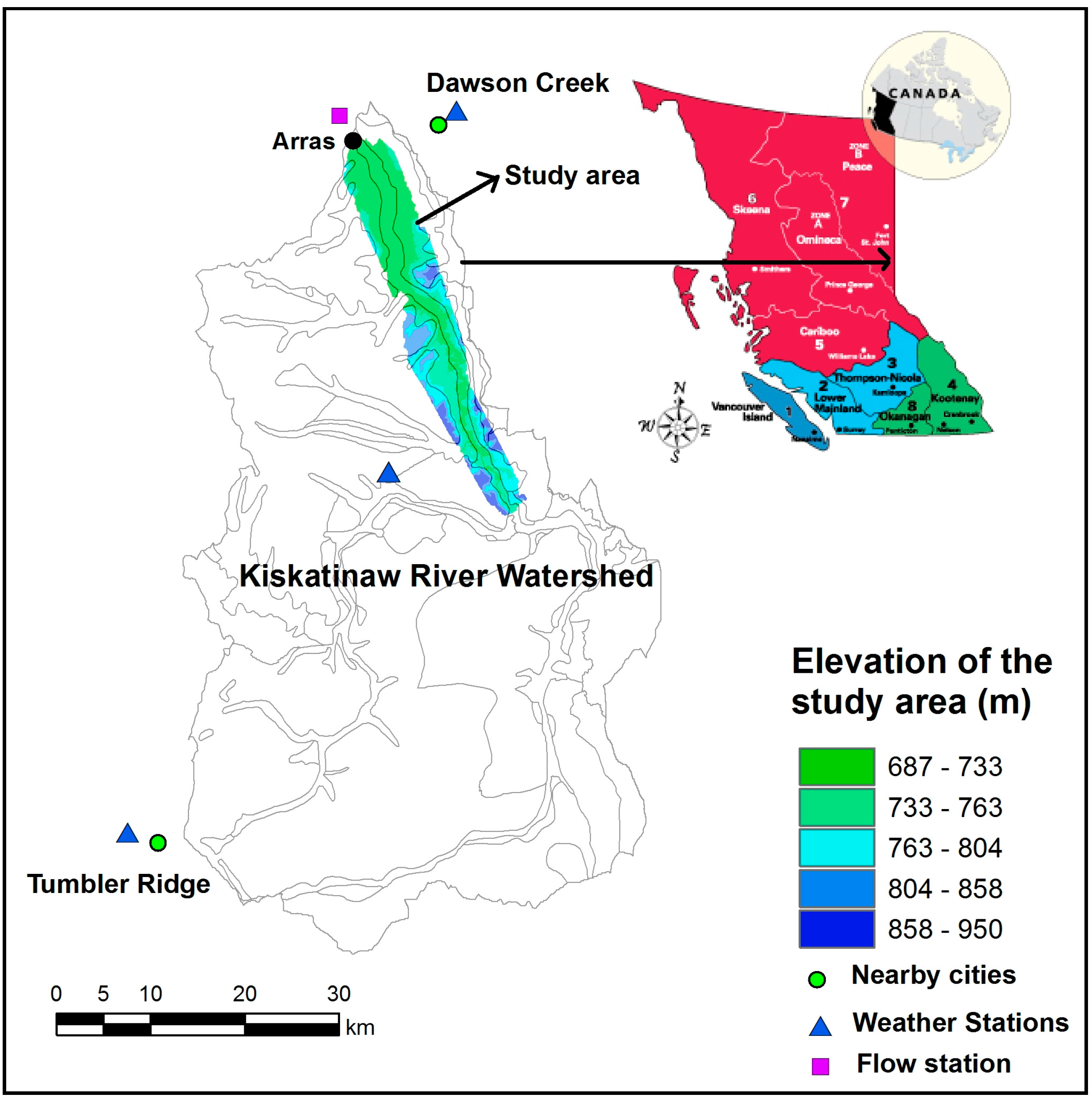
2. Details of Study Area

The study area (213.82 km²) is located along the main river of the Kiskatinaw River Watershed (KRW) in the Peace Region of north-eastern British Columbia, Canada (Figure 1). The City of Dawson Creek has been extracting water from Kiskatinaw River for drinking purposes since the mid-1940s [13]. In addition, the drinking water intake of the water supply system for Dawson Creek is situated at Arras in the study area. The study area has an elevation ranging from 687 m to 950 m. Clay loam, silt loam and sandy loam cover 91%, 6%, and 3%, respectively of the study area [14]. The average slope in the study area is 7.8%. Forest, forest clear cut, agriculture, wetland, water, and built up area cover 68%, 18.7%, 8%, 2%, 1.8%, and 1.5%, respectively, of the study area (Figure 2) [14].

The KRW is a rain dominated hydrologic system. On average, it receives an annual precipitation of 499 mm, consisting of 320 mm of rainfall, and 179 mm of snow [13]. During the last 40 years, the City of Dawson Creek has experienced steady water demand growth with an average annual growth rate of about 3.2%. In addition, the KRW has many other values, such as timber harvesting, agriculture, oil and gas, recreation, wildlife, and potential mineral resources development [13]. In particular, a large and increasing scale of timber harvesting, oil and gas exploration/production, and agricultural activities in recent years have created growing concerns of water to various users. Therefore, it is necessary to conduct the study of climate change induced precipitation effects on water resources in the study area for developing future water resources management and water allocation plan.

3. Materials and Methodology

3.1. Data Collection

Digital elevation model (DEM) data on a 13.74 m by 23.81 m resolution grid was collected from Canadian Digital Elevation Data (CDED) [15]. Observed hourly precipitation, temperature and other meteorological data were collected from nearby three weather stations in the KRW, and those were averaged by using arithmetic method to get daily distribution of those parameters for 2000 to 2011. Stream flow data at Arras site (i.e., outlet of study area) during 2006–2011 were collected from nearby Water Survey of Canada station. Land use and land cover map (30 m by 30 m grid) for the study area in 2010 was generated from Paul’s [16] results using Arc GIS. In this study, land use and land cover map in 2010 was kept constant to all other years due to lack of maps on those years for maintaining simplicity for model calibration and validation as well as future climate change effects on water resources.

3.2. GSSHA Hydrological Model Development

GSSHA is a physically based, distributed parameter, and structured grid based hydrologic model [17]. It simulates major processes for example, spatially and temporally varying precipitation, snowfall accumulation and melting, precipitation interception, infiltration, evapotranspiration, surface runoff routing, unsaturated zone soil moisture accounting, saturated groundwater flow, overland flow, sediment erosion. Each process simulated has its own time-step and associated update time. During each time-step, the update time is compared with the current model time, and when they match, the process is updated and the information is transferred to dependent processes. This formulation allows the simultaneous simulation of processes that have dissimilar response times for example, overland flow, evapotranspiration, and lateral groundwater flow. The details of GSSHA can be found in Downer [17]. In this study, GSSHA model was used because it is a watershed based hydrologic model and it can simulate stream flow, groundwater discharge and surface runoff under climate change scenarios. This model was also used in hydrologic studies in different types of watersheds [18,19,20,21,22]. The following data are required to develop a GSSHA model:

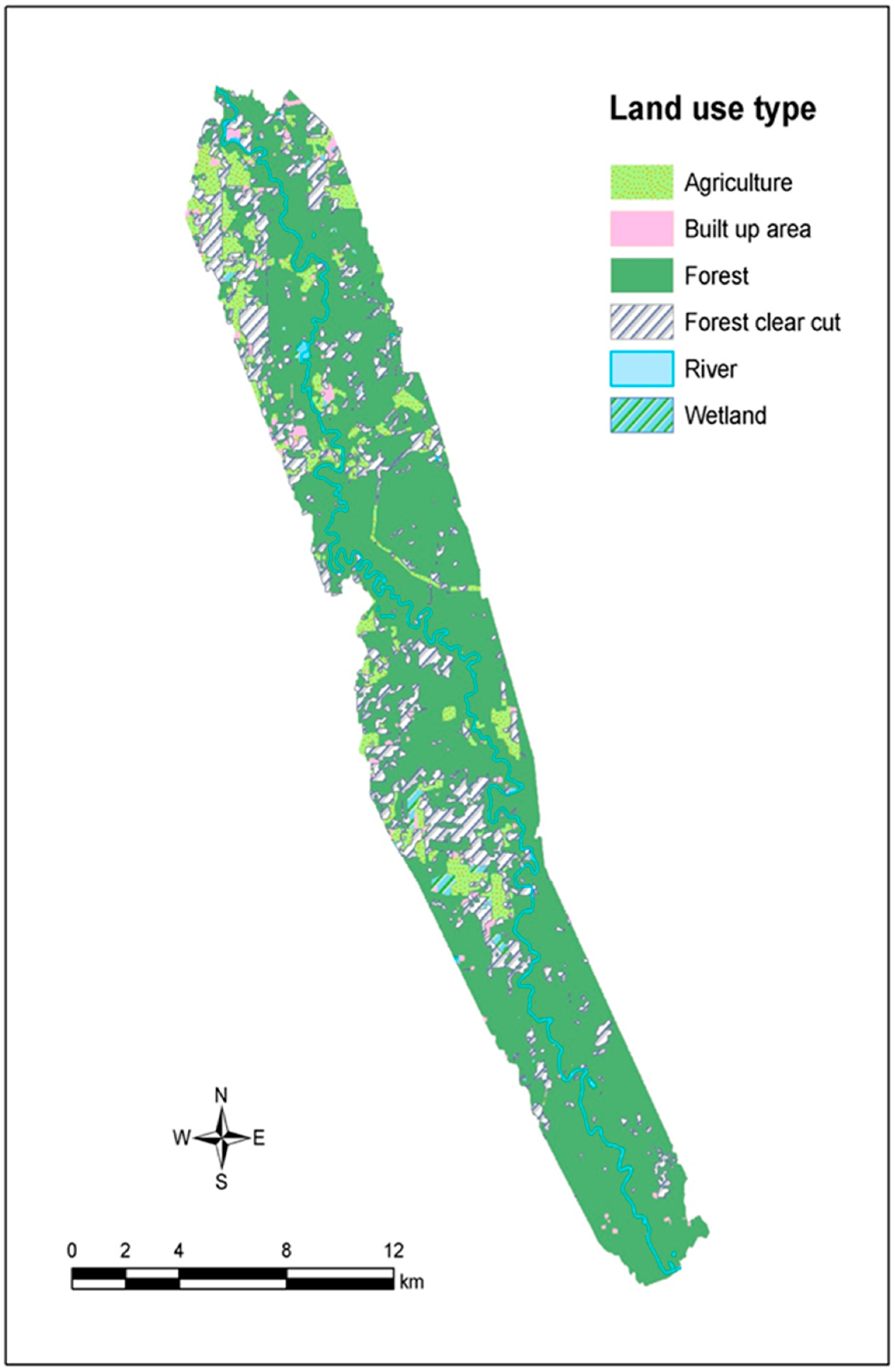
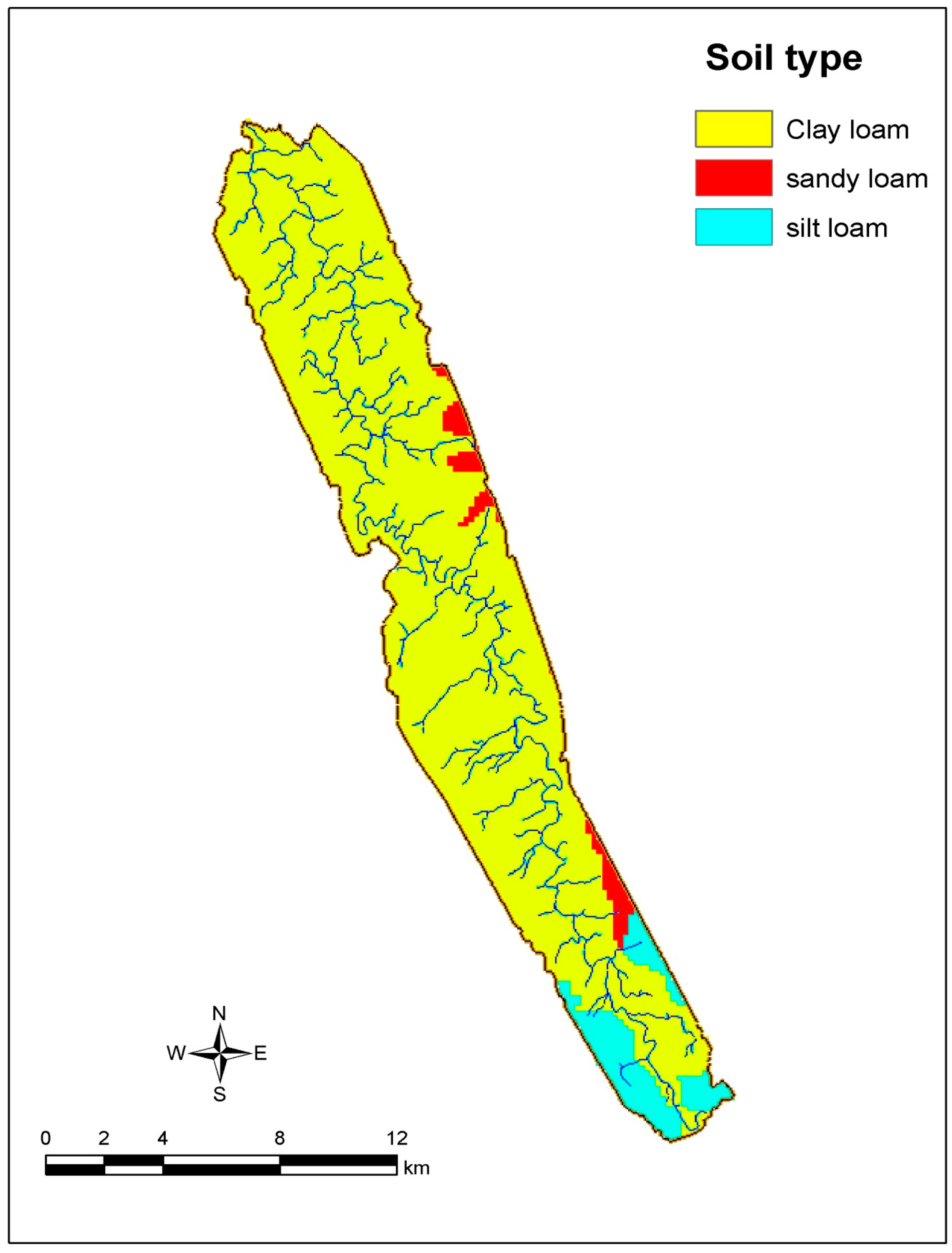
• Watershed specific data (e.g., elevation, channel geometry, soil type, land use/land cover), which were obtained from Geographic Information Systems (GIS) databases, satellite images, soil survey reports, and field observations.
• Precipitation and temperature data, and other meteorological data (e.g., barometric pressure, relative humidity, wind speed, direct and global radiation), which were collected from available weather stations in the KRW.
• Stream flow data, which was collected from the nearby Water Survey of Canada station.
• Groundwater level data which were collected from groundwater monitoring network in the KRW.
• Channel cross section data which was approximated based on field survey data.

In the GSSHA model, snowfall accumulation is considered when precipitation occurs during an air temperature of below 0 °C. In this model, infiltration is calculated using the Green and Ampt infiltration with redistribution (GAR) method [23]. Overland flow routing is simulated using the alternating direction explicit (ADE) finite difference method, and channel routing is simulated using an explicit solution of the diffusive wave equation. Water flux between the stream and the saturated groundwater is calculated based on Darcy’s law. During GSSHA model development, the Watershed Modeling System (WMS) Version 8.4, a graphically-based software environment, was used for delineating watershed, importing land use map and segmentation, defining segment cross section parameters, developing reach segment parameters, defining climate and meteorological input time series data. Using WMS, a 2-D GSSHA grid with spatial resolution of 30 m by 30 m was chosen for simulation based on available grid sized DEM and land use maps. Three index maps were prepared for parameter assignment at the grid level: a soil type index map (Figure 3), a land use index map, and a combined land use and soil type index map. In addition to these maps, aquifer bottom and initial groundwater table maps were prepared to simulate water resources (i.e., stream flow and groundwater discharge) using GSSHA model. Initial groundwater table map in the study area was prepared using inverse distance weighted (IDW) interpolation method and observed groundwater table data collected from groundwater monitoring network consisting of 26 piezometers in the KRW. Aquifer (unconfined) bottom map was prepared using IDW interpolation method and bore log data of a few existing wells in the KRW and its surrounding area collected from the database of British Columbia Water Resources Atlas [24]. Before using these collected groundwater table data, barometric pressure correction was applied on those data because groundwater table fluctuates by atmospheric pressure with altitude change [25]. The barometric pressure correction was made according to Solinst’s technical guidelines [26]. The barometric pressure data were collected from the three nearby weather stations because barologger was not used in this study.

Figure 3. Soil type index map of the study area.

Figure 3. Soil type index map of the study area.

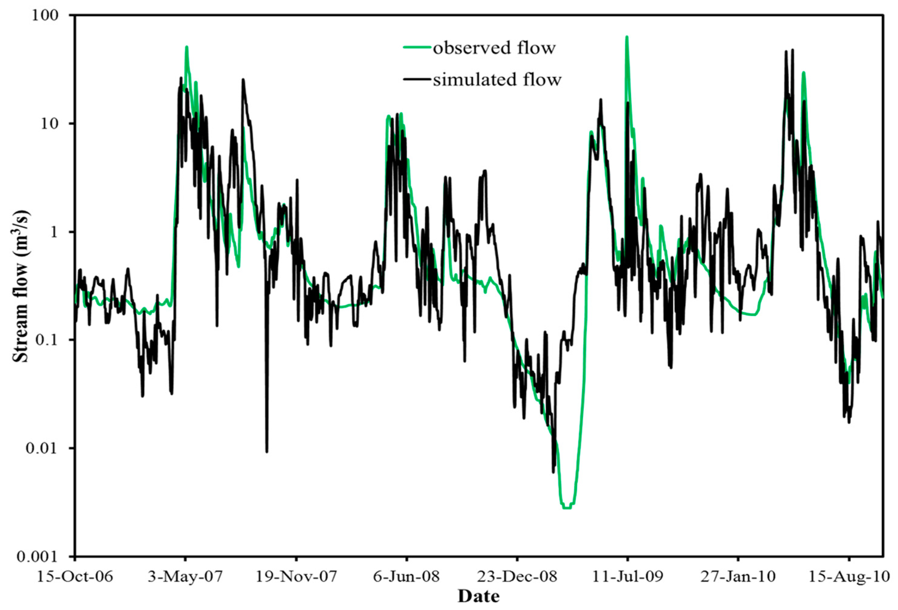
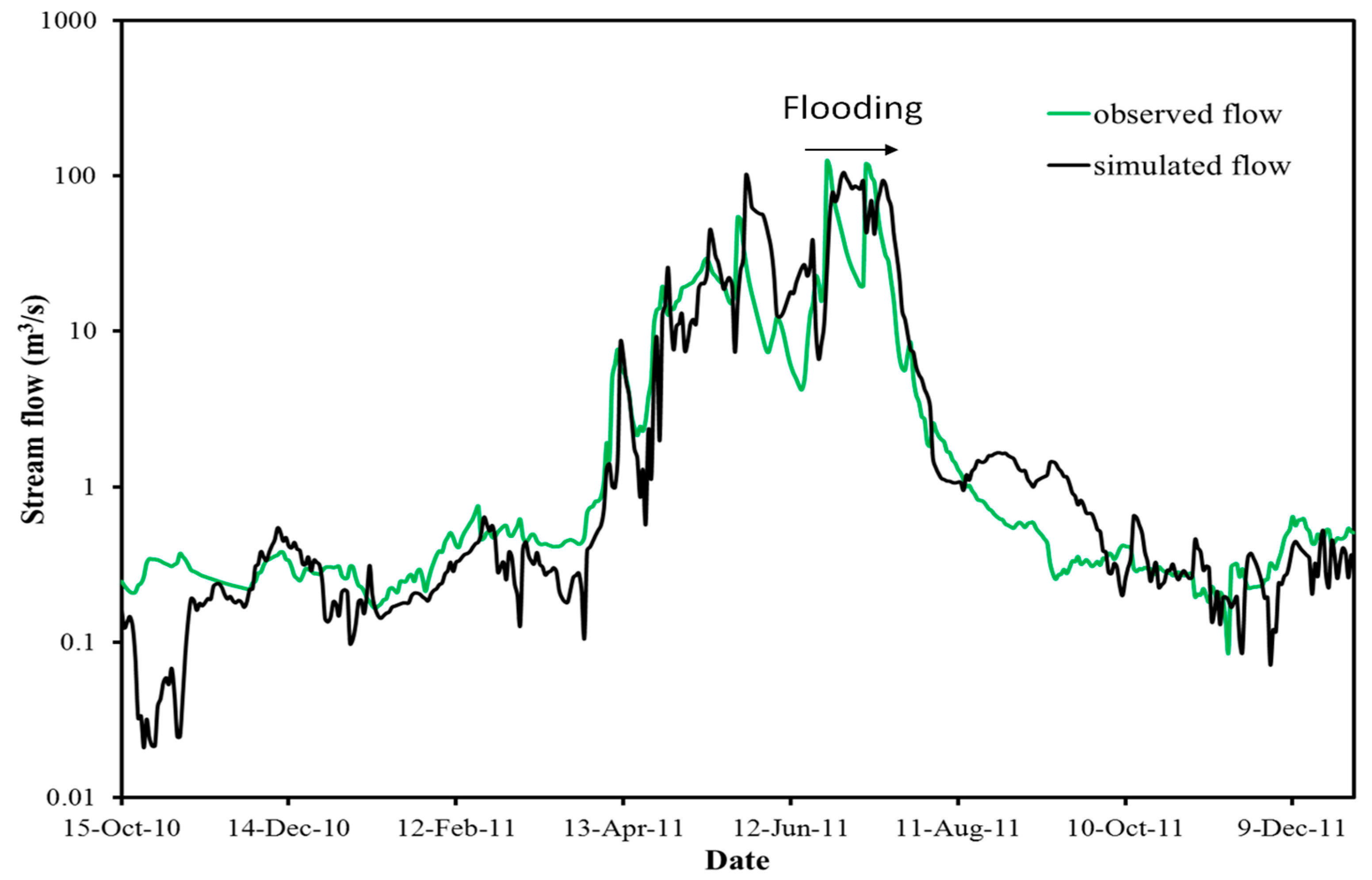
3.3. Model Calibration and Validation

Two types of boundary conditions were considered in GSSHA model; one is for a groundwater boundary condition around the perimeter of the study area, and the other is also a groundwater boundary condition for streams. For the groundwater boundary condition around the perimeter of the study area, no flow boundary condition was assumed based on previous studies results [27]. For stream routing, flux river was chosen as groundwater boundary condition for streams because a significant amount of water goes into the subsurface (groundwater) flow from the stream network. After developing the model, it was calibrated using automated calibration. The developed GSSHA model was calibrated using measured stream flow by changing soil parameters (i.e., hydraulic conductivity, and porosity), overland surface roughness, channel roughness, overland retention depth, initial soil moisture, and soil moisture depth. The coefficient of determination (R²), and coefficient of efficiency (NSE: Nash-Sutcliffe efficiency) were used to evaluate the goodness-of-fit of this hydrologic model. A simulation time step of 1 min was used for calibration and validation based on the temporal convergence study of observed and simulated stream flows at the outlet of the study area. Due to limited observed stream flow data, the model calibration was performed from 15 October 2006 to 15 October 2010, and validation was performed from 15 October 2010 to 31 December 2011. It is to be noted that there was a flood in 2011, and model validation was performed during 2011 to assess the performance of the model, and model calibration was performed in normal precipitation years. During calibration of the developed model (Figure 4), R² = 0.62, and NSE = 0.59 were found. Santhi et al. [28] and Van Liew et al. [29] reported that R² value greater than 0.5 is considered as acceptable for model evaluation. The United States Environmental Protection Agency (US EPA) [30] also stated that R² value between 0.6 and 0.7 shows fair performance for hydrologic models. Based on these evaluation statistics guidelines, the developed model fulfills all the criterion. During validation (Figure 5), R² = 0.65, and NSE =0.61 were found.

Figure 4. Comparison of observed and simulated stream flows with the Gridded Surface Subsurface Hydrologic Analysis (GSSHA) model at the outlet of the study area during the calibration period.

Figure 4. Comparison of observed and simulated stream flows with the Gridded Surface Subsurface Hydrologic Analysis (GSSHA) model at the outlet of the study area during the calibration period.

Figure 5. Comparison of observed and simulated stream flows with the GSSHA model at the outlet of the study area during the validation period.

Figure 5. Comparison of observed and simulated stream flows with the GSSHA model at the outlet of the study area during the validation period.

3.4. Generation of Future Climate Scenarios

Precipitation and temperature for the long-term period (2020–2040) were downscaled from CRCM 4.2 (Canadian Regional Climate Model) modeling outputs of the CCCma (Canadian Centre for Climate Modeling and Analysis) using the delta change method under two types of greenhouse gas (GHG) emission scenarios of SRES (Special Report on Emissions Scenarios) of the Intergovernmental Panel on Climate Change (IPCC) [31], namely the A2 and B1 scenarios. The A2 scenario describes a heterogeneous world, which is characterized by self-resilient nations, continuously increasing in population, and with a regionally oriented economic development. The A2 scenario was chosen because it represents regional economic development, and in the KRW, the large-scale shale gas exploration/production activities began in 2005, and enhances regional economy [32]. On the other hand, the B1 scenario describes a more integrated and ecologically friendly world, which is characterized by a smaller population and global solutions to economic, social and environmental stability. The B1 scenario was chosen because it describes a more integrated and environmental friendly world [31]. Long term scenarios of two decades were also used in a number of climate change impacts studies on water resources [33,34,35]. The output from the CRCM (45 km grid) is monthly means for the A2 and B1 GHG emission scenarios. These monthly mean values were distributed as daily value for every day in the particular month using delta change downscaling method, which is a commonly applied method to cope with biases when using climate model outputs in hydrological impact studies at catchment or sub-watershed scale [36,37]. It is a simple way of transferring the change in a meteorological variable, as simulated by the climate model, to an observed data set to create a scenario climate data set. A number of studies used the delta change method for hydrological impact assessments in Scandinavia [2,38,39,40,41]. In this study, the monthly delta change values for precipitation and temperature were determined for the watershed scale from the CRCM 4.2 simulation outputs because these outputs are from a 45-km horizontal grid-size mesh [42]. For each scenario, 3 CRCM simulations outputs were ensembled as mean for assessing the average impacts of climate change on water resources. Similar approach was used in various hydrological studies [43,44,45,46]. Absolute changes were used for temperature because it is a variable state and not a flux, whereas the relative change factors were applied for precipitation because it is a flux [47]. For precipitation, the delta change method can be described as follows:

$$P_{\Delta }(i,j)={\Delta }_P\left(j\right)*P_{obs}(i,j) ,i=1,2,\dots 31; j=1,2,\dots 12$$

(1)

where $P_{\Delta }$ is the precipitation input for the future hydrological scenario simulation, $P_{obs}$ is the observed precipitation in the historical period, (i, j) stand for day and month, respectively, and $P_{\Delta }$ is the change in precipitation, which can be calculated by:

$${\Delta }_P\left(j\right)=\frac{\overline{P}scen \left(j\right)}{\overline{P}ctrl \left(j\right)},j=1,2,\dots 12$$

(2)

where $\overline{P}ctrl \left(j\right)$ is the mean daily precipitation for month j and it is calculated as the mean of precipitation of all days in month j for all 12 years of the reference period, and $\overline{P}scen \left(j\right)$ is the mean daily precipitation for month j of each particular year from 2020 to 2040. The indices “scen” and “ctrl” stand for the scenario period (2020–2040) and the control period (2000–2011), respectively. This led to 12 monthly delta change values for each year from 2020 to 2040, and they were used to adjust the observed daily precipitation within the individual months for future precipitation input.

For temperature; the procedure of delta change method is as follows:

$$T_{\Delta }(i,j)=T_{obs}(i,j)+{\Delta }_T\left(j\right) ,i=1,2,\dots 31; j=1,2,\dots 12$$

(3)

where ${\text{T}}_{\Delta }$ is the temperature input for the future hydrological scenario simulation, $T_{obs}$ is the observed temperature in the historical period, (i, j) stand for day and month, respectively, and ${\Delta }_{\text{T}}$ is the change in temperature. This ${\Delta }_{\text{T}}$ value is calculated by Equation (4).

$${\Delta }_T \left(j\right)= {\overline{T}}_{scen} \left(j\right)- {\overline{T}}_{ctrl} \left(j\right) ,j=1,2,\dots 12$$

(4)

where ${\overline{\text{T}}}_{\text{ctrl}}\left(\text{j}\right)$ is the mean daily temperature for month j and it is calculated as the mean of temperature of all days in month j for all 12 years of the reference (i.e., control) period; ${\overline{T}}_{\text{scen}}\left(\text{j}\right)$ is the mean daily temperature for month j of each particular year from 2020 to 2040. The indices “scen” and “ctrl” stand for the scenario period (2020–2040) and the control period (2000–2011), respectively.

3.5. Estimation of Groundwater Discharge and Surface Runoff

Groundwater discharge and surface runoff were estimated during the reference period and both future climate change scenarios. Groundwater discharge during the reference period was estimated using the PART base flow separation program of the USGS, which uses only observed stream flow data [48]. This program estimates daily base flow by considering it to be equal to stream flow on days that fit a requirement of antecedent recession, and then linearly interpolating it for other days in the stream flow record. Based on these daily values, the mean monthly groundwater discharge was calculated. Mean monthly surface runoff during the reference period was calculated by subtracting mean monthly groundwater discharge from mean monthly stream flow. On the other hand, groundwater discharge and surface runoff during 2020–2040 in both scenarios were estimated using the developed GSSHA model. The GSSHA model estimates monthly total volume of groundwater discharge and surface runoff, and based on those values the mean monthly groundwater discharge and surface runoff were calculated [49].

4. Results and Discussions

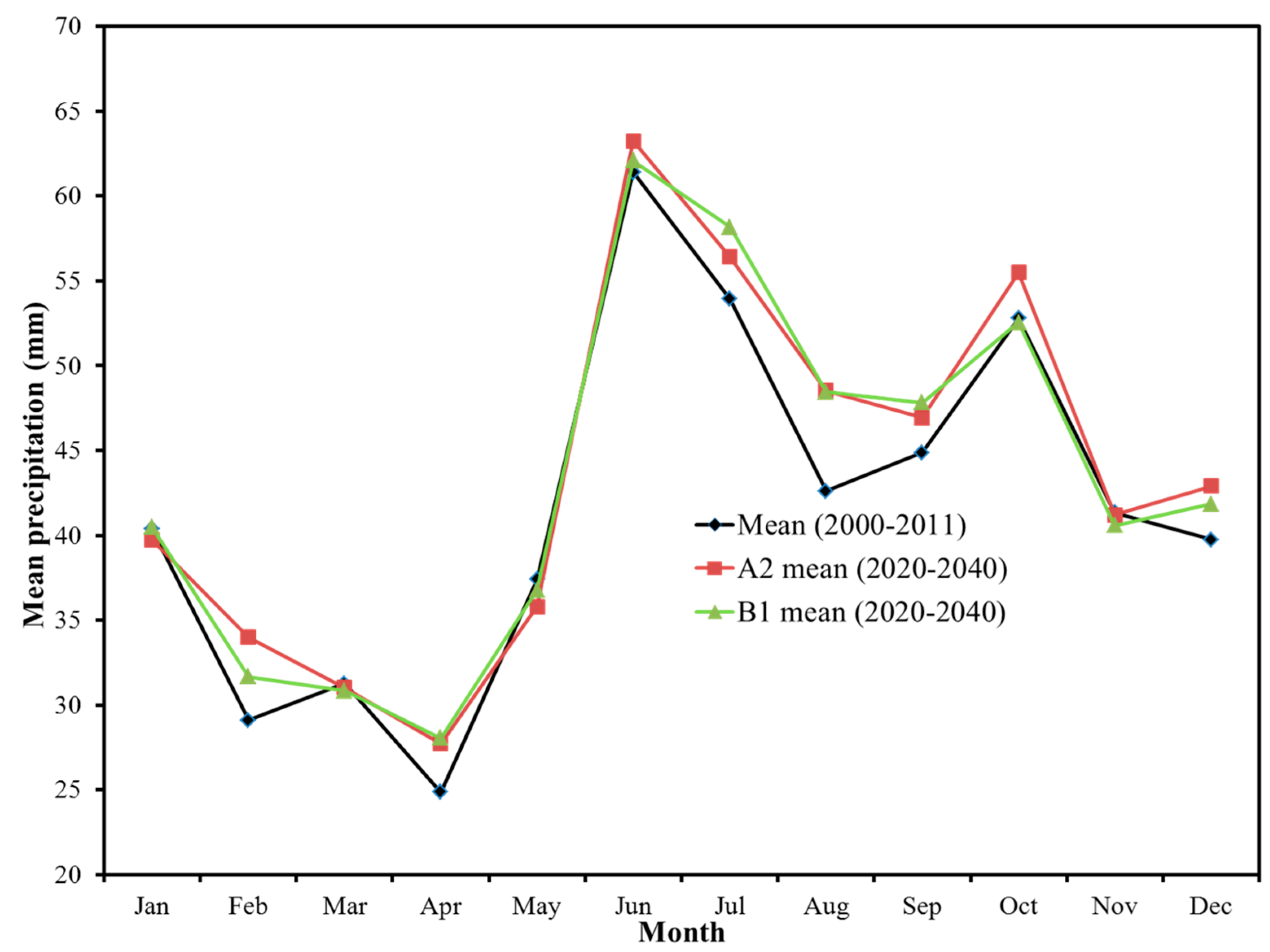
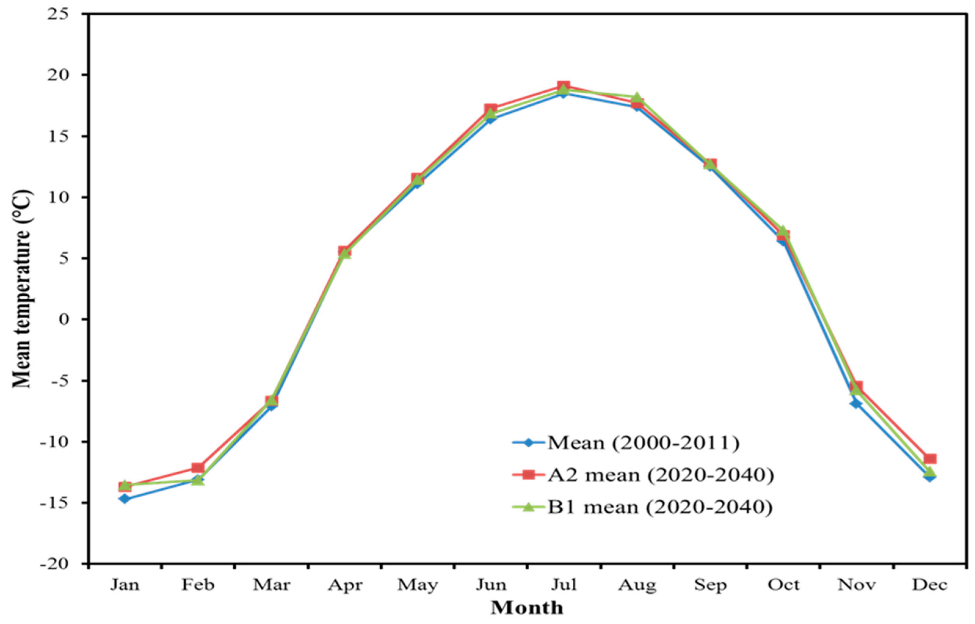
4.1. Results of Climate Change

From the comparison of projected mean monthly precipitations in both scenarios from 2020 to 2040 with respect to the reference period from 2000–2011 (Figure 6), it is found that the peak monthly precipitation in both scenarios is expected in June, and shows the similar trend of the mean monthly precipitations from 2000–2011. The mean monthly precipitations are higher in most of the months under the A2 scenario than under the B1 scenario. The highest and lowest seasonal precipitations in both scenarios from 2020–2040 are expected in summer (June–August) and spring (March–May), respectively (Table 1). The mean seasonal precipitations are also expected to increase in 2020–2040 in both scenarios with respect to the mean seasonal precipitations from 2000 to 2011 (Table 2) due to the anthropogenic increases in the atmospheric concentrations of greenhouse gases [31,50]. It is also found that the increase of mean precipitation is greater in the summer (9.5% in A2 and 4.5% in B1 scenarios) than that in the winter (3% in A2 and 4.5% in B1 scenarios). Similar types of increased precipitation patterns were predicted in the Peace Region in previous studies [7,12]. Similarly, the mean annual precipitation is expected to increase in 2020–2040 as compared to the period from 2000–2011. The mean annual precipitation from 2020 to 2040 under the A2 and B1 scenarios is expected to be 525 mm (σ = 19 mm) and 516 mm (σ = 22 mm), respectively, and these numbers are above the mean annual precipitation from 2000–2011 by 27 mm (5.5%) and 18 mm (3.5%), respectively.

Similar trends are expected in 2020–2040 when the projected mean monthly temperatures in both scenarios from 2020 to 2040 are compared to those from 2000–2011 (Figure 7). The mean seasonal temperatures are expected to increase in the long-term period. On average, the mean winter (December–February), spring (March–May), summer (June–August), and fall (September–November) temperatures from 2020 to 2040 under the A2 scenario are expected to be −12.42 °C (σ = 1.46 °C), 3.52 °C (σ = 0.69 °C), 18.03 °C (σ = 0.45 °C), and 4.55 °C (σ = 0.66 °C), respectively, which corresponds to an increase by 1.15 °C, 0.36 °C, 0.60 °C, and 0.55 °C, respectively, as compared to those from 2000–2011. On the other hand, under the B1 scenario, on average, the mean winter, spring, summer, and fall temperatures from 2020 to 2040 are expected to be −13.03 °C (σ = 1.15 °C), 3.40 °C (σ = 0.55 °C), 17.84 °C (σ = 0.62 °C), and 4.32 °C (σ = 0.49 °C), respectively, which corresponds to an increase by 0.52 °C, 0.24 °C, 0.40 °C, and 0.32 °C, respectively, as compared to those from 2000–2011. It is also found that the increase of mean temperature is greater in the winter (1.15 °C and 0.52 °C in A2 and B1 scenarios, respectively) than that in the summer (0.60 °C and 0.40 °C in A2 and B1 scenarios, respectively). Similar predictions were done in the Peace Region in previous studies [7,12]. Similarly, the mean annual temperature is also expected to increase in the long-term period. On average, the mean annual temperature from 2020 to 2040 under the A2 and B1 scenarios is expected to be 3.46 °C (σ = 0.60 °C) and 3.27 °C (σ = 0.41 °C), respectively, which is increased by 0.76 °C and 0.57 °C compared with that of 2000–2011, respectively. This occurs due to the anthropogenic increases in the atmospheric concentrations of greenhouse gases [31,50].

Figure 6. Comparison of projected mean monthly precipitations under the A2 and B1 scenarios from 2020 to 2040 with respect to the mean monthly precipitations of 2000–2011.

Figure 6. Comparison of projected mean monthly precipitations under the A2 and B1 scenarios from 2020 to 2040 with respect to the mean monthly precipitations of 2000–2011.

Figure 7. Comparison of projected mean monthly temperatures under the A2 and B1 scenarios from 2020 to 2040 with respect to those of 2000–2011.

Figure 7. Comparison of projected mean monthly temperatures under the A2 and B1 scenarios from 2020 to 2040 with respect to those of 2000–2011.

Table 1. Mean seasonal precipitations under the reference period (2000–2011) and A2 and B1 scenarios for the long-term period (2020–2040). The values within the parentheses are standard deviation among mean seasonal precipitations from 2020 to 2040. The unit of precipitation is mm.

Scenario	Winter	Spring	Summer	Fall
Reference	109	93	158	138
A2	112	95	173	145
	(12)	(11)	(17)	(9)
B1	114	96	165	141
	(13)	(9)	(18)	(13)

Table 1. Mean seasonal precipitations under the reference period (2000–2011) and A2 and B1 scenarios for the long-term period (2020–2040). The values within the parentheses are standard deviation among mean seasonal precipitations from 2020 to 2040. The unit of precipitation is mm.

Scenario	Winter	Spring	Summer	Fall
Reference	109	93	158	138
A2	112	95	173	145
	(12)	(11)	(17)	(9)
B1	114	96	165	141
	(13)	(9)	(18)	(13)

Table 2. Projected change in mean seasonal precipitations under the A2 and B1 scenarios for the long-term period (2020–2040) with respect to the mean seasonal precipitations under the reference period (2000–2011). The values within the parentheses are relative changes.

Scenario	Winter	Spring	Summer	Fall
A2	3 mm	2 mm	15 mm	7 mm
	(3%)	(2%)	(9.5%)	(5%)
B1	5 mm	3 mm	7 mm	3 mm
	(4.5%)	(3%)	(4.5%)	(2%)

Table 2. Projected change in mean seasonal precipitations under the A2 and B1 scenarios for the long-term period (2020–2040) with respect to the mean seasonal precipitations under the reference period (2000–2011). The values within the parentheses are relative changes.

Scenario	Winter	Spring	Summer	Fall
A2	3 mm	2 mm	15 mm	7 mm
	(3%)	(2%)	(9.5%)	(5%)
B1	5 mm	3 mm	7 mm	3 mm
	(4.5%)	(3%)	(4.5%)	(2%)

4.2. Results of Climate Change Effects on Water Resources

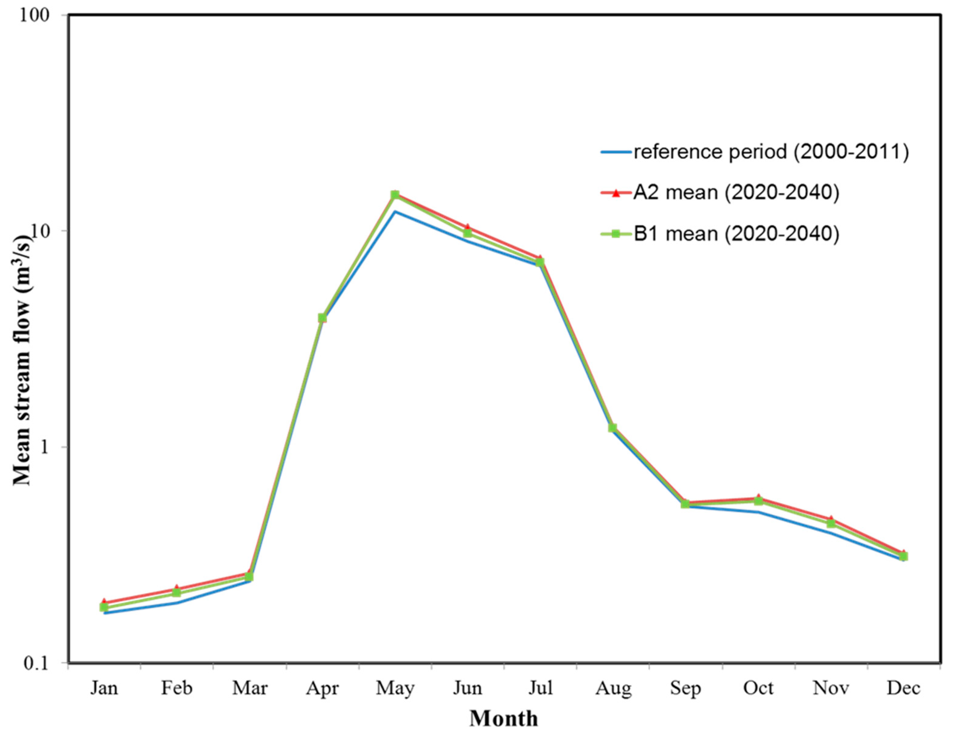
The simulated results were analyzed on a mean monthly basis. Figure 8 shows the comparison of mean monthly stream flow from 2020–2040 under climate change of A2 and B1 GHG emission scenarios with respect to the reference period (2000–2011). It is to be noted that the observed stream flow data from 2000 to 2011 were collected from nearby Water Survey of Canada station, and the data from 2006 to 2011 were used for calibration and validation, and the remaining period data were not used for calibration and validation because of lack of several monthly flow data in several years. These results show that the highest mean monthly stream flow occurs in May although the peak monthly precipitation occurs during June. This variation occurs because of snow melting, which starts during April, and increased evapotranspiration of forested area during June in the study area. The results also illustrate that the mean monthly stream flow from 2020–2040 is higher during most of the months under the A2 scenario than under the B1 scenario due to a higher amount of precipitation and temperature increase predicted under the A2 scenario. The highest and lowest mean monthly stream flows from 2020–2040 in both scenarios are expected to occur in May and January, respectively (Table 3). The mean monthly stream flow from 2020–2040 under the A2 and B1 scenarios are higher all the year than under the reference period (2000–2011) due to increased precipitation and temperature predicted under those scenarios with respect to the reference period. Therefore, climate change induced precipitation changes significantly influence the amount of mean monthly stream flow in the study area.

Figure 8. Comparison of mean monthly stream flow from 2020–2040 under climate change of A2 and B1 GHG emission scenarios with respect to the reference period (2000–2011).

Figure 8. Comparison of mean monthly stream flow from 2020–2040 under climate change of A2 and B1 GHG emission scenarios with respect to the reference period (2000–2011).

In terms of seasonal patterns, stream flow in both scenarios is expected to increase as compared to that under the reference period (Table 4). This occurs due to increased precipitation and temperature predicted in both scenarios as compared to the reference period. However, the major increase is expected under the A2 scenario due to higher amount of precipitation expected to occur. Therefore, the effect of climate change induced precipitation on the mean seasonal stream flow is significant. Consequently, the highest and lowest water extraction from the river, and allocation to the stakeholders for future water supply under the A2 scenario could be possible during summer and winter, respectively, due to the highest (i.e., on average 6.34 m³/s) and lowest (i.e., on average 0.24 m³/s) mean stream flow rates during summer and winter, respectively. On the other hand, in the B1 scenario, the highest and lowest water extraction from the river, and allocation to the stakeholders for future water supply could be possible during spring and winter, respectively, due to the highest (i.e., on average 6.27 m³/s) and lowest (i.e., on average 0.23 m³/s) mean stream flow rates during spring and winter, respectively. However, the development activities are continuously increasing in the study area and results in increasing water demand in future. Although the future water demand in the study area is unknown, this information would provide valuable information for the watershed manager for developing future water allocation plan in the study area.

Table 3. Mean monthly stream flow during the reference period (2000–2011) and A2 and B1 scenarios for the long-term period (2020–2040), and projected percent change in mean monthly stream flow in the A2 and B1 scenarios for the long-term period (2020–2040) with respect to that under the reference period (2000–2011).

Month	Stream Flow (m3/s) under Reference Period	Stream Flow (m3/s) under A2 Scenario	Percent Change under A2 Scenario	Stream Flow (m3/s) under B1 Scenario	Percent Change under B1 Scenario
January	0.17	0.19	11.7	0.18	5.5
February	0.19	0.22	15.8	0.21	9.5
March	0.24	0.26	8.3	0.25	4
April	3.85	3.93	2.1	3.97	3.1
May	12.28	14.78	20.3	14.58	15.8
June	8.97	10.35	15.3	9.73	7.8
July	6.9	7.43	7.6	7.2	4.1
August	1.18	1.23	4.2	1.22	3.2
September	0.53	0.55	3.8	0.54	1.9
October	0.5	0.58	16	0.56	10.7
November	0.4	0.46	15	0.44	9.1
December	0.3	0.32	6.7	0.31	3.3

Table 3. Mean monthly stream flow during the reference period (2000–2011) and A2 and B1 scenarios for the long-term period (2020–2040), and projected percent change in mean monthly stream flow in the A2 and B1 scenarios for the long-term period (2020–2040) with respect to that under the reference period (2000–2011).

Month	Stream Flow (m3/s) under Reference Period	Stream Flow (m3/s) under A2 Scenario	Percent Change under A2 Scenario	Stream Flow (m3/s) under B1 Scenario	Percent Change under B1 Scenario
January	0.17	0.19	11.7	0.18	5.5
February	0.19	0.22	15.8	0.21	9.5
March	0.24	0.26	8.3	0.25	4
April	3.85	3.93	2.1	3.97	3.1
May	12.28	14.78	20.3	14.58	15.8
June	8.97	10.35	15.3	9.73	7.8
July	6.9	7.43	7.6	7.2	4.1
August	1.18	1.23	4.2	1.22	3.2
September	0.53	0.55	3.8	0.54	1.9
October	0.5	0.58	16	0.56	10.7
November	0.4	0.46	15	0.44	9.1
December	0.3	0.32	6.7	0.31	3.3

Table 4. Mean seasonal stream flow during the reference period (2000–2011) and A2 and B1 scenarios during the long-term period (2020–2040). The values within the parentheses are relative changes. The unit of stream flow is m³/s.

Scenario	Winter	Spring	Summer	Fall
Reference period	0.22	5.46	5.68	0.48
A2	0.24	6.32	6.34	0.53
	(10%)	(16%)	(11%)	(11%)
B1	0.23	6.27	6.02	0.51
	(6%)	(15%)	(6%)	(8%)

Table 4. Mean seasonal stream flow during the reference period (2000–2011) and A2 and B1 scenarios during the long-term period (2020–2040). The values within the parentheses are relative changes. The unit of stream flow is m³/s.

Scenario	Winter	Spring	Summer	Fall
Reference period	0.22	5.46	5.68	0.48
A2	0.24	6.32	6.34	0.53
	(10%)	(16%)	(11%)	(11%)
B1	0.23	6.27	6.02	0.51
	(6%)	(15%)	(6%)	(8%)

On average, the mean annual stream flow during 2020–2040 in the A2 and B1 scenarios is expected to be 3.42 m³/s (σ = 0.09 m³/s), and 3.32 m³/s (σ = 0.08 m³/s), respectively. This variation occurs due to a higher precipitation and temperature increase predicted in the A2 scenario than the B1 scenario from 2020 to 2040. On average, the mean annual stream flow of the reference period (2000–2011) is approximately 2.96 m³/s. With respect to the mean annual stream flow of the reference period, the mean annual stream flow from 2020 to 2040 under the A2 and B1 scenarios is expected to increase by 15.5% and 12.1%, respectively, due to the increased precipitation and temperature predicted in both scenarios (Table 5). Similar projections were done for Williston reservoir in the Peace Region for the 2050s [51]. Therefore, changes in annual precipitation due to climate change also affect annual stream flow significantly. These results indicate that more annual water extraction from the river, and allocation to the stakeholders for future water supply could be possible under the A2 scenario than under the B1 scenario without causing a negative impact on regional groundwater level.

In addition to stream flow, simulation results show that groundwater discharge and surface runoff are also expected to increase in 2020–2040 in both scenarios due to increased precipitation (Table 5). However, surface runoff increased more compared to groundwater discharge because of the steep topography of the study area [52]. This increased surface runoff in both scenarios will result in increased nutrient concentrations in stream (e.g., Dissolved organic carbon (DOC) and nitrogen (DON)) that may promote excessive growth of habitat-choking algae by increasing soil erosion [53,54]. The increased soil erosion would also obstruct the river and its channel by changing the river morphology, and pollute the river water by transporting pesticide, herbicides, and fertilizers from the agricultural land via increased surface runoff [55]. Crop productivity would also be reduced due to increased soil erosion by changing the soil structure. These results demonstrate that under the B1 scenario those above mentioned impacts will be lower as compared to the A2 scenario due to lower surface runoff under the B1 scenario.

Table 5. Mean annual precipitation, temperature, stream flow, surface runoff, and groundwater discharge over the reference period (2000–2011) and A2 and B1 scenarios for the long-term period (2020–2040). The values within the parentheses are relative changes except for temperature, where absolute changes were calculated.

Scenario	Mean Annual precipitation (mm)	Mean Annual Temperature (°C)	Mean Annual Stream Flow (m3/s)	Mean Annual Groundwater Discharge (m3/s)	Mean Annual Surface Runoff (m3/s)
Reference	498	2.7	2.96	2.43	0.53
A2	525	3.46	3.42	2.55	0.87
	(5.5%)	(0.76)	(15.5%)	(5%)	(64.1%)
B1	516	3.27	3.32	2.51	0.81
	(3.5%)	(0.57)	(12.1%)	(3.3%)	(52.8%)

Table 5. Mean annual precipitation, temperature, stream flow, surface runoff, and groundwater discharge over the reference period (2000–2011) and A2 and B1 scenarios for the long-term period (2020–2040). The values within the parentheses are relative changes except for temperature, where absolute changes were calculated.

Scenario	Mean Annual precipitation (mm)	Mean Annual Temperature (°C)	Mean Annual Stream Flow (m3/s)	Mean Annual Groundwater Discharge (m3/s)	Mean Annual Surface Runoff (m3/s)
Reference	498	2.7	2.96	2.43	0.53
A2	525	3.46	3.42	2.55	0.87
	(5.5%)	(0.76)	(15.5%)	(5%)	(64.1%)
B1	516	3.27	3.32	2.51	0.81
	(3.5%)	(0.57)	(12.1%)	(3.3%)	(52.8%)

4.3. Uncertainties Regarding the Results of Climate Change Effects on Water Resources

Since future climate change scenarios contain uncertainty [56], uncertainty analysis of climate change should be incorporated in further studies to assess the average impact of climate change scenarios on water resources. Moreover, internal variability could also affect the patterns of climate change scenarios, which were not considered in this study. Therefore, the results obtained in this study should be considered as some trends and orders of magnitudes rather than exact predictions. In addition, different climate models may give different scenarios of future precipitation and temperature trends in the A2 and B1 GHG emission scenarios. Therefore, other climate models predicted precipitation and temperature should be used for comparing the results obtained from this study. Finally, different downscaling method (e.g., dynamic downscaling) could also be used to compare the results.

5. Conclusions

In this study, the changes in precipitation due to climate change of the A2 and B1 GHG emission scenarios for 2020–2040, and its effects on water resources were evaluated in a study area along the main river of the KRW in the Peace Region of BC, Canada. The Gridded Surface Subsurface Hydrologic Analysis (GSSHA) modeling system was used for this evaluation. The simulation results showed that climate change induced precipitation changes have significant effects on monthly, seasonal and annual stream flows in the study area. It also affects positively groundwater discharge and surface runoff. The results obtained from this study will provide useful information in the long-term period for seasonal and annual water extractions from the river and allocation to the stakeholders for future water supply, as well as for evaluating the ecological conditions of the stream, which will be beneficial to aquatic ecosystems. Therefore, this developed model is a useful tool for the planning of regional water resources management of the study area under climate change induced precipitation changes. The results also represent the symbolic scenarios of future climate change induced precipitation effects on water resources for other parts of the Peace Region.

References

1. National Aeronautics and Space Administration. Available online: http://atmospheres.gsfc.nasa.gov/climate/?section=135 (accessed on 22 November 2014).
2. Van Roosmalen, L.; Christensen, B.S.B.; Sonnenborg, T.O. Regional differences in climate change impacts on groundwater and stream discharge in Denmark. Vadose Zone J. 2007, 6, 554–571. [Google Scholar]
3. Dams, J.; Salvadore, E.; van Daele, T.; Ntegeka, V.; Willems, P.; Batelaan, O. Spatio-temporal impact of climate change on the groundwater system. Hydrol. Earth Syst. Sci. 2012, 16, 1517–1531. [Google Scholar] [CrossRef] [Green Version]
4. Bibi, U.M.; Kauk, J.; Balzter, H. Spatial-temporal variation and prediction of rainfall in northeastern Nigeria. Climate 2014, 2, 206–222. [Google Scholar] [CrossRef]
5. Cooley, K.R. Effects of CO2 induced climatic changes on snowpack and streamflow. Hydrol. Sci. J. 1990, 35, 511–522. [Google Scholar] [CrossRef]
6. Meenu, R.; Rehnana, S.; Mujumdar, P.P. Assessment of hydrologic impacts of climate change in Tunga-Bhadra river Basin, India with HEC-HMS and SDSM. Hydrol. Process. 2013, 27, 1572–1589. [Google Scholar] [CrossRef]
7. British Columbia Ministry of Forests and Range. Climate Change, Impacts, and Adaptation Scenarios: Climate Change and Forests and Range Management in British Columbia; Technical Report 045; British Columbia Ministry of Forests and Range: Victoria, BC, Canada, 2008. Available online: http://www.for.gov.bc.ca/hfd/pubs/Docs/Tr/Tr045.htm (accessed on 21 May 2013).
8. Eldorado Weather. Available online: http://www.eldoradocountyweather.com/canada/climate2/Vancouver%20International%20Airport.html (accessed on 21 November 2014).
9. McCarthy, J.J.; Canziani, O.F.; Leary, N.A.; Dokken, D.J.; White, K.S. Climate change 2001: Impacts, adaptation and vulnerability, intergovernmental panel on climate change. Int. J. Climatol. 2002, 22, 1285–1286. [Google Scholar] [CrossRef]
10. Kundzewicz, Z.W.; Mata, L.J.; Arnell, N.W.; Doell, P.; Jimenez, B.; Miller, K.; Oki, T.; Sen, Z.; Shiklomanov, I. The implications of projected climate change for freshwater resources and their management. Hydrol. Sci. J. 2008, 53, 3–10. [Google Scholar] [CrossRef]
11. Solomon, S.; Qin, D.; Manning, M.; Chen, Z.; Marquis, M.; Averyt, K.B.; Tignor, M.; Miller, H.L. Climate Change 2007: The Physical Science Basis, Contribution of Working Group I to the Fourth Assessment Report of the IPCC; Cambridge University Press: Cambridge, UK, 2007. [Google Scholar]
12. Chillborne Environmental. BC’s Peace River Valley and Climate Change. Available online: http://www.ceaa.gc.ca/050/documents/p63919/98108E.pdf (accessed on 6 November 2014).
13. Dobson Engineering Ltd.; Urban Systems Ltd. Kiskatinaw River Watershed Management Plan. Available online: http://www.dawsoncreek.ca/cityhall/departments/water/watershed/background-watershed-management-plans/ (accessed on 18 November 2014).
14. Saha, G.C. Groundwater-Surface Water Interaction under the Effects of Climate and Land Use Changes. Ph.D. Thesis, University of Northern British Columbia, Prince George, BC, Canada, 2014. [Google Scholar]
15. GeoBase. Available online: http://www.geobase.ca (accessed on 15 January 2014).
16. Paul, S.S. Analysis of Land Use and Land Cover Change in Kiskatinaw River Watershed: A Remote Sensing, GIS & Modeling Approach. Master Thesis, University of Northern British Columbia, Prince George, BC, Canada, 2013. [Google Scholar]
17. Downer, C.W. Identification and Modeling of Important Stream Flow Producing Processes in Watersheds. Ph.D. Thesis, University of Connecticut, Mansfield, CT, USA, 2002. [Google Scholar]
18. Downer, C.W.; Ogden, F.L. GSSHA: A model for simulating diverse streamflow generating processes. J. Hydrol. Eng. 2004, 9, 161–174. [Google Scholar] [CrossRef]
19. Downer, C.W.; Ogden, F.L. Prediction of runoff and soil moistures at the watershed scale: Effects of model complexity and parameter assignment. Water Resour. Res. 2004, 39. [Google Scholar] [CrossRef]
20. Sharif, H.O.; Ogden, F.L.; Krajewski, W.F.; Xue, M. Statistical analysis of radar-rainfall error propagation. J. Hydrometeorol. 2004, 5, 199–212. [Google Scholar] [CrossRef]
21. Sharif, H.O.; Yates, D.; Roberts, R.; Mueller, C. The use of an automated now-casting system to forecast flash floods in an urban watershed. J. Hydrometeorol. 2006, 7, 190–202. [Google Scholar] [CrossRef]
22. Swain, N.; Christensen, S.; Latu, K.; Jones, N.; Nelson, E.; Williams, G. A geospatial relational data model for ingesting GSSHA computational models: A step toward two-dimensional hydrologic modeling in the cloud. World Environ. Water Resour. Congr. 2013, 201, 2716–2725. [Google Scholar]
23. Ogden, F.L.; Saghafian, B. Green and ampt infiltration with redistribution. J. Irrig. Drain. Eng. 1997, 123, 386–393. [Google Scholar] [CrossRef]
24. British Columbia Ministry of Environment. Available online: http://www.env.gov.bc.ca/wsd/data_searches/wrbc/ (accessed on 10 August 2014).
25. McWhorter, D.B.; Sunada, D.K. Ground-Water Hydrology and Hydraulics; LLC.: Fort Collins, CO, USA, 1977. [Google Scholar]
26. Solinst. Available online: http://www.solinst.com (accessed on 20 May 2014).
27. Kala Groundwater Consulting Ltd. Groundwater Potential Evaluation Dawson Creek, British Columbia. Available online: http://www.dawsoncreek.ca/wordpress/wpcontent/uploads/watershed/2001DCk_Kala_GWPotential.pdf (accessed on 18 June 2014).
28. Santhi, C.; Arnold, J.G.; Williams, J.R.; Dugas, W.A.; Srinivasan, R.; Hauck, L.M. Validation of the SWAT model on a large river basin with point and nonpoint sources. J. Am. Water Resour. Assoc. 2001, 37, 1169–1188. [Google Scholar] [CrossRef]
29. Van Liew, M.W.; Arnold, J.G.; Garbrecht, J.D. Hydrologic simulation on agricultural watersheds: Choosing between two models. Trans. Am. Soc. Agric. Eng. 2003, 46, 1539–1551. [Google Scholar] [CrossRef]
30. US EPA. Lecture#5: Hydrological Processes, Parameters and Calibration. BASINS 4 Lectures, Data Sets and Exercises; United States Environmental Protection Agency: Washington, DC, USA, 2007.
31. IPCC. Emission Scenarios; IPCC Special Report; Cambridge University Press: Cambridge, UK, 2000; p. 570. [Google Scholar]
32. British Columbia Ministry of Energy and Mines. The Status of Exploration and Development Activities in the Montney Play Region of Northern BC. Available online: http://www.offshore-oilandgas.gov.bc.ca/OG/oilandgas/petroleumgeology/UnconventionalGas/Documents/C%20Adams.pdf (accessed on 19 December 2013).
33. Ashraf Vaghefi, S.; Mousave, S.J.; Abbaspour, K.C.; Srinivasan, R.; Yang, H. Analysis of the impact of climate change on water resources components, drought and wheat yield in semiarid regions: Karkheh River Basin in Iran. Hydrol. Process. 2014, 28, 2018–2032. [Google Scholar] [CrossRef]
34. Roy, L.; Leconte, R.; Brissette, F.P.; Marche, C. The impact of climate change on seasonal floods of a southern Quebec River Basin. Hydrol. Process. 2001, 15, 3167–3179. [Google Scholar] [CrossRef]
35. Yang, H.; Faramarzi, M.; Abbaspour, K.C. Assessing freshwater availability in Africa under the current and future climate with focus on drought and water scarcity. In Proceedings of the 20th International Congress on Modeling and Simulation, Adelaide, Australia, 1–6 December 2013.
36. Hay, L.E.; Wilby, R.L.; Leavesley, G.H. A comparison of delta change and downscaled GCM scenarios for three mountainous basins in the United States. J. Am. Water Resour. Assoc. 2000, 36, 387–398. [Google Scholar] [CrossRef]
37. Xu, C.Y.; Widen, E.; Halldin, S. Modeling hydrological consequences of climate change—Progress and challenges. Adv. Atmos. Sci. 2005, 22, 789–797. [Google Scholar] [CrossRef]
38. Andreasson, J.; Bergström, S.; Carlsson, B.; Graham, L.P.; Lindström, G. Hydrological change—Climate change impact simulation for Sweden. J. Hum. Environ. 2004, 33, 228–234. [Google Scholar]
39. Bergström, S.; Carlsson, B.; Gardelin, M.; Lindström, G.; Pettersson, A.; Rummukainen, M. Climate change impacts on runoff in Sweden—Assessments by global climate models, dynamical downscaling and hydrological modeling. Clim. Res. 2001, 16, 101–112. [Google Scholar] [CrossRef]
40. Graham, L.P. Climate change effects on river flow to the Baltic Sea. J. Hum. Environ. 2004, 33, 235–241. [Google Scholar]
41. Graham, L.P.; Andréasson, J.; Carlsson, B. Assessing climate change impacts on hydrology from an ensemble of regional climate models, model scales and linking methods—A case study on the Lule River basin. Clim. Change 2007, 81, 293–307. [Google Scholar] [CrossRef]
42. Bergeron, G.; Laprise, L.; Caya, D. Formulation of the Mesoscale Compressible Community (MC2) Model; Internal Report from Cooperative Center for Research in Mesometeorology: Montréal, QC, Canada, 1994; p. 165. [Google Scholar]
43. Scibek, J.; Allen, D.M. Modeled impacts of predicted climate change on recharge and groundwater levels. Water Resour. Res. 2006, 42. [Google Scholar] [CrossRef]
44. Vansteenkiste, T.; Tavakoli, M.; Ntegeka, V.; Willems, P.; de Smedt, F.; Batelaan, O. Climate change impact on river flows and catchment hydrology: A comparison of two spatially distributed models. Hydrol. Process. 2012, 27, 3649–3662. [Google Scholar] [CrossRef]
45. Nyenje, P.M.; Batelaan, O. Estimating the effects of climate change on groundwater recharge and baseflow in the upper Ssezibwa catchment, Uganda. Hydrol. Sci. J. 2009, 54, 713–726. [Google Scholar] [CrossRef]
46. Li, L.; Xu, H.; Chen, X.; Simonovic, S.P. Streamflow forecast and reservoir operation performance assessment under climate change. Water Resour. Manag. 2010, 24, 83–104. [Google Scholar] [CrossRef]
47. Van Roosmalen, L.; Christensen, J.H.; Butts, M.; Jensen, K.H.; Refsgaard, J.C. An intercomparison of regional climate model data for hydrological impact studies in Denmark. J. Hydrol. 2010, 380, 406–419. [Google Scholar] [CrossRef]
48. Rutledge, A.T. Computer programs for describing the recession of ground-water discharge and for estimating mean ground-water recharge and discharge from streamflow data—Update. U.S. Geological Survey: Reston, VA, USA, 1998; p. 43. [Google Scholar]
49. Downer, C.W.; Ogden, F.L. Gridded Surface Subsurface Hydrologic Analysis (GSSHA) User’s Manual; Coastal and Hydraulics Laboratory: Vicksburg, MS, USA, 2006; p. 207. [Google Scholar]
50. IPCC. Climate Change 2007: The Physical Science Basis, Contribution of working Group I to the 4th assessment report (AR4) of the Intergovernmental Panel on Climate Change; Cambridge University Press: Cambridge, UK, 2007; p. 996. [Google Scholar]
51. Hydro, B.C. Potential Impacts of Climate Change on BC Hydro’s Water Resources. Available online: https://www.bchydro.com/content/dam/hydro/medialib/internet/documents/about/climate_change_report_2012.pdf (accesses on 15 January 2015).
52. Vivoni, E.R.; Entekhabi, D.; Bras, R.L.; Ivanov, V.Y. Controls on runoff generation and scale-dependence in a distributed hydrologic model. Hydrol. Earth Syst. Sci. 2007, 11, 1683–1701. [Google Scholar] [CrossRef]
53. Price, K.; Leigh, D.S. Morphological and sedimentological responses of streams to human impact in the southern Blue Ridge Mountains, USA. Geomorphology 2006, 78, 142–160. [Google Scholar] [CrossRef]
54. Leigh, D.S. Hydraulic geometry and channel evolution of small streams in the Blue Ridge of western North Carolina. Southeast. Geogr. 2010, 50, 394–421. [Google Scholar]
55. Ontario Ministry of Agriculture, Food and Rural Affairs. Soil Erosion—Causes and Effects 2012. Available online: http://www.omafra.gov.on.ca/english/engineer/facts/12–053.pdf (accessed on 12 January 2015).
56. Christensen, J.H.; Christensen, O.B. A summary of the PRUDENCE model projections of changes in European climate by the end of this century. Clim. Change 2007, 81, 7–30. [Google Scholar] [CrossRef]