Changes in Average Annual Precipitation in Argentina’s Pampa Region and Their Possible Causes

Abstract

Changes in annual rainfall in five sub-regions of the Argentine Pampa Region (Rolling, Central, Mesopotamian, Flooding and Southern) were examined for the period 1941 to 2010 using data from representative locations in each sub-region. Dubious series were adjusted by means of a homogeneity test and changes in mean value were evaluated using a hydrometeorological time series segmentation method. In addition, an association was sought between shifts in mean annual rainfall and changes in large-scale atmospheric pressure systems, as measured by the Atlantic Multidecadal Oscillation (AMO), the Pacific Decadal Oscillation (PDO) and the Southern Oscillation Index (SOI). The results indicate that the Western Pampas (Central and Southern) are more vulnerable to abrupt changes in average annual rainfall than the Eastern Pampas (Mesopotamian, Rolling and Flooding). Their vulnerability is further increased by their having the lowest average rainfall. The AMO showed significant negative correlations with all sub-regions, while the PDO and SOI showed significant positive and negative correlations respectively with the Central, Flooding and Southern Pampa. The fact that the PDO and AMO are going through the phases of their cycles that tend to reduce rainfall in much of the Pampas helps explain the lower rainfall recorded in the Western Pampas sub-regions in recent years. This has had a significant impact on agriculture and the environment.

1. Introduction

Knowledge of rainfall in an agro-ecosystem is critical for sustainable land management [1,2,3,4]. The Pampa Region is Argentina’s main agricultural area. It is located in the east-central part of the country, covering the provinces of Entre Rios, Santa Fe, Córdoba, La Pampa and Buenos Aires (30°S to 40°S and 56°W to 65°W) [5,6].

The Pampa Region has a humid temperate climate, Cf in the Koppen-Geiger classification, as revised by [7]. East winds, driven by a semi-permanent anticyclone from the coast of Brazil, predominate. After being drawn across the Brazilian coastline, maritime subtropical air heads southeast, reaching up to 40° latitude in summer and about 30° latitude in winter. In this way, the Pampa Region receives sea winds throughout the year, with a moisture gradient decreasing from east to west.

Several studies indicate that the westward advance of the agricultural frontier in the Pampas during the last quarter of the twentieth century [2] was favored by an increased in rainfall [8,9]. This increase in precipitation acted synergistically with technological innovations [10] and increased demand from international markets [11].

Some authors believe that the above mentioned increase in rainfall is permanent. They attribute it to increased energy in the climate system caused by global warming. In their view, this has led to an increased thermal regime throughout the country, affecting the whole of its climate [12,13,14]. In contrast, others suggest that these changes are reversible [1,4,15,16,17]. In their view, the Pampas have a long-term water cycle with wet and dry phases separated by transition periods during which the agricultural frontier either advances or retreats.

This rain cycle hypothesis has been supported by recent studies showing an abrupt negative change in the water regime of the western Pampas Region in recent years [17,18] as well as by studies linking changes in rainfall teleconnections with regular or recurring oceanic indices [19,20,21]. The Atlantic Multidecadal Oscillation (AMO) and the Pacific Multidecadal Oscillation (PDO) have cycles of about 60 years [22]. This fact could explain low frequency variations in rainfall patterns. On the other hand, the Southern Oscillation Index (SOI) has an annual cycle [23], which could explain high frequency variations.

This study examines shifts in mean annual precipitation from 1941 to 2010, the period for which homogeneous instrumental records are available. The purpose of the study is to assess the extent to which these changes have affected agricultural production in Argentina’s Pampa Region, and their possible relationship to cyclic large-scale phenomena such as the AMO, PDO and SOI.

2. Materials and Methods

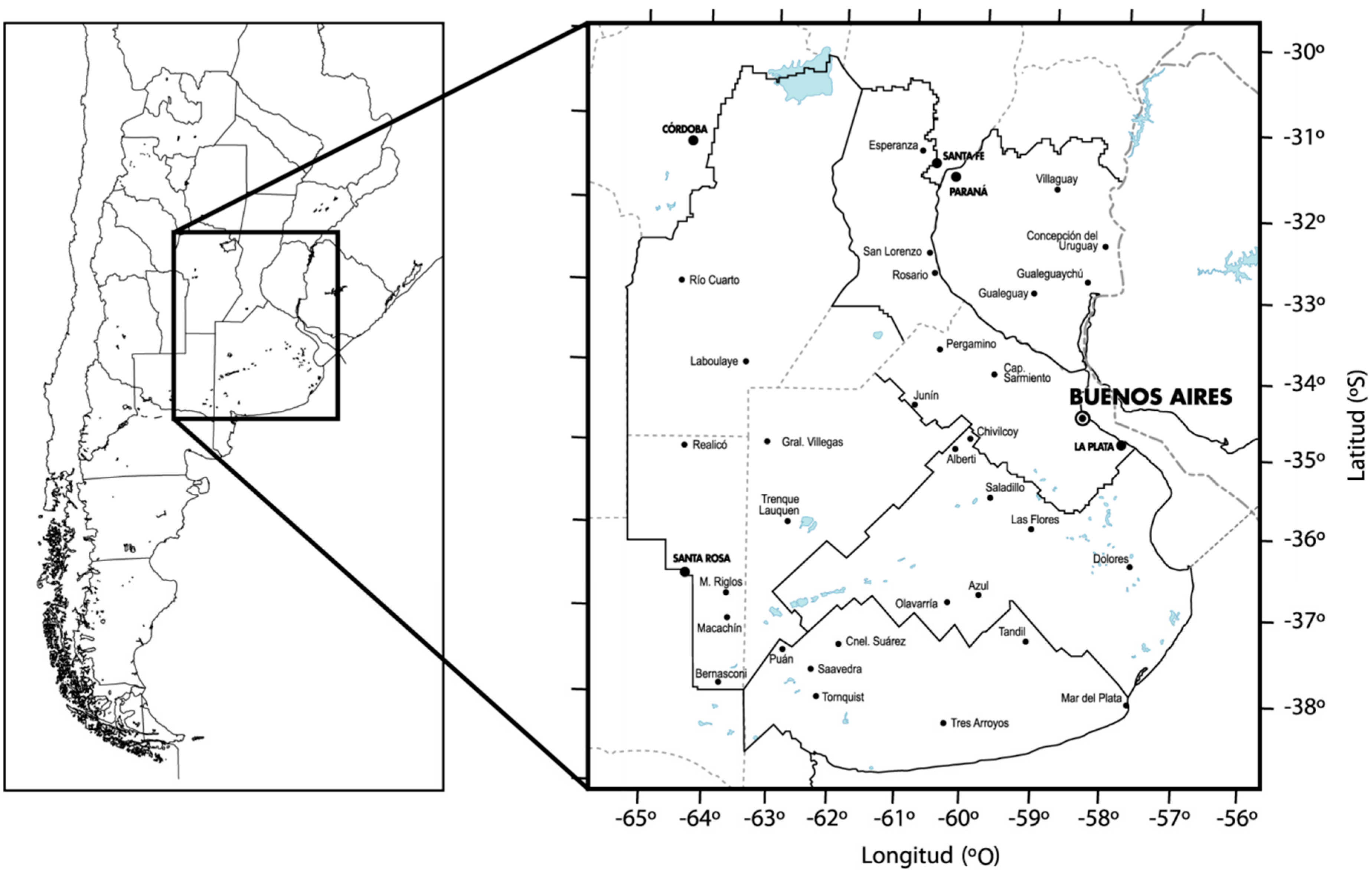
Annual rainfall data from 34 locations in the Pampa Region for the period 1941–2010 were used (Table 1, Figure 1). Seven of the locations belonged to the Southern Pampa, eight to the Central Pampa, seven to the Flooding Pampa, five to the Mesopotamian Pampa and seven to the Rolling Pampa. Data were provided by the National Weather Service (Servicio Meteorológico Nacional) and the National Institute for Agricultural Technology (INTA). Data for the Pacific Decadal Oscillation (PDO), the Atlantic Multidecadal Oscillation (AMO) and the Southern Oscillation Index (SOI) were obtained from the online database at: http://www.esrl.noaa.gov/psd/data/climateindices/list/.

Table 1. Position of the different locations in the Pampa Region.

Location	Latitude (S)	Longitude (W)	Altitude (msl)	Pampa Sub-Region
Esperanza	31°27′	60° 55′	38	Rolling
San Lorenzo	32°44′	60° 44′	40	Rolling
Rosario	32°57′	60° 39′	25	Rolling
Pergamino	33°44′	60° 36′	56	Rolling
Cap. Sarmiento	34°10′	59° 48′	54	Rolling
Junin	34°35′	60° 56′	81	Rolling
La Plata	34°55′	57° 57′	26	Rolling
Paraná	31°43′	60° 31′	77	Mesopotamian
Villaguay	31°52′	59° 00′	40	Mesopotamian
C del Uruguay	32°29′	58° 14′	50	Mesopotamian
Gualeguaychú	33°00′	58° 30′	15	Mesopotamian
Gualeguay	33°08′	59° 19′	12	Mesopotamian
Río Cuarto	33°07′	64° 20′	452	Central
Laboulaye	34°07′	63° 23′	131	Central
Gral. Villegas	35°01′	63° 00′	105	Central
Realicó	35°01′	64° 15′	146	Central
Trenque Lauquen	35°58′	62° 43′	80	Central
Riglos	36°51′	63° 42′	126	Central
Macachín	37°09′	63° 39′	130	Central
Bernasconi	37°54′	63° 43′	162	Central
Chivilcoy	34°53′	60° 01′	53	Flooding
Alberti	35°01′	60° 16′	38	Flooding
Saladillo	35°38′	59° 46′	43	Flooding
Las Flores	36°03′	59° 06′	36	Flooding
Dolores	36°18′	57° 40′	7	Flooding
Azul	36°46′	59° 51′	137	Flooding
Olavarría	36°53′	60° 19′	150	Flooding
Tandil	37°19′	59° 08′	188	Southern
Cnel.Suárez	37°28′	61° 56′	298	Southern
Puán	37°32′	62° 46′	222	Southern
Saavedra	37°45′	62° 21′	334	Southern
Mar del Plata	38°00′	57° 33′	38	Southern
Tornquist	38°06′	62° 14′	276	Southern
Tres Arroyos	38°22′	60° 16′	98	Southern

Table 1. Position of the different locations in the Pampa Region.

Location	Latitude (S)	Longitude (W)	Altitude (msl)	Pampa Sub-Region
Esperanza	31°27′	60° 55′	38	Rolling
San Lorenzo	32°44′	60° 44′	40	Rolling
Rosario	32°57′	60° 39′	25	Rolling
Pergamino	33°44′	60° 36′	56	Rolling
Cap. Sarmiento	34°10′	59° 48′	54	Rolling
Junin	34°35′	60° 56′	81	Rolling
La Plata	34°55′	57° 57′	26	Rolling
Paraná	31°43′	60° 31′	77	Mesopotamian
Villaguay	31°52′	59° 00′	40	Mesopotamian
C del Uruguay	32°29′	58° 14′	50	Mesopotamian
Gualeguaychú	33°00′	58° 30′	15	Mesopotamian
Gualeguay	33°08′	59° 19′	12	Mesopotamian
Río Cuarto	33°07′	64° 20′	452	Central
Laboulaye	34°07′	63° 23′	131	Central
Gral. Villegas	35°01′	63° 00′	105	Central
Realicó	35°01′	64° 15′	146	Central
Trenque Lauquen	35°58′	62° 43′	80	Central
Riglos	36°51′	63° 42′	126	Central
Macachín	37°09′	63° 39′	130	Central
Bernasconi	37°54′	63° 43′	162	Central
Chivilcoy	34°53′	60° 01′	53	Flooding
Alberti	35°01′	60° 16′	38	Flooding
Saladillo	35°38′	59° 46′	43	Flooding
Las Flores	36°03′	59° 06′	36	Flooding
Dolores	36°18′	57° 40′	7	Flooding
Azul	36°46′	59° 51′	137	Flooding
Olavarría	36°53′	60° 19′	150	Flooding
Tandil	37°19′	59° 08′	188	Southern
Cnel.Suárez	37°28′	61° 56′	298	Southern
Puán	37°32′	62° 46′	222	Southern
Saavedra	37°45′	62° 21′	334	Southern
Mar del Plata	38°00′	57° 33′	38	Southern
Tornquist	38°06′	62° 14′	276	Southern
Tres Arroyos	38°22′	60° 16′	98	Southern

Figure 1. Location map of the Pampa Region, sub regions and localities.

Figure 1. Location map of the Pampa Region, sub regions and localities.

2.1. Homogeneity Test

A series of climate data is uniform if “... variations have only been caused by variations in weather and climate” [24]. A climatic series may no longer be uniform if the measuring station has changed its location, instruments, or weather observation procedures [25].

According to the previous statement, pre-1941 data were discarded because, in the period 1932–1940, the Argentine National Weather Service, proceeded to change the A type rain gauges that were previously used, by the B type rain gauges [26].

The homogeneity of the precipitation series was tested using [27] Standard Normal Homogeneity Test (SNHT) on AnClim software [28]. The test was applied to series of annual values, using the average annual rainfall of each sub-region as a reference series.

For each series a series of ratios ${\left|q_i\right|}_{i=1}^N$ were estimated between the observed value of the series to which the test was applied and the value of the reference series. The standardized series of ratios ${\left|z_i\right|}_{i=1}^N$ were estimated for which

$$z_i = (q_i-\overline{q_i} )/\text{Sq}$$

(1)

where $\overline{q}$ and sq are the mean and sample standard deviation of the qi series.

Let 1 ≤ ν < N and μ1 ≠ μ2 where N is the number of years of data available.

The purpose is to test the null hypothesis: $H_0:z_i~N\left(0,1\right) \forall i$

With respect to the alternative hypothesis:

$$\begin{gathered} H_1:z_i~N\left({\mu }_1,1\right)i\le v \\ {H}_1:z_i~N\left({\mu }_2,1\right)i>v \end{gathered}$$

The null hypothesis implies that the mean of standardized series z_i does not change over time, whereas the alternative hypothesis suggests that for some time ν there is a change in the mean of the series.

The test statistic to determine whether a change has occurred in the mean of series z_i is

$$T_0=\underset{1\le v<N}{\text{max}}\left\{T_v\right\}$$

(2)

where

$$\text{Tν} = \text{ν}{\overline{\text{z}}}_1^2+\left(\text{N}-\text{ν}\right){\overline{\text{z}}}_2^2$$

(3)

${\overline{\text{z}}}_1$ and ${\overline{\text{z}}}_2$ are the sample means of the first ν and last (N − ν) values of the series z_i. If T₀ is greater than some critical level for a given significance level of the test, the null hypothesis which states that the series is homogenous can be rejected. According to [29], the critical values for the test at significance level α = 0.05 for a series length N = 70 is 8.800. To adjust the detected inhomogeneities, the setting method indicated in [30] was applied using the software AnClim [28].

The average series was calculated for the homogeneous and the adjusted inhomogeneous annual precipitation series of each sub region which, in turn, was used to evaluate shifts in the mean value.

2.2. Detecting Shifts in the Mean

Shifts in mean annual precipitation were detected using Hubert’s method of segmentation of hydrometeorological time series [31]. The precipitation time series for each sub region was calculated as the mean of the corresponding homogeneous series, as defined by the SNHT test.

Hubert’s segmentation method divides the series into m segments (m > 1) so that the calculated mean over the entire series is significantly different from the means of neighboring segments.

Segmentation is defined as follows: Any series x_i, i = i₁, i₂ with i₁ ≥ 1 and i₂ ≤ N where (i₁ < i₂) is a segment of the initial series of (x_i), I = 1, ..., N.

Any division of the initial series into m segments is an m-order segmentation of this series. Thus, from a particular m order segmentation performed on the initial series, we define:

$$\begin{gathered} i_k,k = 1,2,\dots , m \\ {n}_k = i_k - i_{k - 1} \end{gathered}$$

$${\overline{x}}_k= \left[{\displaystyle \sum }_{i=i_{k-1}+1}^{i=i_k}{x}_i\right]/n_k$$

(4)

$$D_m= {\displaystyle \sum }_{k=1}^{k=m}{d}_k$$

(5)

with

$$d_k= {\displaystyle \sum }_{i=i_{k-1}+1}^{i=i_k}{\left(x_i-{\overline{x}}_k\right)}^2$$

(6)

The segmentation obtained should be such that for a given segment order m, the standard deviation D_m is minimal. This is a necessary but not a sufficient condition to determine the optimal segmentation. It should be noted that the means of two adjacent segments must be significantly different. This constraint is met by applying the Scheffé test [32].

The variability coefficient was calculated using the standard deviation and the mean of each respective segment.

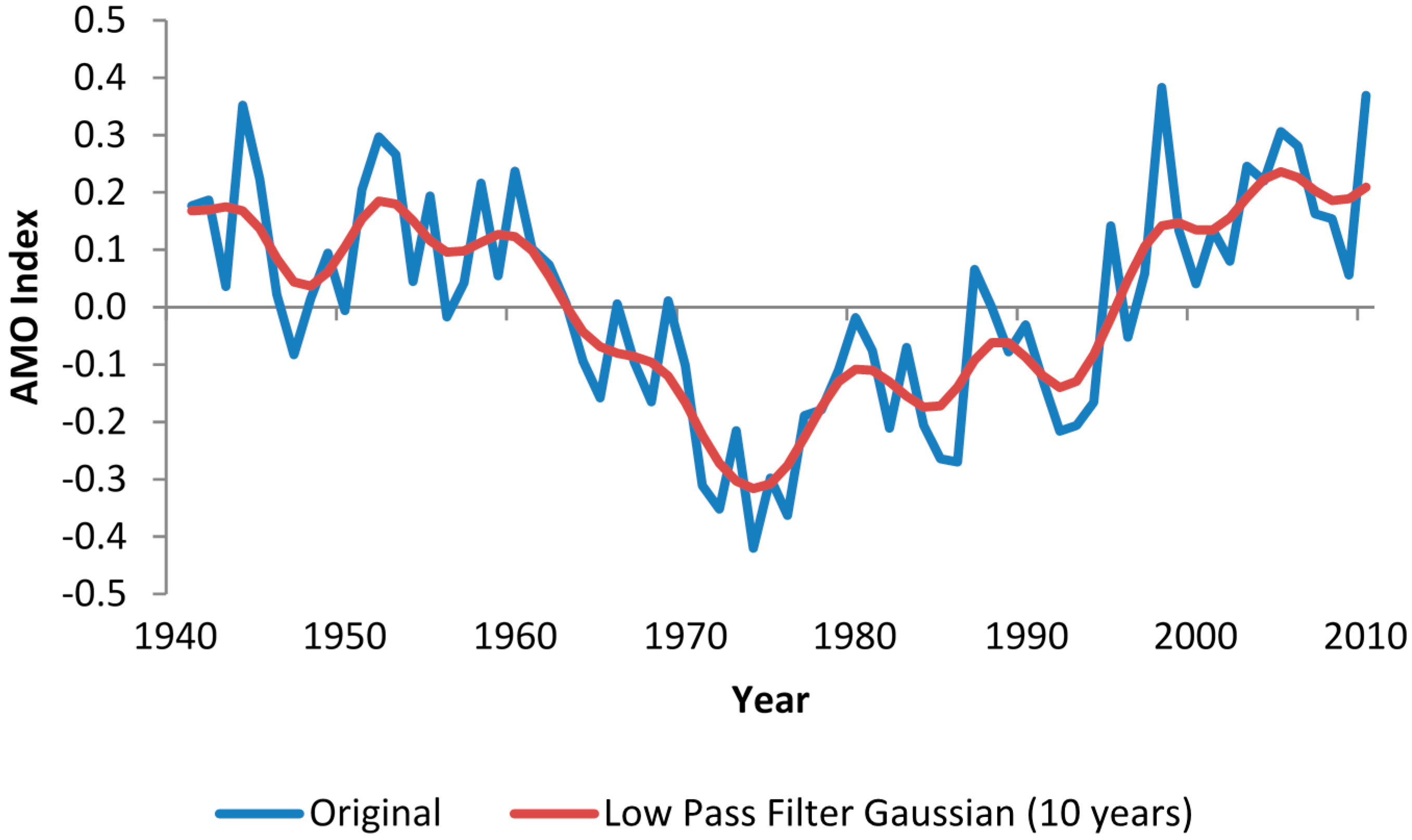
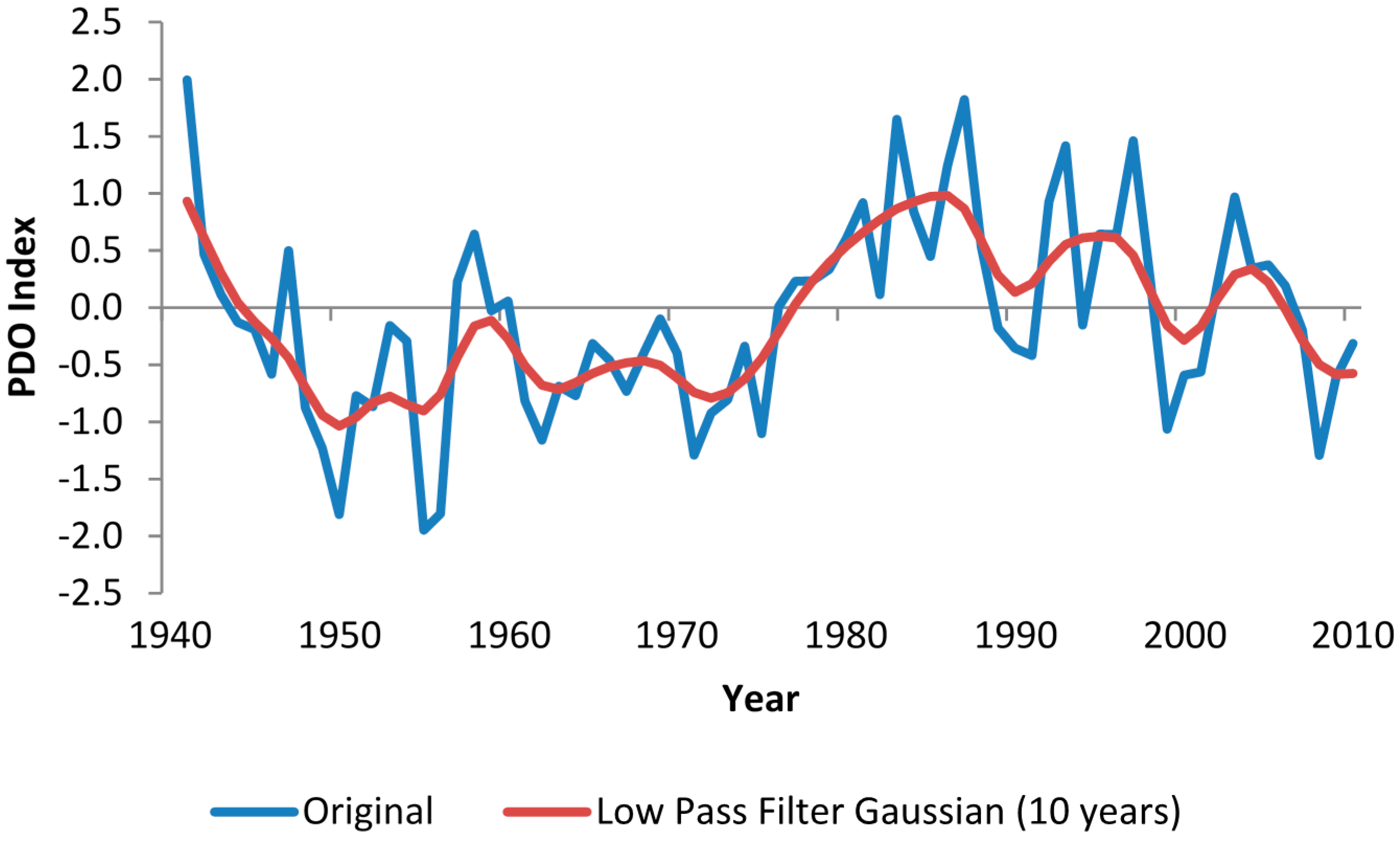
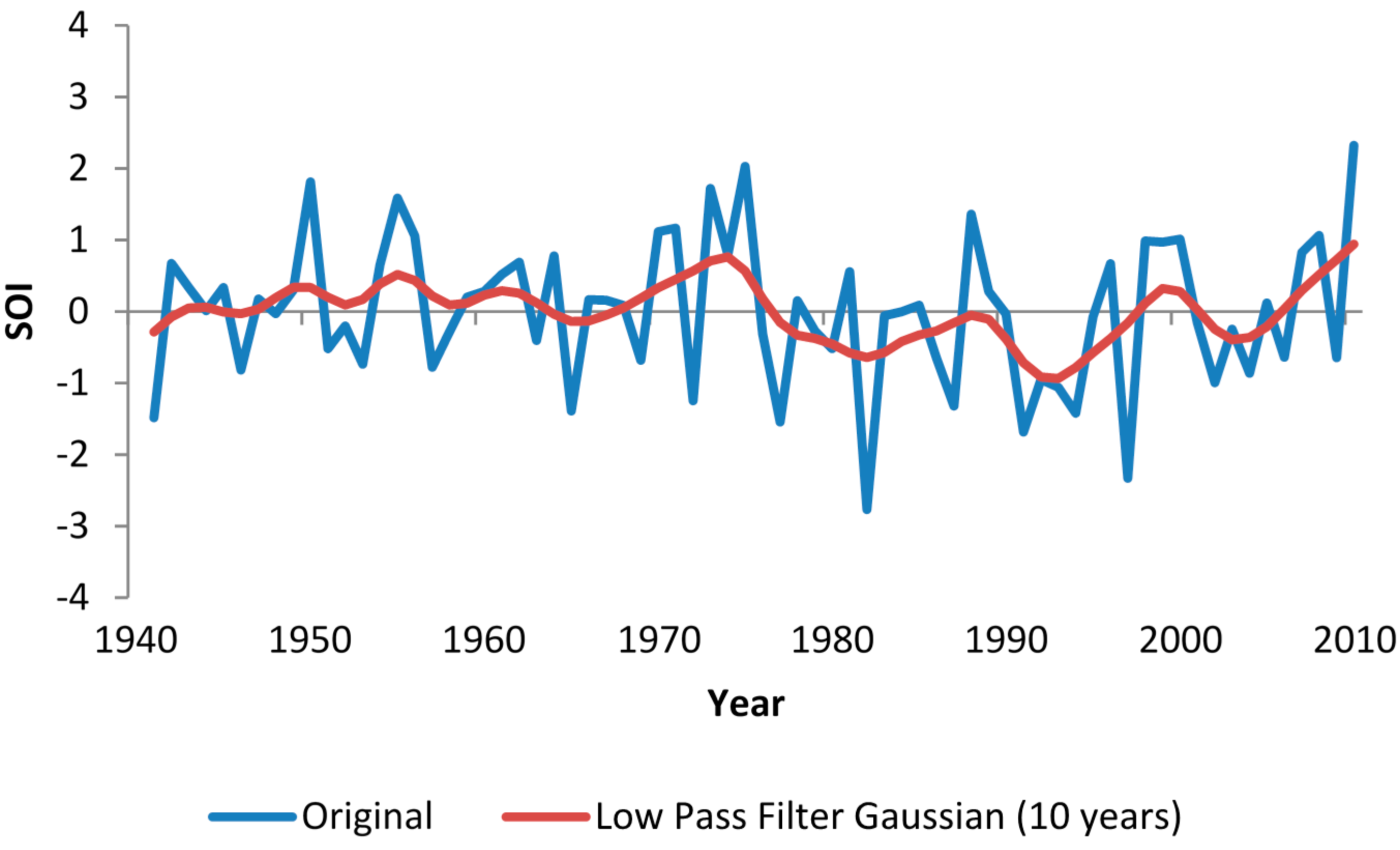
2.3.The AMO-PDO-SOI-precipitation relationship

Teleconnections from AMO, PDO and SOI to annual rainfall were evaluated through Pearson correlation analysis. Since [33] consider that PDO events persist for over 20 years, correlation lags were performed from 1 to 20 years.

The AMO and PDO are ocean oscillations with negative and positive phases taking between 20 and 40 years [34,35,36,37], thus given total cycles of about 40 to 80 years (Figure 2 and Figure 3). Consequently, they can be associated with low frequency changes in rainfall. On the other hand, the SOI is an atmospheric index with an annual oscillation period [38] and is therefore associated with high frequency variations in rainfall (Figure 4).

Figure 2. Atlantic Multidecadal Oscillation (AMO).

Figure 2. Atlantic Multidecadal Oscillation (AMO).

Figure 3. Pacific Multidecadal Oscillation (PDO).

Figure 3. Pacific Multidecadal Oscillation (PDO).

Figure 4. Southern Oscillation Index (SOI).

Figure 4. Southern Oscillation Index (SOI).

3. Results and Discussion

3.1. Homogeneity Test

Twenty-six of the available annual rainfall series (Table 2) showed a T value smaller than the critical value [29] and can be considered homogeneous at the level of significance α = 0.05. The other eight series had T values greater than the critical value and were thus considered non-homogeneous. They were adjusted for the analysis by the setting method indicated in [30].

Table 2. Test results of the Standard Normal Homogeneity Test (SNHT) applied to annual precipitation series from the Pampa Region. (* indicates that the T value exceeds 95%).

Location	Shift Year	T Value		Shift Year Adjusted	T Value Adjusted
Esperanza	1944	4.315
San Lorenzo	2003	3.356
Rosario	1973	13.954	*	1996	7.493
Pergamino	2005	6.993
Cap. Sarmiento	1952	24.639	*	1996	5.321
Junin	2001	3.305
La Plata	2008	7.669
Paraná	1948	5.299
Villaguay	1943	6.498
C del Uruguay	1995	5.444
Gualeguaychú	1979	3.302
Gualeguay	1975	8.022
Río Cuarto	1968	22.476	*	1985	3.796
Laboulaye	1976	5.436
Gral. Villegas	2003	5.370
Realicó	2010	6.746
Trenque Lauquen	1956	7.366
Riglos	1977	10.936	*	1946	3.084
Macachín	2009	3.678
Bernasconi	2005	5.645
Chivilcoy	1990	15.885	*	1999	6.327
Alberti	2000	2.906
Saladillo	1977	3.186
Las Flores	1990	2.312
Dolores	2001	5.103
Azul	1991	6.187
Olavarría	1944	4.596
Tandil	1982	5.874
Cnel. Suárez	2005	9.750	*	2009	2.843
Puán	1976	2.431
Saavedra	1958	9.530	*	2009	4.720
Mar del Plata	2000	3.226
Tornquist	1964	3.887
Tres Arroyos	2010	10.071	*	1963	2.905

Table 2. Test results of the Standard Normal Homogeneity Test (SNHT) applied to annual precipitation series from the Pampa Region. (* indicates that the T value exceeds 95%).

Location	Shift Year	T Value		Shift Year Adjusted	T Value Adjusted
Esperanza	1944	4.315
San Lorenzo	2003	3.356
Rosario	1973	13.954	*	1996	7.493
Pergamino	2005	6.993
Cap. Sarmiento	1952	24.639	*	1996	5.321
Junin	2001	3.305
La Plata	2008	7.669
Paraná	1948	5.299
Villaguay	1943	6.498
C del Uruguay	1995	5.444
Gualeguaychú	1979	3.302
Gualeguay	1975	8.022
Río Cuarto	1968	22.476	*	1985	3.796
Laboulaye	1976	5.436
Gral. Villegas	2003	5.370
Realicó	2010	6.746
Trenque Lauquen	1956	7.366
Riglos	1977	10.936	*	1946	3.084
Macachín	2009	3.678
Bernasconi	2005	5.645
Chivilcoy	1990	15.885	*	1999	6.327
Alberti	2000	2.906
Saladillo	1977	3.186
Las Flores	1990	2.312
Dolores	2001	5.103
Azul	1991	6.187
Olavarría	1944	4.596
Tandil	1982	5.874
Cnel. Suárez	2005	9.750	*	2009	2.843
Puán	1976	2.431
Saavedra	1958	9.530	*	2009	4.720
Mar del Plata	2000	3.226
Tornquist	1964	3.887
Tres Arroyos	2010	10.071	*	1963	2.905

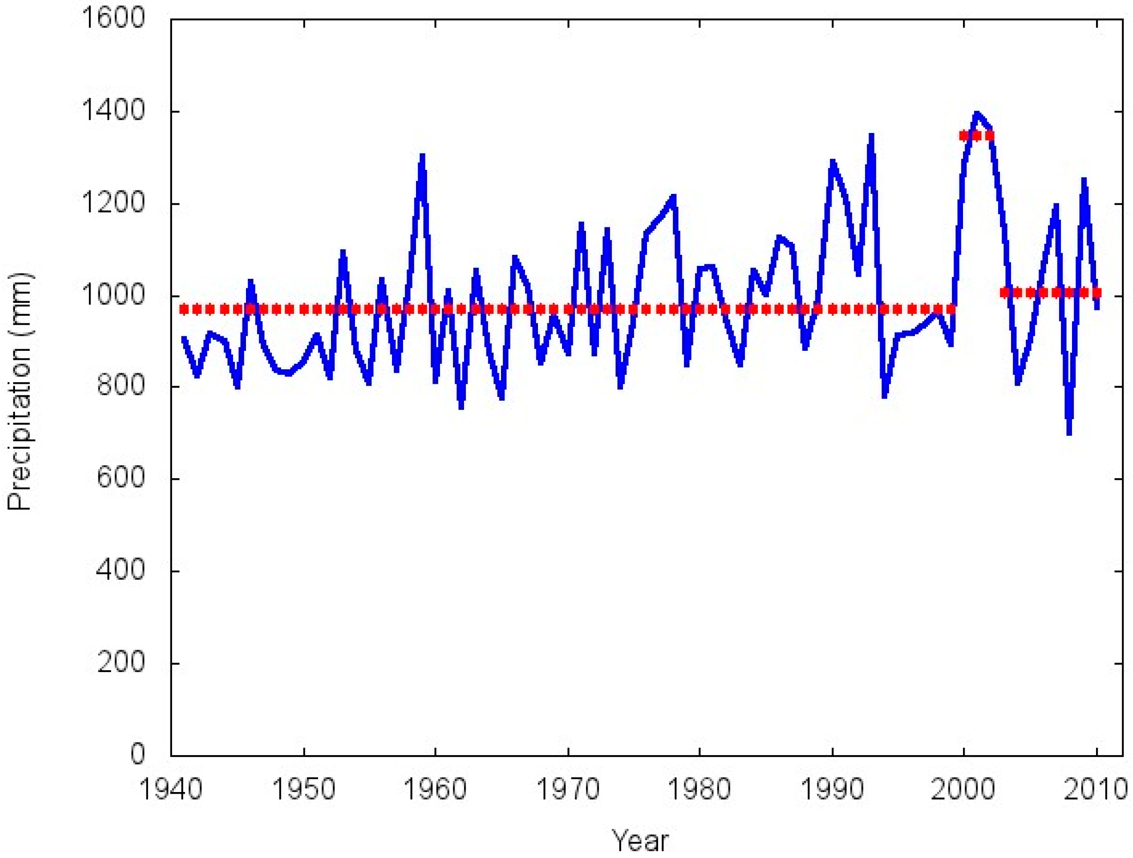
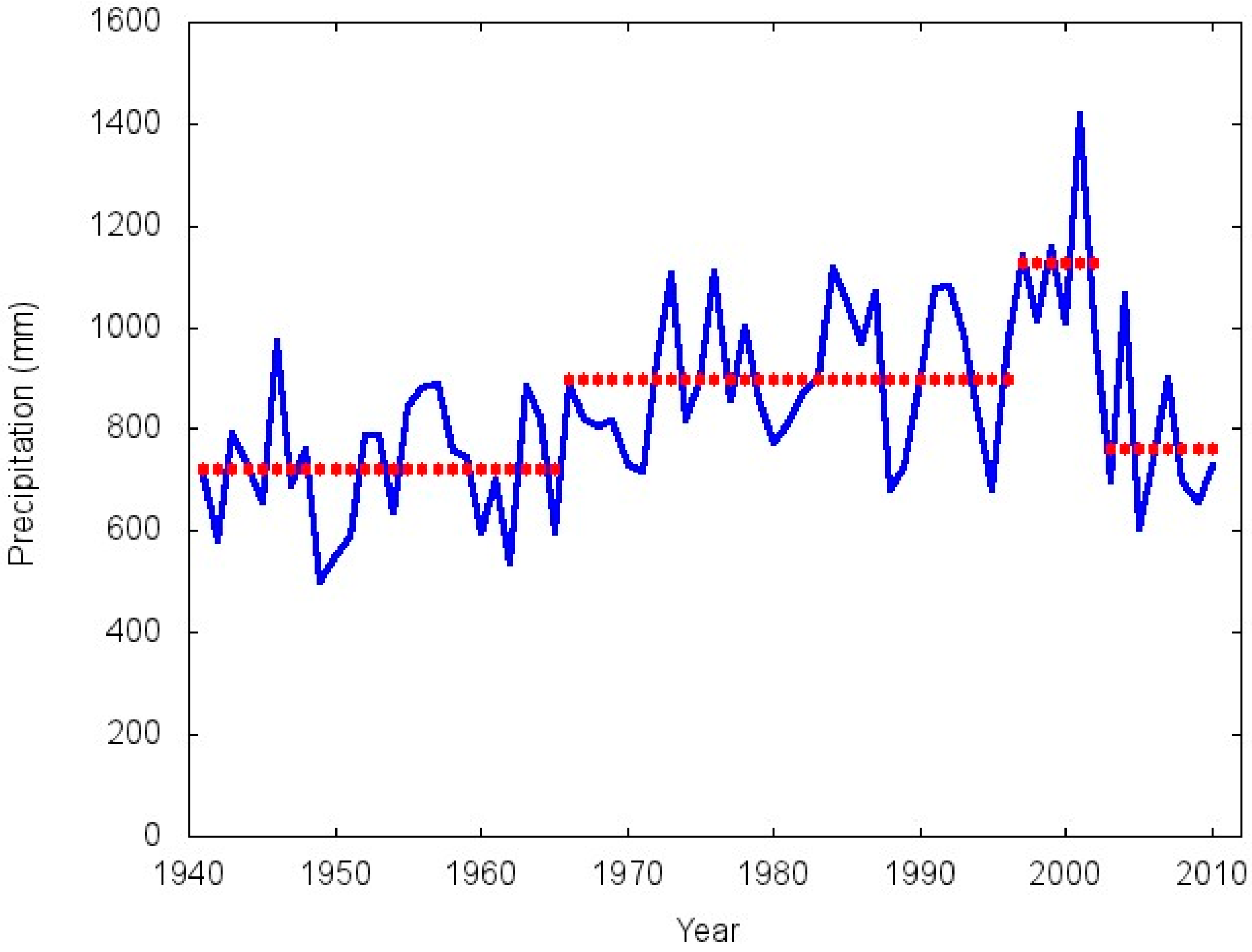
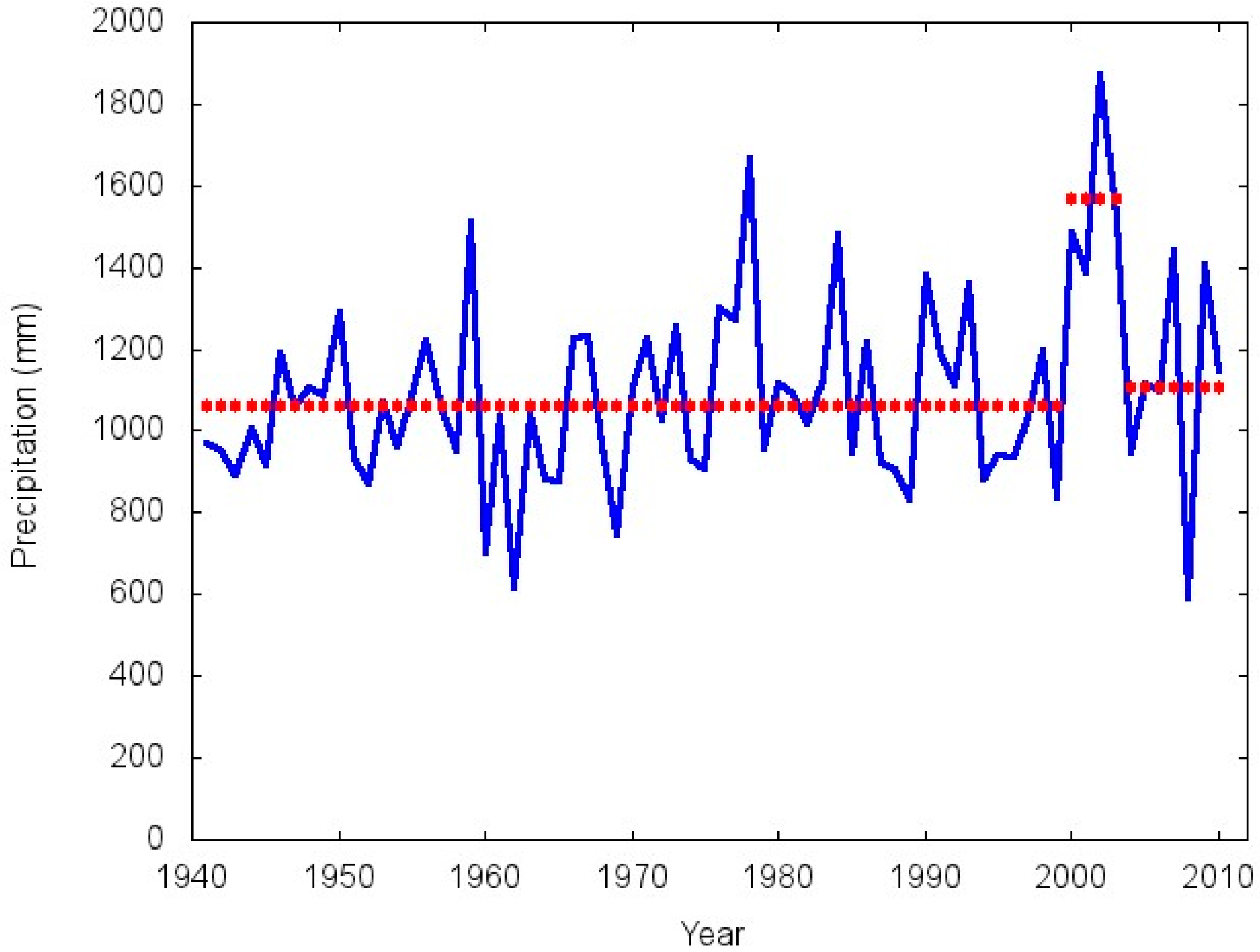
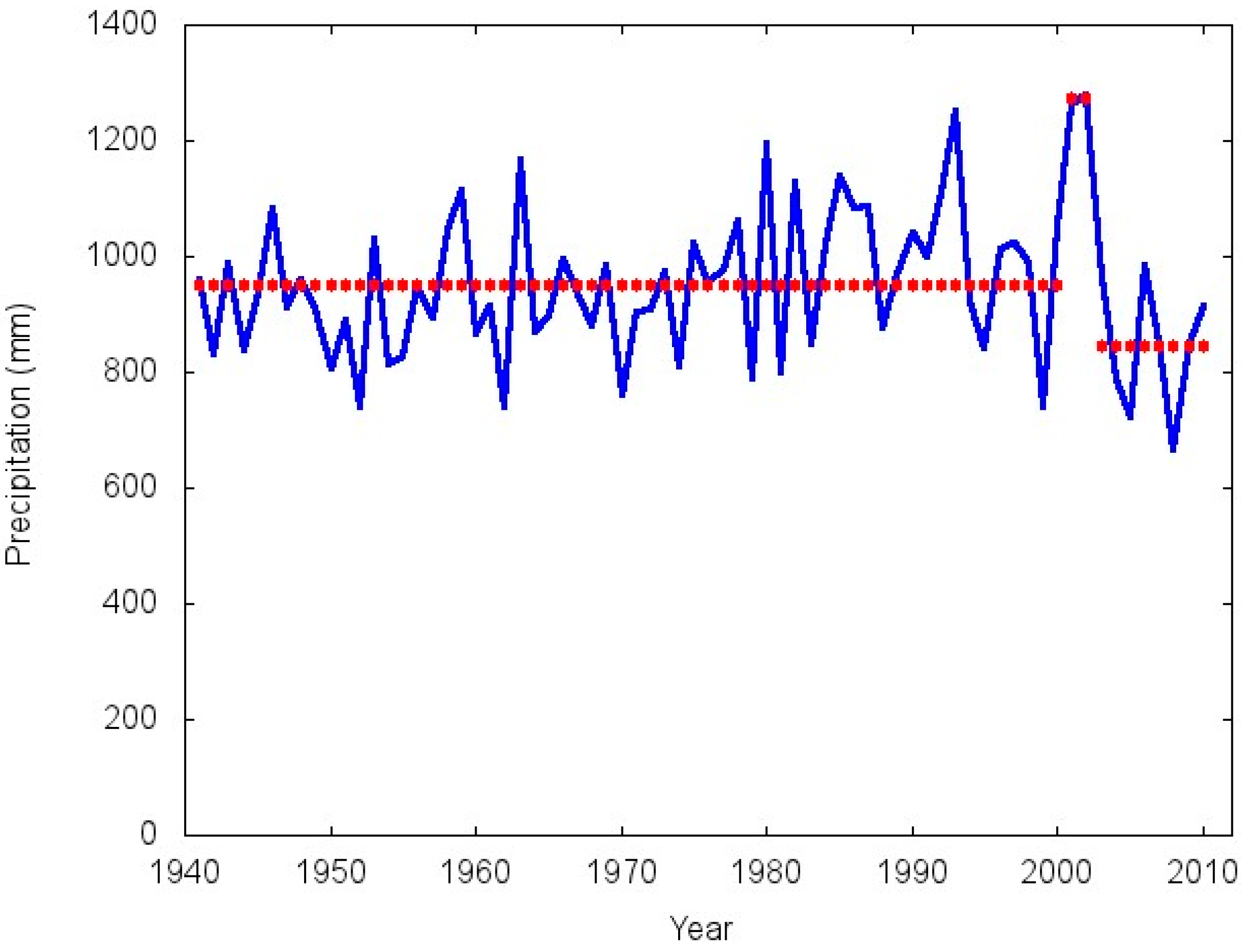
3.2. Detecting Changes in the Mean

The results for the sub-regional average annual rainfall series of the Argentine Pampas Region by Hubert’s segmentation method [31] are detailed in Table 3.

Table 3. Segmentation of the annual precipitation series for the sub-regions of the Pampa Region by Hubert’s segmentation method [31].

Sub-Regions	Sub-Period	Mean (mm)	Standard Deviation	Variation Coefficient
Rolling Pampa	1941–1999	971.9	142.8	14.7
	2000–2002	1349.3	56.7	4.2
	2003–2010	1005.2	191.8	19.0
Mesopotamian Pampa	1941–1999	1062.9	197.9	18.6
	2000–2003	1568.9	211.1	13.4
	2004–2010	1108.0	289.5	26.1
Central Pampa	1941–1965	721.3	126.2	17.5
	1966–1996	900.0	132.8	14.7
	1997–2002	1126.0	158.8	14.1
	2003–2010	762.2	149.9	19.7
Flooding Pampa	1941–2000	952.7	118.9	12.5
	2001–2002	1272.2	10.9	0.9
	2003–2010	844.5	112.9	13.4
Southern Pampa	1941–2000	819.3	137.1	16.7
	2001–2002	1155.2	85.9	7.4
	2003–2010	745.3	103.5	13.9

Table 3. Segmentation of the annual precipitation series for the sub-regions of the Pampa Region by Hubert’s segmentation method [31].

Sub-Regions	Sub-Period	Mean (mm)	Standard Deviation	Variation Coefficient
Rolling Pampa	1941–1999	971.9	142.8	14.7
	2000–2002	1349.3	56.7	4.2
	2003–2010	1005.2	191.8	19.0
Mesopotamian Pampa	1941–1999	1062.9	197.9	18.6
	2000–2003	1568.9	211.1	13.4
	2004–2010	1108.0	289.5	26.1
Central Pampa	1941–1965	721.3	126.2	17.5
	1966–1996	900.0	132.8	14.7
	1997–2002	1126.0	158.8	14.1
	2003–2010	762.2	149.9	19.7
Flooding Pampa	1941–2000	952.7	118.9	12.5
	2001–2002	1272.2	10.9	0.9
	2003–2010	844.5	112.9	13.4
Southern Pampa	1941–2000	819.3	137.1	16.7
	2001–2002	1155.2	85.9	7.4
	2003–2010	745.3	103.5	13.9

The Rolling Pampa sub-region average (Figure 5) showed two abrupt changes. The first of these was positive, with the average annual precipitation rising from 971.9 mm during 1941–1999 the sub-period, to 1349.3 mm during a very short sub-period ranging from 2000 to 2002. In 2003, a negative change dropped the average annual rainfall to 1005.2 mm, only slightly higher than what it had been in the initial 1941–1999 sub-period.

Figure 5. Annual precipitation and means for sub-periods in the Rolling Pampa sub-region by Hubert’s segmentation method.

Figure 5. Annual precipitation and means for sub-periods in the Rolling Pampa sub-region by Hubert’s segmentation method.

The mean for the Mesopotamian Pampa sub-region showed a very similar behavior with two abrupt shifts (Figure 6). The first of these was positive, with annual average rainfall increasing from 1062.9 mm during the 1941–1999 sub-period to 1568.9 mm during a short sub-period between 2000 and 2003. The second abrupt change, which began in 2004, was negative, with average annual rainfall dropping to 1108.0 mm, only slightly higher than what it had been in the initial 1941–1999 sub-period.

Figure 6. Annual precipitation and means for sub-periods in the Mesopotamian Pampa sub region by Hubert’s segmentation method.

Figure 6. Annual precipitation and means for sub-periods in the Mesopotamian Pampa sub region by Hubert’s segmentation method.

The Central Pampa sub region (Figure 7) showed a more complex behavior, with two abrupt positive changes in close succession. The first brought average annual precipitation from 721.3 mm during the sub-period 1941–1965, to 900.0 mm during the sub-period 1966–1996. The second abrupt positive change raised average annual rainfall to 1126.0 mm between 1997 and 2002. It is noteworthy that after this short wet sub-period of just five years, a negative abrupt change beginning in 2003 reduced average annual rainfall to 762.2 mm, very similar to the mean precipitation for the initial 1941–1965 sub-period.

Figure 7. Annual precipitation and means for sub-periods in the Central Pampa sub region by Hubert’s segmentation method.

Figure 7. Annual precipitation and means for sub-periods in the Central Pampa sub region by Hubert’s segmentation method.

Figure 8. Annual precipitation and means for the 1941–2010 period in the Flooding Pampa sub-region.

Figure 8. Annual precipitation and means for the 1941–2010 period in the Flooding Pampa sub-region.

The mean for the Flooding Pampa sub-region showed two abrupt changes (Figure 8). The first was positive, with annual average rainfall increasing from 952.7 mm during the 1941–2000 sub-period, to 1272.2 mm for the 2001–2002 sub-period. The second abrupt change, which began in 2003, was negative, with average annual rainfall dropping to 844.5 mm, which is lower than it had been during the initial 1941–2000 sub-period.

The mean for the Southern Pampa sub-region showed two abrupt changes (Figure 9). The first was positive, with annual average rainfall increasing from 819.3 mm during the 1941–2000 sub-period, to 1155.2 mm for the 2001–2002 sub-period. The second abrupt change, which began in 2003, was negative. Here average annual rainfall dropped to 745.3 mm, which is lower than it had been during the initial 1941–2000 sub-period.

Figure 9. Annual precipitation and means for the sub-periods in the Southern Pampa sub region by Hubert’s segmentation method.

Figure 9. Annual precipitation and means for the sub-periods in the Southern Pampa sub region by Hubert’s segmentation method.

3.3. Associations from Rainfall to the AMO, PDO and SOI

The most significant AMO teleconnections to precipitation in Argentina’s Pampa Region were observed at lag −10 years in the Rolling (RP), Mesopotamian (MP), Flooding (FP) and Southern (SP) sub-regions and at lag −8 years in the Central Pampa sub-region (Table 4).

The fact that these correlations are negative indicates that, when the Atlantic Ocean warms, rainfall tends to show a decrease in mean value and an increase in variability over much of the Pampa Region. This has a negative impact on agricultural production.

The fact that AMO significant correlations begin as much as lag −10, suggest that its influence is transferred very slowly to the atmosphere, and therefore it takes several years before sensible changes in rainfall behavior are detected.

It also suggest that AMO influence may be cumulative, requiring several years to reach an activation threshold strong enough to cause changes in rainfall behavior.

This also causes that, in spite that AMO is mainly a summer signal, it is capable of influencing annual values.

Statistically significant PDO teleconnections to precipitation in Argentina’s Pampa Region were observed at lags of 4 years in the Central Pampa sub-region, and at lags of 4 to 6 years in the Flooding and Southern Pampa sub-regions (Table 5).

Table 4. Correlation coefficients between the Atlantic Multidecadal Oscillation (AMO) and annual rainfall time series for the Pampa Region.

Lag	RP	MP	CP	FP	SP
−20	−0.0234	−0.0295	−0.1298	−0.0865	−0.0985
−19	−0.1980	−0.1183	−0.2139	−0.1938	−0.1513
−18	−0.1817	−0.0829	−0.2486	−0.2476	−0.2433
−17	−0.3121	−0.1666	−0.3049	−0.2739	−0.2880
−16	−0.3537	−0.2378	−0.3474	−0.2631	−0.2292
−15	−0.2213	0.0011	−0.3032	−0.1528	−0.1696
−14	−0.1662	−0.0323	−0.2564	−0.0857	−0.1255
−13	−0.2599	−0.0959	−0.3388	−0.2031	−0.2153
−12	−0.1894	−0.0677	−0.3549	−0.2341	−0.2339
−11	−0.1803	−0.1188	−0.4051	−0.2725	−0.2863
−10	−0.3154	−0.2784	−0.4779	−0.3924	−0.4367
−9	−0.2784	−0.2620	−0.4186	−0.3249	−0.3048
−8	−0.2263	−0.1892	−0.5283	−0.3139	−0.4121
−7	−0.2617	−0.1803	−0.5054	−0.2564	−0.3619
−6	−0.1967	−0.1124	−0.3399	−0.2136	−0.2970
−5	−0.1884	−0.0405	−0.4449	−0.1158	−0.2295
−4	−0.1047	0.0457	−0.2532	−0.1703	−0.1450
−3	−0.0188	0.0391	−0.1540	−0.0716	−0.0566
−2	−0.0887	−0.0878	−0.2529	−0.1607	−0.0947
−1	−0.0956	−0.0383	−0.2681	−0.2482	−0.2158
0	−0.1376	−0.1107	−0.3000	−0.2237	−0.2291

RP Rolling Pampa, MP Mesopotamian Pampa, CP Central Pampa, FP Flooding Pampa, SP Southern Pampa; The critical value of Pearson’s correlation coefficient at the 0.05 level of significance is 0.232. Values in bold are statistically significant at the 95% level.

Table 4. Correlation coefficients between the Atlantic Multidecadal Oscillation (AMO) and annual rainfall time series for the Pampa Region.

Lag	RP	MP	CP	FP	SP
−20	−0.0234	−0.0295	−0.1298	−0.0865	−0.0985
−19	−0.1980	−0.1183	−0.2139	−0.1938	−0.1513
−18	−0.1817	−0.0829	−0.2486	−0.2476	−0.2433
−17	−0.3121	−0.1666	−0.3049	−0.2739	−0.2880
−16	−0.3537	−0.2378	−0.3474	−0.2631	−0.2292
−15	−0.2213	0.0011	−0.3032	−0.1528	−0.1696
−14	−0.1662	−0.0323	−0.2564	−0.0857	−0.1255
−13	−0.2599	−0.0959	−0.3388	−0.2031	−0.2153
−12	−0.1894	−0.0677	−0.3549	−0.2341	−0.2339
−11	−0.1803	−0.1188	−0.4051	−0.2725	−0.2863
−10	−0.3154	−0.2784	−0.4779	−0.3924	−0.4367
−9	−0.2784	−0.2620	−0.4186	−0.3249	−0.3048
−8	−0.2263	−0.1892	−0.5283	−0.3139	−0.4121
−7	−0.2617	−0.1803	−0.5054	−0.2564	−0.3619
−6	−0.1967	−0.1124	−0.3399	−0.2136	−0.2970
−5	−0.1884	−0.0405	−0.4449	−0.1158	−0.2295
−4	−0.1047	0.0457	−0.2532	−0.1703	−0.1450
−3	−0.0188	0.0391	−0.1540	−0.0716	−0.0566
−2	−0.0887	−0.0878	−0.2529	−0.1607	−0.0947
−1	−0.0956	−0.0383	−0.2681	−0.2482	−0.2158
0	−0.1376	−0.1107	−0.3000	−0.2237	−0.2291

RP Rolling Pampa, MP Mesopotamian Pampa, CP Central Pampa, FP Flooding Pampa, SP Southern Pampa; The critical value of Pearson’s correlation coefficient at the 0.05 level of significance is 0.232. Values in bold are statistically significant at the 95% level.

The fact that the correlations are positive indicates that as the North Pacific warms, precipitation increases in part of the Pampa Region and vice versa. Therefore, positive phases of this cycle favor the Argentine agricultural sector, while the negative phases are unfavorable.

As in the case of AMO, the fact that significant correlations begin as much as lag −10, suggest that its influence is transferred very slowly to the atmosphere, and therefore it takes several years before sensible changes in rainfall behavior are detected.

Similarly, PDO influence may be cumulative, requiring several years to reach an activation threshold strong enough to cause changes in rainfall behavior.

Although significant, all PDO correlations were weaker than those of AMO, showing that, by itself, It has little influence on the pampean rainfall regime. Nevertheless it may have some synergetic interaction with the AMO, whose cycle is almost inverse.

Statistically significant SOI teleconnections to precipitation in the Argentina Pampa Region were observed during the first year of each period in the Flooding and Southern Pampa sub-regions and at lag 7 years in the Central Pampa sub-region (Table 6).

Table 5. Correlation coefficients between the Pacific Decadal Oscillation (PDO) and the annual rainfall time series for the Pampa Region.

Lag	RP	MP	CP	FP	SP
−20	−0.0543	0.0568	−0.1610	−0.0764	−0.0577
−19	0.0604	0.2292	−0.1320	−0.0274	−0.0830
−18	0.0036	0.0694	−0.0706	−0.0665	−0.0220
−17	−0.0109	−0.0062	−0.0415	0.0065	0.0634
−16	−0.0577	0.0683	0.0108	−0.0543	0.0128
−15	−0.0162	0.1001	0.0764	0.0620	0.0741
−14	0.0008	0.1935	0.0422	−0.0051	−0.0054
−13	0.0029	0.0735	−0.0938	−0.1100	−0.0600
−12	−0.0055	0.0036	−0.0171	−0.0738	0.0647
−11	−0.2090	−0.1962	−0.0649	−0.1414	−0.0270
−10	0.0132	0.1259	0.0272	0.0514	0.0792
−9	0.0106	0.0590	0.0504	0.1032	0.0867
−8	0.0225	0.0808	−0.0227	−0.0027	0.0134
−7	0.0333	0.0667	0.0253	0.0142	0.0136
−6	0.1821	0.1085	0.1702	0.3433	0.3007
−5	0.1672	0.1228	0.1776	0.3301	0.2436
−4	0.1207	−0.0415	0.3078	0.2349	0.2802
−3	0.0286	−0.0770	0.1123	0.0310	0.0494
−2	−0.1187	−0.1685	−0.0357	−0.0684	−0.1233
−1	−0.0206	−0.0640	0.0991	0.1014	0.0436
0	0.1565	0.0601	0.2094	0.2731	0.1721

RP Rolling Pampa, MP Mesopotamian Pampa, CP Central Pampa, FP Flooding Pampa, SP Southern Pampa; The critical value of Pearson’s correlation coefficient at the 0.05 level of significance is 0.232. Values in bold are statistically significant at the 95% level.

Table 5. Correlation coefficients between the Pacific Decadal Oscillation (PDO) and the annual rainfall time series for the Pampa Region.

Lag	RP	MP	CP	FP	SP
−20	−0.0543	0.0568	−0.1610	−0.0764	−0.0577
−19	0.0604	0.2292	−0.1320	−0.0274	−0.0830
−18	0.0036	0.0694	−0.0706	−0.0665	−0.0220
−17	−0.0109	−0.0062	−0.0415	0.0065	0.0634
−16	−0.0577	0.0683	0.0108	−0.0543	0.0128
−15	−0.0162	0.1001	0.0764	0.0620	0.0741
−14	0.0008	0.1935	0.0422	−0.0051	−0.0054
−13	0.0029	0.0735	−0.0938	−0.1100	−0.0600
−12	−0.0055	0.0036	−0.0171	−0.0738	0.0647
−11	−0.2090	−0.1962	−0.0649	−0.1414	−0.0270
−10	0.0132	0.1259	0.0272	0.0514	0.0792
−9	0.0106	0.0590	0.0504	0.1032	0.0867
−8	0.0225	0.0808	−0.0227	−0.0027	0.0134
−7	0.0333	0.0667	0.0253	0.0142	0.0136
−6	0.1821	0.1085	0.1702	0.3433	0.3007
−5	0.1672	0.1228	0.1776	0.3301	0.2436
−4	0.1207	−0.0415	0.3078	0.2349	0.2802
−3	0.0286	−0.0770	0.1123	0.0310	0.0494
−2	−0.1187	−0.1685	−0.0357	−0.0684	−0.1233
−1	−0.0206	−0.0640	0.0991	0.1014	0.0436
0	0.1565	0.0601	0.2094	0.2731	0.1721

RP Rolling Pampa, MP Mesopotamian Pampa, CP Central Pampa, FP Flooding Pampa, SP Southern Pampa; The critical value of Pearson’s correlation coefficient at the 0.05 level of significance is 0.232. Values in bold are statistically significant at the 95% level.

The fact that the correlations are negative indicates that when the trade winds strengthen, precipitation decreases in part of the Pampa Region and, conversely, when the trade winds slacken, precipitation increases. Therefore, the negative half of the SOI cycle, associated with “El Nino” events, favors the Argentine agricultural sector while the positive half, associated with “La Niña” events, is unfavorable.

It must be pointed out that SOI correlations to annual rainfall are necessarily weak because this atmospheric index acts predominantly during the spring and summer [39], and therefore its influence is blurred by the use of annual data.

Table 6. Correlation coefficients between the Southern Oscillation Index (SOI) and annual rainfall time series for the Pampa Region.

Lag	RP	MP	CP	FP	SP
−20	−0.1412	−0.1968	−0.1222	−0.1595	−0.1755
−19	−0.1681	−0.1501	−0.0653	−0.0865	−0.0105
−18	−0.0929	−0.1157	0.0724	0.0818	0.1036
−17	0.1892	0.2180	0.0089	0.1039	0.0454
−16	0.0157	−0.0846	0.0048	0.0524	0.0439
−15	−0.0841	−0.1398	−0.2318	−0.0977	−0.1329
−14	−0.0134	−0.0185	−0.0278	0.1175	0.0237
−13	−0.0938	−0.1056	0.0423	0.1033	0.0166
−12	−0.0162	0.0007	0.0804	0.1292	0.0089
−11	0.0608	0.0579	0.0197	0.0456	0.0087
−10	−0.2102	−0.1870	−0.2033	−0.1881	−0.1416
−9	−0.1095	−0.0979	−0.0246	−0.0499	−0.0109
−8	−0.2023	−0.2033	−0.0182	−0.1213	−0.0179
−7	−0.0267	−0.0123	−0.2904	−0.0061	−0.1194
−6	−0.1305	−0.1348	−0.1356	−0.1974	−0.1360
−5	−0.0313	0.0223	−0.1598	−0.0586	−0.1237
−4	−0.0491	0.0403	−0.1913	−0.0097	−0.0418
−3	0.1789	0.2257	0.0934	0.0505	0.0424
−2	0.2139	0.1670	0.0626	0.1313	0.1420
−1	−0.0056	−0.1194	0.0347	−0.0336	0.0004
0	−0.1580	−0.0407	−0.2212	−0.3848	−0.3741

RP Rolling Pampa, MP Mesopotamian Pampa, CP Central Pampa, FP Flooding Pampa, SP Southern Pampa; The critical value of Pearson’s correlation coefficient at the 0.05 level of significance is 0.232. Values in bold are statistically significant at the 95% level.

Table 6. Correlation coefficients between the Southern Oscillation Index (SOI) and annual rainfall time series for the Pampa Region.

Lag	RP	MP	CP	FP	SP
−20	−0.1412	−0.1968	−0.1222	−0.1595	−0.1755
−19	−0.1681	−0.1501	−0.0653	−0.0865	−0.0105
−18	−0.0929	−0.1157	0.0724	0.0818	0.1036
−17	0.1892	0.2180	0.0089	0.1039	0.0454
−16	0.0157	−0.0846	0.0048	0.0524	0.0439
−15	−0.0841	−0.1398	−0.2318	−0.0977	−0.1329
−14	−0.0134	−0.0185	−0.0278	0.1175	0.0237
−13	−0.0938	−0.1056	0.0423	0.1033	0.0166
−12	−0.0162	0.0007	0.0804	0.1292	0.0089
−11	0.0608	0.0579	0.0197	0.0456	0.0087
−10	−0.2102	−0.1870	−0.2033	−0.1881	−0.1416
−9	−0.1095	−0.0979	−0.0246	−0.0499	−0.0109
−8	−0.2023	−0.2033	−0.0182	−0.1213	−0.0179
−7	−0.0267	−0.0123	−0.2904	−0.0061	−0.1194
−6	−0.1305	−0.1348	−0.1356	−0.1974	−0.1360
−5	−0.0313	0.0223	−0.1598	−0.0586	−0.1237
−4	−0.0491	0.0403	−0.1913	−0.0097	−0.0418
−3	0.1789	0.2257	0.0934	0.0505	0.0424
−2	0.2139	0.1670	0.0626	0.1313	0.1420
−1	−0.0056	−0.1194	0.0347	−0.0336	0.0004
0	−0.1580	−0.0407	−0.2212	−0.3848	−0.3741

RP Rolling Pampa, MP Mesopotamian Pampa, CP Central Pampa, FP Flooding Pampa, SP Southern Pampa; The critical value of Pearson’s correlation coefficient at the 0.05 level of significance is 0.232. Values in bold are statistically significant at the 95% level.

4. Conclusions

Hubert’s method of segmentation of hydrometeorological time series [31] show that Argentina’s Pampa Region is subject to sudden shifts in average rainfall.

The Rolling Pampa, the Mesopotamian Pampa, the Flooding Pampa and the Southern Pampa showed a quite similar behavior, that can be described as follows:

(1)

Stable behavior during the middle and final portions of the XX Century.

(2)

A very short lived abrupt positive shift at the beginning of the XXI Century.

(3)

An abrupt negative shift in the mid 2000s which returned the rainfall average to approximately its previous level.

Consequences differed, according to the phisiography of each sub-region:

As most of the Rolling Pampa has well-drained sloping soils, the increase in rainfall at the beginning of the century allowed the farmers to increase its production capacity, without being affected by flooding [40].

The Southern Pampa sub-region briefly benefited of the short lived increase in rainfall experienced at the begining of the century, increasing its agricultural area and its livestock. Unfortunately, when rainfall abruptly returned to its previous level, the sub-region agricultural economy was severely affected, and dust storms began to be common [41].

On the opposite, at the begining of the century, the positive shift in rainfall negatively affected the Flooding Pampa sub-region. Large tracts of low-lying land see extensive flooding, which greatly curtailed its productive capacity. The reduction of rainfall during the last several years helped the sub-region to recuperate [42].

As previously told, the Central Pampa followed a particular evolution.

The early positive shift experienced in the mid sixties, as well as the late one, observed in the late nineties, greatly favored an increase in crop growing area and livestock.

This process generated a state of high vulnerability to climate shifts, and therefore, when the rainfall average dropped in the early years of the new century, the sub-region suffered a severe negative impact, as well as a severe environmental impact [41].

With regard to the possible causes of the variations described, the study showed the existence of teleconnections between climate fluctuation modes (AMO, PDO, and SOI) and precipitation, especially precipitation in the Central, Flooding and Southern Pampa sub-regions. In fact, the AMO showed significant negative correlations with all the sub-regions. On the other hand, the PDO and SOI showed significant positive and negative correlations respectively with the Central, Flooding and Southern Pampa.

Both the PDO and the AMO are going through phases that tend to reduce rainfall in much of the Pampas. This helps to explain the lower rainfall recorded in the western sub-regions of the Pampa Region in recent years, together with a consistent downward trend in production and the environment.

The AMO is currently going through a positive phase [43] while the PDO is undergoing a negative phase [44]. Their combined negative effects help explain the reduction in mean rainfall and the increase in rainfall variability during the last years of the period analyzed.

The negative teleconnection with the SOI accounts for the fact that Argentina’s agricultural production increases during episodes of “El Niño” (weak trade winds) and decreases during episodes of “La Niña” (strong trade winds) [3,45].

As a final conclusion, it may be pointed that the results of this study shows that the Pampa Region experiences abrupt changes in its rainfall regime, that cause severe impacts in its agricultural economy and its environmental stability. As long as the PDO remains negative and the AMO positive, the rainfall regime will remain at its low state, and therefore, the Pampa Region will be at risk. This situation creates the risk that the agricultural production system may exceed the environment’s carrying capacity, leading to decreased production and environmental degradation [46].

References

1. Roberto, Z.E.; Casagrande, G.; Viglizzo, E. Lluvias en la Pampa Central: Tendencia y variaciones del siglo. Bol. INTA Centro Reg. La Pampa-San Luis 1994, 2, 1–27. [Google Scholar]
2. Viglizzo, E.F.; Roberto, Z.E.; Filippin, M.C.; Pordomingo, A.J. Climate variability and agroecological change in the Central Pampas of Argentina. Agric. Ecosyst. Environ. 1995, 55, 7–16. [Google Scholar] [CrossRef]
3. Podestá, G.P.; Messina, C.D.; Grondona, M.O.; Magrin, G.O. Associations between grain crop yields in Central-Eastern Argentina and El Niño–Southern Oscillation. J. Appl. Meteor. 1999, 38, 1488–1498. [Google Scholar] [CrossRef]
4. Sierra, E.M.; Pérez, S.P. Tendencia del régimen de precipitación y el manejo sustentable de los agroecosistemas: Estudio de un caso en el noroeste de la provincia de Buenos Aires, Argentina. Rev. de Climatolog. 2006, 6, 1–12. [Google Scholar]
5. Viglizzo, E.F.; Frank, F.C. Land use options for Del Plata Basin in South America: Tradeoffs analysis based on ecosystem service provision. Ecol. Econ. 2006, 57, 140–151. [Google Scholar] [CrossRef]
6. Manuel-Navarrete, D.; Gallopín, G.G.; Blanco, M.; Díaz-Zorita, M.; Ferraro, D.O.; Herzer, H.; Laterra, P.; Murmis, M.R.; Podestá, G.P.; Rabinovich, J.; et al. Multicausal and integrated assessment of sustainability: The case of agriculturization in the Argentine Pampas. Environ. Dev. Sustain. 2009, 11, 621–638. [Google Scholar] [CrossRef]
7. Kottek, M.; Grieser, J.; Beck, C.; Rudolf, B.; Rubel, F. World map of the Köppen-Geiger climate classification updated. Meteorol. Z. 2006, 15, 259–263. [Google Scholar] [CrossRef]
8. Castañeda, M.E.; Barros, V. Las tendencias de la precipitación en el Cono Sur de América al este de los Andes. Meteorológica 1994, 19, 23–32. [Google Scholar]
9. Sierra, E.M.; Hurtado, R.; Spescha, L. Corrimiento de las isoyetas anuales medias decenales en la Región Pampeana 1941–1990. Rev. Fac. Agron. 1994, 14, 139–144. [Google Scholar]
10. Satorre, E.H. Cambios tecnológicos en la agricultura argentina actual. Cienc. Hoy 2005, 15, 24–31. [Google Scholar]
11. Trigo, E. Consecuencias económicas de la transformación agrícola. Cienc. Hoy 2005, 15, 46–51. [Google Scholar]
12. Carril, A.F.; Menéndez, C.G.; Nuñez, M.M. Climate change scenarios over the South American region: An intercomparison of coupled general atmosphere-ocean circulation models. J. Climatol. 1997, 17, 1613–1633. [Google Scholar] [CrossRef]
13. Minetti, J.L.; Vargas, W.M.; Poblete, A.G.; Acuña, L.G.; Casagrande, G. Non-linear trends and low frequency oscillations in annual precipitation over Argentina and Chile, 1931–1999. Atmósfera 2003, 16, 119–135. [Google Scholar]
14. Barros, V. El Cambio Climático Global, 2nd ed.; Libros del Zorzal: Buenos Aires, Argentina, 2005; p. 176. [Google Scholar]
15. Suriano, J.M.; Ferpozzi, L.H. Los cambios climáticos en la Pampa también son historia. Todo es Historia 1993, 306, 8–25. [Google Scholar]
16. Pérez, S.; Sierra, E.M.; Casagrande, G.; Vergara, G.; Bernal, F. Comportamiento de las precipitaciones (1918/2000) en el centro oeste de la provincia de Buenos Aires (Argentina). Rev. de la Facultad de Agronomía de la Universidad Nacional de La Pampa 2003, 14, 39–46. [Google Scholar]
17. Pérez, S.; Sierra, E.; López, E.; Nizzero, G.; Momo, F.; Massobrio, M. Abrupt changes in rainfall in the Eastern area of La Pampa Province, Argentina. Theor. Appl. Climatol. 2011, 103, 159–165. [Google Scholar] [CrossRef]
18. Pérez, S.; Sierra, E. Changes in rainfall patterns in the eastern area of La Pampa province, Argentina. Rev. Ambiente Agua Interdiscip. J. Appl. Sci. 2012, 7, 24–35. [Google Scholar] [CrossRef]
19. Giddings, L.; Soto, M. Teleconexiones y precipitación en América del Sur. Rev. Climatol. 2006, 6, 13–20. [Google Scholar]
20. Méndez González, J.; Ramírez Leyva, A.; Cornejo Oviedo, E.; Zárate Lupercio, A.; Cavazos Pérez, T. Teleconexiones de la Oscilación Decadal del Pacífico (PDO) a la precipitación y temperatura en México. Investig. Geogr. 2010, 73, 57–70. [Google Scholar]
21. Dieppois, B. Etude par Analyses Spectrales de l’ Instabilité Spatio-Temporelle des Téléconnexions Basse-Fréquences Entre les Fluctuations Globales du Secteur Atlantique et les Climats de l’ Europe du NW (1700–2010) et du Sahel Ouest Africain (1900–2010). Ph.D. Thesis, Université de Rouen, Rouen, France, May 2013. [Google Scholar]
22. Scafetta, N. Multi-scale dynamical analysis (MSDA) of sea level records vs PDO, AMO, and NAO indexes. Clim. Dyn. 2014, 43, 175–192. [Google Scholar] [CrossRef]
23. McPhaden, M.J.; Zebiak, S.E.; Glantz, M.H. ENSO as an integrating concept in earth science. Science 2006, 314, 1740–1745. [Google Scholar] [CrossRef] [PubMed]
24. Conrad, V.; Pollack, L.W. Methods in Climatology, 2nd ed.; Harvard University Press: Cambridge, MA, USA, 1950; p. 459. [Google Scholar]
25. Wijngaard, J.B.; Klein Tank, A.M.G.; Können, G.P. Homogeneity of 20th century European daily temperature and precipitation series. Int. J. Climatol. 2003, 23, 679–692. [Google Scholar] [CrossRef]
26. Hoffmann, J.A. Características de las series de precipitación en la República Argentina. Meteorológ 1970, 1, 166–191. [Google Scholar]
27. Alexandersson, H.; Moberg, A. Homogenization of Swedish temperature data. Part I: Homogeneity test for linear trends. Int. J. Climatol. 1997, 17, 25–34. [Google Scholar] [CrossRef]
28. Štĕpánek, P. AnClim Software for Time Series Analysis; Department of Geography, Faculty of Sciences, Masaryk University: Brno, Czech Republic, 2006. [Google Scholar]
29. Khaliq, M.N.; Quarda, T.B.M.J. On the critical values on the standard normal homogeneity test (SNHT). Int. J. Climatol. 2007, 27, 681–687. [Google Scholar] [CrossRef]
30. Alexandersson, H. A homogeneity test applied to precipitation data. Int. J. Climatol. 1986, 6, 661–675. [Google Scholar] [CrossRef]
31. Hubert, P.; Carbonnel, P.; Chaouche, A. Segmentation des séries hydrométriques. Application à des séries de précipitations et de débits de l’Afrique de l’ouest. J. Hydrol. 1989, 110, 349–367. [Google Scholar] [CrossRef]
32. Dagnélie, P. Théorie et méthodes statistiques: Applications agronomiques. Les Méthodes de l’Inférence Statistique, 2nd ed.; Les Presses Agronomiques de Gembloux: Gembloux, Belgique, 1975; p. 462. [Google Scholar]
33. Mantua, N.J.; Hare, S.; Zhang, Y.; Wallace, J.M.; Francis, R.C. A Pacific interdecadal climate oscillation with impacts on salmon production. Bull. Am. Meteorol. Soc. 1997, 78, 1069–1079. [Google Scholar] [CrossRef]
34. Enfield, D.B.; Mestas-Nuñez, A.M. Interannual to multidecadal climate variability and its relationship to global sea surface temperature. In Interhemispheric Climate Linkages; Markgraf, V., Ed.; Academic Press: Boulder, CO, USA, 2001; pp. 17–29. [Google Scholar]
35. Mantua, N.J.; Hare, S.R. The pacific decadal oscillation. J. Oceanogr. 2002, 58, 35–44. [Google Scholar] [CrossRef]
36. Gray, S.T.; Graumlich, L.J.; Betancourt, J.L.; Pederson, G.T. A tree-ring based reconstruction of the Atlantic Multidecadal Oscillation since 1567. Geophys. Res. Lett. 2004, 31, 1–4. [Google Scholar] [CrossRef]
37. Knight, G.R.; Folland, C.K.; Scaife, A.A. Climate impacts of the Atlantic Multidecadal Oscillation. Geophys. Res. Lett. 2006, 33, 1–4. [Google Scholar] [CrossRef]
38. McBride, J.L.; Nicholls, N. Seasonal Relationships between Australian Rainfall and the Southern Oscillation. Mon. Weather Rev. 1983, 111, 1998–2004. [Google Scholar] [CrossRef]
39. Almeira, G.J.; Scian, B. Some atmospheric and oceanic indices as predictor of seasonal rainfall in the Del Plata Basin of Argentina. J. Hydrol. 2006, 329, 350–359. [Google Scholar] [CrossRef]
40. Frank, F.C.; Viglizzo, E.F. Water use in rain-fed farming at different scales in the Pampas of Argentina. Agric. Syst. 2012, 109, 35–42. [Google Scholar] [CrossRef]
41. Viglizzo, E.F.; Ricard, F.M.; Jobbágy, E.G.; Frank, F.C.; Carreño, L.V. Assessing the cross-scale impact of 50 years of agricultural transformation in Argentina. Field Crops Res. 2011, 124, 186–194. [Google Scholar] [CrossRef]
42. Viglizzo, E.F.; Jobbágy, E.G.; Carreño, L.V.; Frank, F.C.; Aragón, R.; de Oro, L.; Salvador, V.S. The dynamics of cultivation and floods in arable lands of Central Argentina. Hydrol. Earth Syst. Sci. 2009, 13, 1–12. [Google Scholar] [CrossRef]
43. Drinkwater, K.F.; Miles, M.; Medhaug, I.; Ottera, O.H.; Kristiansen, T.; Sundby, S.; Gao, Y. The Atlantic Multidecadal Oscillation: Its manifestations and impacts with special emphasis on the Atlantic region north of 60°N. J. Mar. Syst. 2014, 133, 117–130. [Google Scholar] [CrossRef]
44. Sydeman, W.J.; Thompson, S.A.; García-Reyes, M.; Kahru, M.; Peterson, W.T.; Largier, J.L. Multivariate ocean-climate indicators (MOCI) for the central California Current: Environmental change, 1990–2010. Progress Oceanogr. 2014, 120, 352–369. [Google Scholar] [CrossRef]
45. Travasso, M.I.; Magrin, G.O.; Rodriguez, G.R. Relations between sea-surface temperature and crop yields in Argentina. Int. J. Climatol. 2003, 23, 1655–1662. [Google Scholar] [CrossRef]
46. Carreño, L.V.; Pereyra, H.; Viglizzo, E.F. Los servicios ecosistémicos en áreas de transformación agropecuaria intensiva. In El Chaco sin Bosques: La Pampa o el Desierto del Futuro; Morello, J.H., Rodríguez, A.F., Eds.; UNESCO, MAB, GEPAMA. Orientación Gráfica Editora SRL: Buenos Aires, Argentina, 2009; pp. 229–246. [Google Scholar]