Abstract
Clouds modulate the net radiative flux that interacts with both shortwave (SW) and longwave (LW) radiation, but the uncertainties regarding their effect in polar regions are especially high because ground observations are lacking and evaluation through satellites is made difficult by high surface reflectance. In this work, sky conditions for six different polar stations, two in the Arctic (Ny-Ålesund and Utqiagvik [formerly Barrow]) and four in Antarctica (Neumayer, Syowa, South Pole, and Dome C) will be presented, considering the decade between 2010 and 2020. Measurements of broadband SW and LW radiation components (both downwelling and upwelling) are collected within the frame of the Baseline Surface Radiation Network (BSRN). Sky conditions—categorized as clear sky, cloudy, or overcast—were determined using cloud fraction estimates obtained through the RADFLUX method, which integrates shortwave (SW) and longwave (LW) radiative fluxes. RADFLUX was applied with daily fitting for all BSRN stations, producing two cloud fraction values: one derived from shortwave downward (SWD) measurements and the other from longwave downward (LWD) measurements. The variation in cloud fraction used to classify conditions from clear sky to overcast appeared consistent and reasonable when compared to seasonal changes in shortwave downward (SWD) and diffuse radiation (DIF), as well as longwave downward (LWD) and longwave upward (LWU) fluxes. These classifications served as labels for a machine learning-based classification task. Three algorithms were evaluated: Random Forest, K-Nearest Neighbors (KNN), and XGBoost. Input features include downward LW radiation, solar zenith angle, surface air temperature (), relative humidity, and the ratio of water vapor pressure to . Among these models, XGBoost achieved the highest balanced accuracy, with the best scores of 0.78 at Ny-Ålesund (Arctic) and 0.78 at Syowa (Antarctica). The evaluation employed a leave-one-year-out approach to ensure robust temporal validation. Finally, the results from cross-station models highlighted the need for deeper investigation, particularly through clustering stations with similar environmental and climatic characteristics to improve generalization and transferability across locations. Additionally, the use of feature normalization strategies proved effective in reducing inter-station variability and promoting more stable model performance across diverse settings.
1. Introduction
Radiative fluxes, encompassing both solar and thermal radiation, play a crucial role in the Earth’s surface energy balance and directly impact the cryosphere, which is particularly sensitive to climate change. Phenomena such as global dimming and brightening underscore the influence of atmospheric aerosols and cloud cover in modulating the amount of solar radiation that reaches the surface, thereby affecting broader climate dynamics [1]. In polar regions, the surface radiation budget (Rnet) is the dominant component of the surface energy balance, as contributions from sensible heat, latent heat, and ground conduction are comparatively minor [2]. Rnet is given by the sum of the incoming (downwelling) and outgoing (upwelling) shortwave (SW) and longwave (LW) radiative fluxes (SWD, SWU, LWD, and LWU, respectively). Clouds can modulate the radiative fluxes by interacting with both SW and LW components of the broadband radiation: clouds reduce the amount of solar SW irradiance reaching the ground by reflecting it back to space and increase the amount of scattered SW radiation, enhancing its diffuse component (DIF) and producing a cooling effect. At the same time, clouds can also absorb and re-emit the LW radiation, increasing LWD and, therefore, have a warming effect. Changes in the surface temperature can be reflected in changes in the thermal outgoing LW flux; at the same time, modification of cloud cover (or cloud type) can deeply impact the amount of solar radiation reaching the ground [3]. Polar clouds are integral to Earth’s climate system, as they influence surface energy balance, modulate atmospheric radiation, and contribute to critical feedback processes that impact global warming and sea ice variability. The impact of clouds on the radiative fluxes is quantified by cloud radiative forcing, but its uncertainty in polar regions remains especially high because ground observations are lacking and evaluation through satellites is challenging [4]. Consequently, the ability to observe and characterize the microphysical and macrophysical properties of clouds in these regions remains limited. Several factors contribute to the difficulty of accurately classifying polar clouds, including extreme environmental conditions, the remoteness of observational sites, and technical limitations of measurement instruments [5,6]. Moreover, unique regional characteristics—such as high surface albedo, low solar angles, and the persistent presence of snow and ice—further hinder cloud detection, particularly during the prolonged darkness of the polar night. Despite these obstacles, numerous studies have sought to overcome these limitations by developing novel observation techniques and analytical methods, thereby gradually improving our understanding of cloud behavior in the polar atmosphere. These methods can be broadly categorized based on the type of observational technique employed: (i) direct imaging of the sky using ground-based cameras (e.g., all-sky cameras), (ii) satellite-based remote sensing, and (iii) in situ ground-based measurements such as radiometers or lidars. For instance, sky cameras have been employed in Yabuki et al. [7] to detect sky conditions and cloud properties at Ny-Ålesund. In that study, to accurately capture cloud coverage and sky conditions while accounting for challenges like unique lighting and high surface reflectivity, whole-sky color images from an all-sky camera (ASC) were used in conjunction with virtual clear-sky images. In the context of satellite-based techniques, the study by Chen et al. [8] describes how the Clouds and the Earth’s Radiant Energy System (CERES) project utilizes near-infrared, visible, and vegetation channels from the MODIS instruments aboard the Terra and Aqua satellites to detect clouds and retrieve their properties in both snow-free and snow-covered regions of Antarctica. Similarly, Ganeshan et al. [9] used three years of Cloud-Aerosol Lidar and Infrared Pathfinder Satellite Observation (CALIPSO) data to classify sky conditions over Dome C, Antarctica, into clear, cloudy, or blowing snow (BLSN) conditions, demonstrating the utility of satellite lidar in polar cloud and sky condition classification. Furthermore, Shi et al. [10] demonstrated that both MISR and MODIS radiance are effective for detecting Arctic daytime clouds, providing complementary information that improves cloud classification accuracy in high-latitude regions. Traditionally, cloud classification in polar regions has relied on threshold-based algorithms applied to visible and infrared satellite data. While these methods have contributed significantly to foundational knowledge, they are subject to major limitations. For instance, threshold-based techniques often fail during the polar night, when visible channels are unavailable and thermal contrasts are minimal [11]. They also struggle to distinguish between clouds and reflective surfaces such as sea ice or snow, resulting in high rates of misclassification [12]. Moreover, many conventional approaches provide only limited temporal coverage—often focused on daylight hours or specific seasons—and lack the capacity to capture the complex, nonlinear relationships inherent in satellite observations of cloud types.
In recent years, machine learning (ML) techniques have been increasingly adopted across a range of atmospheric observational platforms, offering powerful data-driven approaches for classifying sky conditions, estimating cloud properties, and improving detection accuracy [13]. These methods are particularly well-suited to the complex and harsh environmental conditions of polar regions, where traditional threshold-based algorithms often struggle to deliver reliable results. While many machine learning applications have been demonstrated in general or mid-latitude contexts [14], their adaptation and validation in polar environments are still emerging. Some recent efforts, such as [15,16,17], highlight the potential for such approaches in polar settings, though further work is needed to address the unique characteristics of polar atmospheric and surface conditions. One of the key strengths of ML lies in its ability to model complex and nonlinear relationships within data, making it particularly effective in handling the subtle and variable thermal signatures characteristic of polar clouds [18]. Advanced ML algorithms such as deep neural networks and random forests have demonstrated superior accuracy and robustness compared to conventional threshold-based approaches, with some models achieving overall classification accuracies exceeding 86% and maintaining strong performance across different times of day and seasons [19]. Unlike traditional methods, which can struggle during low-light conditions or extreme weather, ML models provide reliable cloud classification both day and night and throughout all seasons, a critical advantage in the polar environment where illumination conditions can be extreme and variable [19,20]. Furthermore, machine learning approaches can more effectively distinguish between clouds and challenging surface features such as snow, sea ice, and thin ice, reducing misclassifications and improving spatial and temporal cloud detection using thermal-infrared data [21]. These models also excel at processing high-dimensional datasets, including hyperspectral satellite observations, by integrating dimensionality-reduction techniques like PCA and KPCA with powerful classifiers such as support vector machines and random forests to accurately identify features like polar stratospheric clouds, which are vital for ozone depletion studies [22]. Among these, random forests and XGBoost have demonstrated strong performance, particularly due to their ability to reduce overfitting through embedded feature selection. This contributes to robust generalization across a wide range of atmospheric conditions [23]. Deep learning methods, particularly convolutional neural networks, have also shown promise in classifying cloud types from satellite radiation data, contributing to improved climate model evaluation and an understanding of cloud-related feedbacks [24]. Notably, ML techniques enhance cloud detection capabilities during the polar night when visible light sensors are ineffective, thus significantly expanding the temporal and spatial coverage of cloud observations in these data-sparse regions [21]. These unique capabilities underscore the value of ML in advancing polar atmospheric research and overcoming the long-standing limitations of traditional cloud classification methods. Another approach to addressing the limitations of traditional cloud classification methods involves the use of ground-based measurements, particularly those derived from broadband radiation observations. These measurements can provide valuable insights into cloud properties by capturing the integrated effects of cloud–radiation interactions. However, this approach presents two main challenges: first, the difficulty of inferring detailed cloud properties from the integrated effects of cloud–radiation interactions across broadband components; and second, the need for high-resolution, continuous surface radiation measurements, which are often limited in polar regions due to harsh environmental conditions and logistical constraints. To infer cloud properties from the interaction between clouds and broadband radiation components, different methods have been developed [3,25,26,27]. Among the different algorithms that are usually developed for mid-latitudes sites, RADFLUX code [28] is routinely used by the NOAA Global Monitoring Laboratory networks and the United States Atmospheric Radiation Measurement (ARM) Research Facility for the analysis of solar and terrestrial radiation data regarding cloud screening and the estimation of radiation-derived parameters, among which is the cloud fraction (CF). The availability of high-resolution surface radiation measurements from networks such as the Baseline Surface Radiation Network (BSRN, [29]) and other polar observatories provides a valuable dataset for characterizing cloud presence and sky conditions. BSRN stations are required to collect broadband radiation measurements following specific protocols [30] to ensure high-quality data, which are checked according to [31].
In this work, surface broadband radiation data from the Baseline Surface Radiation Network (BSRN) were analyzed to determine sky conditions. Specifically, data from six polar BSRN stations—two located in the Arctic and four in Antarctica—were used, covering the period from 2010 to 2020. By using data collected from both the Northern and Southern polar regions, this work adopts a bipolar perspective with the following objectives: (i) to compute cloud fraction and classify sky conditions (as clear, cloudy, or overcast) using the RADFLUX method [28] and (ii) to investigate machine learning classification models for sky condition detection and assess the generalization capability across stations. The key strength of this work lies in the use of RADFLUX, which integrates both SW and LW radiation components to generate the classification labels for supervised machine learning. This dual-radiation basis enables cloud characterization not only under daylight conditions but also during the polar night, when only thermal radiation is available.
2. Materials and Methods
2.1. Observational Data
The datasets analyzed in this work are from the six polar BSRN stations (Table 1). All six stations measure both downwelling and upwelling components of SW and LW broadband radiation at minute intervals, some starting their observations back in 1992. Two of these stations are located in the Arctic (Figure 1a): Ny-Ålesund and Utqiaġvik (formerly Barrow). The remaining four are on the Antarctic continent (Figure 1b), with two on the coast (Neumayer and Syowa) and two on the Eastern Antarctic Plateau (South Pole and Dome C).

Table 1.
Details of BSRN stations considered in this work. All data are available on PANGAEA [32].
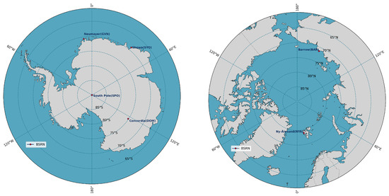
Figure 1.
BSRN polar station locations: (a) Antarctica and (b) Arctic. The acronyms in parentheses indicate the official BSRN station labels.
As shown in Table 1, only the decade between 2010 and 2020 is analyzed, as 2010 was the start of measurements of the upwelling components at DOM, the last Antarctic station to join the BSRN network. It is important to note that BSRN applies rigorous quality control procedures before data are published on platforms such as PANGAEA. These procedures follow a standardized station-to-archive format to ensure that only high-quality, validated measurements are included in the final dataset. Quality checks are performed using the official BSRN Toolbox [42], which combines automated and manual methods to identify and flag suspect or erroneous data.
Thanks to the direct measurement of all components of SW and LW broadband radiation, it is possible to use the RADFLUX package to obtain CF estimates. Although upwelling components are not needed by RADFLUX, the upwelling thermal component (LWU) can be useful to evaluate cloud conditions, especially to identify overcast situations because ground and cloud bottom temperature are similar, and therefore, the difference between LWD and LWU is close to 0.
2.2. RADFLUX
The RADFLUX [28] algorithm relies on both SW and LW broadband radiation measurements. In particular, it needs SWD, DIF, and LWD components, along with and relative humidity (RH) observations in order to yield estimates for clear sky (CS) SWD, LWD, and cloud fraction.
The RADFLUX procedure is divided into four parts: the first quality checks the measurements according to [43], the second performs a cloud screening of measurements and evaluates SWDCS [44], the third computes CF according to [27], and the fourth processes the LWD measurements to estimate LWDCS and CF according to [26,45]. Cloud screening and cloud fraction computation are based on a series of threshold values for the observations and derived variables; a complete description of the algorithms can be found in the respective papers mentioned above. A brief summary of the algorithm behind the shortwave and longwave code sections to obtain CF will be given.The algorithm uses four different tests to flag measurements as clear-sky or cloudy. Then, day by day, the identified clear sky measurements are used to obtain the A and b coefficients to parameterize both the clear sky global and diffuse components of SW according to [44]. Coefficients for cloudy days (i.e., those with an insufficient number of clear sky measurements) are then interpolated. Cloud fraction is obtained using an equation () derived through the comparison, with retrievals from a hemispherical sky imager [27]. The equation is based on the normalized downward diffuse cloud effect , defined as , and takes into account the sensibility of the diffuse component to the presence of clouds. CF is computed after screening first for overcast cases. Similar to the shortwave part of the code, for evaluating CF from LWD observations, first, one needs to estimate the clear sky component, and second, this is used in combination with observations to compute the cloud fraction. LWDCS is obtained using a modified version [45] of the parametrization by [46], which exploits surface temperature and relative humidity to derive the clear sky thermal component. In particular, Brutsaert’s parametrization correlates the clear sky emissivity to the ratio between water vapor pressure and air surface temperature . Cloud fraction is then obtained according to the scheme by the APCADA algorithm [26], which assigns a cloud amount based on the cloud-free index (ratio of actual emissivity to clear sky emissivity) and the variability of LWD. The actual emissivity is computed as , where is the Stefan–Boltzmann constant. The authors of [47] pointed out the good climatological correlation between total water vapor and surface temperature, as was also subsequently noted in [48]. Moreover, because of Brutsaert’s parametrization, the ratio of water vapor pressure to is considered one of the features in the classification task for ML algorithms.
As mentioned, CF is obtained from both SW and LW data; this means that the labels to classify the sky conditions can be either based on CF(SW) or CF(LW). There is no clear agreement between authors on what would be the optimal thresholds for such indicators, nor on whether such universal optimal thresholds exist [49]. For the purpose of this work, the clear sky conditions label (CS) is used for all measurements that correspond to a CF smaller than 0.1, as values of 0 denote cloud-free sky conditions; the cloudy (CL) conditions label is given to measurements that correspond to a CF in between 0.1 and 0.9, and the overcast (OC) label is used to denote measurements whose CF is larger than 0.9, as 1 is the value for overcast sky conditions. The labels based on SW measurements are considered more reliable, although they are limited only to the periods of sunlight and with a solar zenith angle (SZA) smaller than 80°, as it is possible to infer from the variation of the observations in time whether clouds were present; moreover, components of SW radiation are sensitive to even small variations in cloud cover and type [50]. Labels based on LW measurements have the known limitation of not including cirrus clouds (if present), as this type of cloud has little effect on LWD and, therefore, is typically not detected by methods based on LW radiation. Moreover, in the high Antarctic plateau region, the strong temperature inversion phenomena usually mask the LW fluxes at the surface, leading to strong uncertainties in cloud retrieval [51].
2.3. Classification Task
This work leverages the physical information contained in both SW and LW radiation measurements to enable established machine learning models to accurately classify sky conditions computed with RADFLUX. The feature set used for training includes LWD, , RH, the ratio of water vapor pressure with respect to , and SZA. Additionally, to supervise the training of the machine learning algorithms, a labeling strategy was adopted that prioritizes the more reliable SW radiation data. As discussed in the previous section, labels derived from SW measurements are considered more trustworthy. Therefore, the cloud fraction used for labeling is computed using SW data when available, defaulting to LW measurements only when SW data is missing. However, during inference, the label is derived exclusively from SW-based measurements to ensure consistency and reliability.
The analysis follows a two-step approach. First, classification performance is evaluated at each station using a leave-one-year-out strategy that is derived from the conventional leave-one-out cross-validation approach [52]. In this case, the model is trained on data from all years except one and tested on the excluded year. This process is repeated for each year in the dataset, enabling a robust assessment of the model’s ability to generalize across different temporal conditions at individual stations. In this setup, the model is trained and tested on data from the same station, using a training set of 100,000 samples. For each available year, the test is conducted by excluding all data from that specific year during training, using it exclusively for testing. Second, the generalization capability of the machine learning algorithms is assessed. Each station contributes a training set of 100,000 samples, and the resulting models are evaluated on the full dataset from the remaining stations, testing their ability to generalize across different locations.
The algorithms employed in this study are K-Nearest Neighbors (KNN) [53], Random Forest [54], and XGBoost [55]. KNN is a simple, instance-based learning method that classifies samples based on the majority label among their nearest neighbors in the feature space. Random Forest is an ensemble method that builds multiple decision trees and aggregates their predictions to improve accuracy and reduce overfitting. XGBoost is a gradient boosting framework that builds additive models in a forward stage-wise procedure, optimizing for both performance and computational efficiency. The KNN and Random Forest models are implemented using the Scikit-learn library [56], while the XGBoost model is implemented using the XGBoost Python package (2.1 release) [57].
Each of these algorithms requires careful tuning of its hyperparameters to achieve optimal performance. The best hyperparameters for each algorithm are selected using an internal 5-fold cross-validation with the GridSearchCV [58] function from the Scikit-learn Python library. Specifically, each training set is divided into 5 uniform subsets, with 4 subsets used for training and the remaining one for validation. This process is repeated 5 times, ensuring that each subset is used as the validation set exactly once. For each combination of hyperparameters in the specified search space, the model is trained and validated 5 times. The parameter set that achieves the best results is then selected for the final training, which is performed once more using the entire available training data. Balanced accuracy [59] is used as the evaluation metric throughout this process. It is defined as the average of the recall obtained on each class, making it particularly suitable for imbalanced classification problems, as it accounts for performance across all classes equally. For the K-Nearest Neighbors algorithm, the number of neighbors and the weighting strategy were considered. The number of neighbors was tested with values of 3, 5, and 10, reflecting different levels of locality in the decision boundary. The weighting strategy was varied between uniform, where each neighbor contributes equally to the classification, and distance, where closer neighbors have a stronger influence. For Random Forest and XGBoost, the hyperparameters included the number of estimators and the maximum tree depth. The number of estimators, which controls the number of decision trees in the ensemble, was set to 5, 10, 50, and 100. The maximum tree depth, which limits the growth of each tree, was tested with values of 3, 5, and None (unlimited depth).
To visually assess the distribution of key input features across different BSRN stations, in Figure 2, histograms are reported for five selected variables: longwave downward radiation (LWD), solar zenith angle (SZA), surface temperature (Ts), relative humidity (RH), and ratio. For each feature, data from the six BSRN polar stations were plotted on the same axis to facilitate direct comparison. Prior to plotting, basic filtering was applied to remove extreme or non-physical values. This visualization highlights station-specific shifts and variations in feature distributions, which are critical for interpreting model behavior and for guiding the application of normalization strategies.
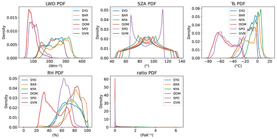
Figure 2.
Kernel Density Estimate (KDE) plots illustrate the distributions of five input features—longwave downwelling radiation (LWD), solar zenith angle (SZA), surface temperature (Ts), relative humidity (RH), and the vapor pressure-to-temperature ratio—across all six BSRN stations. Each subplot presents the KDEs for a specific feature, highlighting variations in local climate conditions and the range of observed data at each station.
Because the scales of the input variables differ significantly, it is often beneficial to normalize them. Without normalization, features with larger numerical ranges can dominate the learning process, particularly for algorithms that rely on gradient descent or distance-based methods like KNN, potentially leading to skewed or suboptimal outcomes.
A common normalization technique rescales each feature f to the range using its minimum and maximum values, and , respectively, as follows:
Typically, and are computed from the training set and then used to normalize both training and test data. This approach assumes that the training and test sets follow the same distribution, which is a reasonable assumption when both sets are drawn from the same station.
However, in cross-station scenarios, this assumption no longer holds. As shown in Figure 2, environmental conditions vary significantly between stations, resulting in markedly different distributions for the same variable. In such cases, using a single normalization scale derived from the training data can distort the feature space of the test set, leading to poor generalization.
To address this, features that exhibit substantial cross-station variability should be normalized independently within each domain. That is, and should be calculated separately for the training and test sets, and each set should be normalized using its own values. This relative normalization approach maps the values within each station to the same range, preserving their local structure and allowing models to focus on intra-domain patterns rather than being misled by inter-domain shifts.
In this study, relative normalization was applied to surface temperature (Ts), longwave downward radiation (LWD), and the ratio variable, all of which demonstrated consistent but shifted distributions across stations.
3. Results
3.1. RADFLUX Cloud Fraction Distribution
The CF used for labeling is computed from shortwave (SW) data when available, with longwave (LW) measurements used as a fallback when SW data are unavailable. The percentage of valid data resulting from this selection is reported in Table 2.
Table 2.
Summary of the dataset composition, including the total number of data points, the percentage of non-missing and non-outlier values in the combined label column, and the proportion of labels derived from SWlabel and LWlabel based on RADFLUX calculations.
The distribution of CF for the decade 2010–2020, gathered in 0.1 bins, is shown in Figure 3 for both the Arctic and Antarctica. In Figure 3, CF (LW) (yellow) represents the annual sky conditions, whereas CF(SW) (purple) and CF(LW) SZA < 80° (red) represent daylight results.
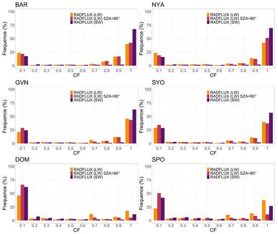
Figure 3.
Annual distribution of estimated CF by RADFLUX in 0.1 bins based on 10 years of SW and LW observations for Arctic and Antarctic stations. The LW classification with SZA < 80° refers to both polar night and low solar elevation.
Furthermore, as mentioned in Section 2.2, the sky condition labels are determined based on cloud fraction (CF) values. Specifically, clear sky (CS) conditions are assigned to all measurements with a CF of less than 0.1, as a value of 0 indicates a completely cloud-free sky. Cloudy (CL) conditions correspond to CF values between 0.1 and 0.9, and the overcast label (OC) is applied when CF exceeds 0.9, as a CF of 1 denotes fully overcast conditions. The resulting label distributions, separated by CF values derived from SW and LW data, are shown for each station in Figure 4.
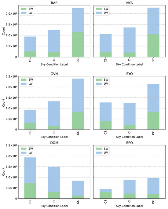
Figure 4.
Distribution of sky condition labels in the dataset, computed from RADFLUX, depicting the frequency of each category: clear sky (CS), cloudy (Cl), and overcast (OC). The counts reflect the total occurrences of each label across all data samples. The stacked bars distinguish between labels derived from SW and LW cloud fraction values, with SW used when available and LW as a fallback.
3.2. Features Importance
For the tree-based models, a feature importance analysis was performed to evaluate the contribution of each feature and to identify potential station-specific patterns. Figure 5 displays the feature importance values for the Random Forest algorithm trained with data from each station.
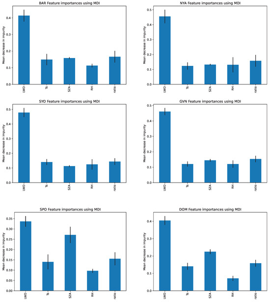
Figure 5.
Feature importance scores from the Random Forest classifier training data for each BSRN station. The results refer to the best-performing configuration, which uses selective relative normalization. The plots highlight the most influential features contributing to model predictions at each station.
3.3. Leave-One-Year-Out Analysis
The leave-one-year-out analysis was employed to evaluate the temporal generalization capability of the machine learning models. In this approach, data from one specific year is withheld as the test set, while the models are trained on the remaining years. In Figure 6, the performance of each station over different test years is presented.
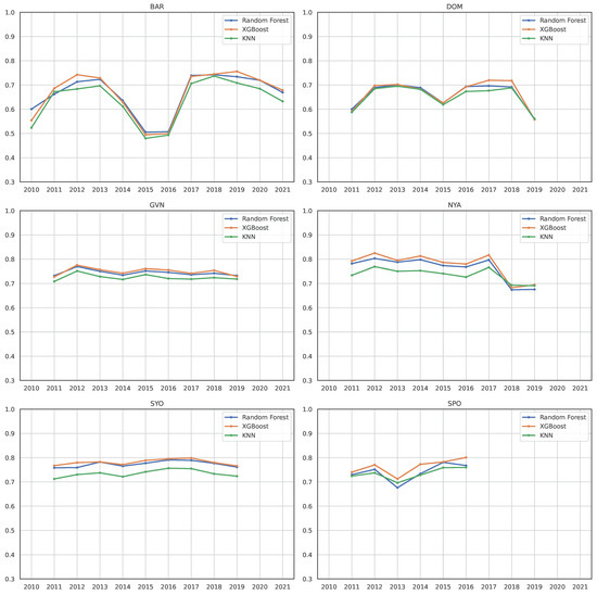
Figure 6.
Leave-one-year-out temporal analysis for BSRN stations, used to evaluate model generalization over time by training on all years except one and testing on the excluded year. The results are reported in terms of balanced accuracy.
In Table 3, the overall performance of each model across different stations in terms of balanced accuracy, weighted precision, recall, and F1 score is presented. While balanced accuracy gives an overall measure of classification effectiveness, weighted precision and recall emphasize the model’s ability to correctly identify each class, accounting for their prevalence. The weighted F1 score further balances these aspects, combining both precision and recall into a single metric.
Table 3.
Leave-one-year-out analysis on models and stations: balanced accuracy, weighted precision, recall, and F1 scores are reported to assess the temporal generalization of each model across different BSRN stations.
3.4. Cross-Station Analysis
Figure 7 presents the balanced accuracy of each model across all stations. For each model, a heatmap compares absolute normalization (left) with selective relative normalization (right). The features selected for relative normalization—surface temperature (Ts), ratio, and longwave downward radiation (LWD)—were chosen based on their similar overall distributions across stations, despite exhibiting location-specific shifts, as shown in Figure 2.
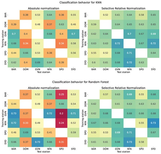
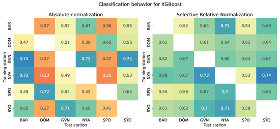
Figure 7.
Balanced accuracy across all stations for the three classification models: KNN, Random Forest, and XGBoost. Each panel compares absolute normalization (left) with selective relative normalization (right), where relative normalization is applied to surface temperature (Ts), longwave downward radiation (LWD), and the ratio.
4. Discussion
4.1. Sky Condition in Arctic and Antarctic BSRN Stations
The results from the Arctic sites BAR and NYA are very similar, with a prevalence of OC cases (overall, more than 40% and up to 70% when considering SW only) over CS conditions (between 20 and 25%). Another 20–25% accounts for a CF of between 0.8 and 0.9. For the Antarctic sites, the results for the coastal stations GVN and SYO are similar to those from the Arctic (and between them), while the Eastern Antarctic Plateau stations DOM and SPO show much more CS cases—between 50 and 70% for the first and up to 50% for the latter, and much less OC cases, with 20–25% maximum for SPO and fewer for DOM. This reflects the peculiar sky condition over the Antarctic Plateau (SPO is slightly cloudier than DOM).
Except for the stations on the plateau, where sky conditions are cloudier when also considering polar night measurements, there seems to be no strong seasonal dependence of CF distribution over the whole decade. The differences between the CF obtained using SW and LW observations can be attributed to both the different sensibilities of the methods to cloud type and cover, as well as the different cloud screening methods of the algorithms for the different components.
4.2. Feature Importance
Feature importance scores from the Random Forest classifier training data are presented for each BSRN station, based on the best-performing configuration that employs selective relative normalization. As shown in Figure 5, the most influential features are highlighted across the three models, illustrating their respective contributions to predictions at each site. It can be observed that the main contribution to the classification task is provided by LWD across all stations. Notably, SZA also plays a more significant role at the SPO and DOM stations. In Antarctica, the solar zenith angle (SZA) is a critical factor due to its pronounced annual variability [60]. SZA increases with latitude, meaning stations closer to the geographic South Pole experience higher values and are characterized by relatively small fluctuations in SZA (at SPO, there is almost no appreciable daily variation throughout the polar day), which may impact the accuracy of RADFLUX calculations. In contrast to coastal regions, where albedo varies significantly due to changing surface types, DOM displays minimal surface variability [61]. This makes it a particularly unique case, as both the stability in albedo and limited SZA variation reduce the dynamic range of radiative inputs, potentially influencing model sensitivity and performance.
4.3. Leave-One-Year-Out Analysis
The results shown in Table 3 highlight several key patterns in model performance across different BSRN stations under a leave-one-year-out temporal validation framework. Overall, XGBoost consistently ranks as the best-performing model across all evaluated metrics and stations. Random Forest also demonstrates strong performance, closely trailing behind XGBoost, while KNN consistently records the lowest scores, particularly at stations such as DOM and BAR. Stations like GVN, NYA, and SYO exhibit the highest overall performance, suggesting more stable and predictable temporal patterns. In contrast, the DOM and SPO stations pose greater challenges for modeling, as reflected in their lower precision, recall, and F1 scores. Balanced accuracy follows a similar trend, with XGBoost achieving the highest values, especially at NYA and SYO, where scores reach 0.74 and 0.73, respectively. All models maintained balanced accuracies above 0.70 for four out of the six stations. However, balanced accuracy slightly declined to a minimum of 0.65 with KNN at the DOM station and reached a maximum of 0.69 for the tree-based models at BAR.
Finally, in Figure 6, the performances of each station over different test years are presented. Most stations exhibit a relatively stable, balanced accuracy, with only minor variations from year to year. Specifically, for the Arctic, station NYA reports balanced accuracies below 0.7 only for 2018 and 2019. For BAR, we observe a sharp drop in performance in 2015 and 2016. As shown in Figure 8, this drop coincides with a lack of radiation measurements during those years, which is unlike other years where radiation data is uniformly available throughout the observation period.
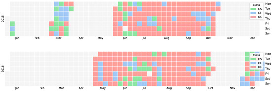
Figure 8.
Sky condition labels based on daily mean computed using RADFLUX for BAR. Legend indicates the following classes: clear sky, cloudy, and overcast.
Furthermore, as shown in Figure 9, LW radiation measurements for the years 2015 and 2016 deviate significantly from the average, suggesting increased cloud cover compared to other periods. On the other hand, Antarctic stations exhibit a relatively stable, balanced accuracy. The only notable exception is DOM, which shows a slight decline in 2011 and 2015 and a more pronounced drop in 2019. However, in this case, data availability remains consistent throughout the period (as shown in Figure 10). Although LW radiation measurements are slightly below the mean, the deviation is not as pronounced (Figure 11), and the corresponding drop in classification accuracy is less severe compared to BAR.
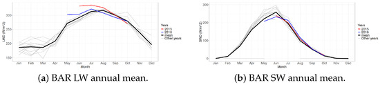
Figure 9.
Annual mean radiation measurements at the BAR station: (a) LW and (b) SW components.
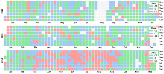
Figure 10.
Sky condition labels based on daily mean computed using RADFLUX for DOM. Legend indicates the following classes: clear sky, cloudy, and overcast.
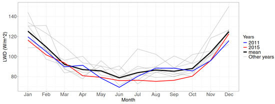
Figure 11.
Longwave annual mean at the DOM station, used for the computation of cloud fraction.
Lastly, as already noted in Table 3, the tested models yield similar values for balanced accuracy. KNN consistently ranks as the lowest-performing model, with only minor variations—except at the NYA and SYO stations, where the performance gap becomes more noticeable.
4.4. Cross-Station Analysis
As shown in Figure 7, the cross-station classification results are presented under the two normalization strategies described in Section 2.3: (i) absolute normalization, applied uniformly across all features, and (ii) selective relative normalization, applied only to a subset of features.
For each of the three models, each of the left heatmaps in Figure 7 reveals several notable patterns in cross-station classification performance under absolute normalization. In particular, models trained on stations such as GVN and SYO exhibit good generalization, achieving (using KNN) high balanced accuracy when tested on other stations; for example, GVN → SYO reaches 0.70, while SYO → GVN scores 0.69. This behavior is likely influenced by the fact that both stations are located along the Antarctic coast, as shown in Figure 4, confirming that they experience similar environmental conditions. These geographic and climatic similarities likely enhance the model’s ability to transfer learned patterns effectively, even in the absence of parameter-specific normalization. Similarly, in the Arctic region, a strong correspondence is observed between NYA and BAR, with BAR → NYA achieving 0.73 and NYA → BAR scoring 0.67 with XGBoost. These findings further support the idea that shared environmental characteristics among stations can enhance cross-station model transferability. Moreover, they underscore that the relatively good performance under absolute normalization is largely dependent on geographic similarity since absolute normalization alone fails to consistently harmonize differences across stations when environmental conditions diverge. DOM, in particular, appears to be a challenging target station, receiving consistently low scores regardless of the training source. Situated on the Antarctic Plateau, this station is subject to extremely low temperatures and demonstrates significant alignment only with SPO, which experiences similarly harsh conditions. This is evident in their cross-station performance, with 0.66 when using KNN, 0.69 when using Random Forest, and 0.72 when using XGBoost. These results suggest that, under this strategy, the success of cross-station classification heavily depends on the similarity between the training and test stations. This similarity is crucial for the assumptions underlying absolute normalization to hold. In cross-station settings, however, feature values can vary significantly in scale due to differing environmental conditions. When such variations are not accounted for, machine learning models may struggle to generalize, leading to degraded performance.
To account for this, a relative normalization approach is also adopted, allowing models to better adapt to local variations within each dataset, targeting only features that require adjustment to ensure consistent representation during training: surface temperature (Ts), ratio, and longwave downward radiation (LWD). The most notable difference in the right panel of Figure 7, focused on selective relative normalization, is the overall improvement in classification accuracy compared to absolute normalization. For each model in the right heatmap, nearly all cells exhibit higher values than their counterparts on the left, indicating that selective relative normalization enhances the model’s ability to generalize across stations. Indeed, the heatmaps for selective relative normalization highlight how the models generally have a lower variance in the obtained accuracies, maintaining reliable performance regardless of which stations are being compared. In contrast, the absolute normalization heatmap displays greater variability, with classification performance fluctuating significantly across different station combinations. Notably, station pairs that performed poorly under absolute normalization, such as GVN → DOM (0.40) and SPO → BAR (0.44), show marked improvement with selective relative normalization, rising to 0.64 and 0.55, respectively, with KNN. Even the relatively strong performances under absolute normalization are largely preserved; although a few peak values may be slightly reduced, the overall performance baseline is substantially elevated.
5. Conclusions
The polar regions exhibit a high degree of climate sensitivity and are subject to considerable natural variability. In recent decades, the Arctic has experienced warming at more than twice the global average rate, accompanied by a consistent decline in sea ice across all months, with the most pronounced losses occurring in late summer. Conversely, the Antarctic shows a more complex pattern, with some areas warming and losing sea ice, while others have seen cooling and even increases in sea ice extent. The observed changes in polar climates result from complex interactions among atmospheric conditions, ocean dynamics, sea ice, and terrestrial surfaces. However, our understanding of these processes remains limited due to their inherent complexity and the scarcity of available observational datasets [62].
Monitoring cloud fraction (CF) trends is especially important for detecting early indicators of climate change in these sensitive regions, where clouds can either amplify or moderate warming depending on the season and prevailing atmospheric conditions. Direct observation of clouds is particularly challenging, and this makes the development of reliable methods to estimate cloud cover and its impact on radiative fluxes using simple broadband radiation instruments both valuable and practical. Satellite observations, although widely used, face limitations in polar regions, where distinguishing clouds from snow and ice is difficult due to their similar optical and thermal properties. All-sky cameras are a promising option, but they are still under development. Human observations—known as synoptic reports—are infrequent and subjective, and instrument-based measurements are often difficult to perform and maintain in the harsh polar environment. At BSRN stations, instruments are routinely inspected and cleaned. When ice formation is known, the affected data are removed. In some cases, ice can be identified through redundancy protocols, which check for internal consistency among multiple measurements. However, not all instances can be detected. At unattended stations, this becomes a significant issue. To address this, a solution under discussion within the BSRN community is the use of webcams to monitor instrument conditions in real time.
This complexity characterizes both the Arctic and Antarctic environments, and this work aims to address the problem through a bipolar approach by considering BSRN stations from both poles. Emphasizing the unique advantages of machine learning (ML) in polar cloud analysis could significantly influence future research directions, as supported by recent studies [13,63]. From this perspective, incorporating data from both polar regions is essential for developing a generalizable model that captures a broader range of atmospheric scenarios, thereby enhancing its robustness and applicability to stations beyond the BSRN network across diverse polar environments. In fact, adopting a bipolar approach requires careful consideration of several key factors. Nevertheless, caution needs to be taken when directly comparing stations in the Arctic and Antarctic, as it can lack meaningful interpretation due to the fundamentally different climatic, geographic, and environmental conditions that characterize these two polar regions [64]. Notably, the primary differences between BSRN stations in the Arctic and Antarctic stem from variations in snow characteristics, seasonal cycles, and the distinct processes influencing surface radiation and albedo [65]. These differences are crucial not only for interpreting BSRN radiation data but also for understanding the surface energy budget in polar climates. Incorporating ancillary variables such as temperature, humidity, solar zenith angle (SZA), and vapor pressure-to-temperature ratio further helps to characterize and differentiate each pole’s environmental scenarios more accurately.
The machine learning methods employed in this study demonstrate solid overall accuracy and show promise for developing station-specific models, which are particularly valuable for predicting sky conditions in the absence of ancillary variables. While tailoring models to individual stations can produce strong results, building more generalizable models is especially meaningful when applied to clusters of stations that share similar environmental and climatic characteristics. To further enhance model robustness and generalization, future work should incorporate additional non-BSRN stations from both the Arctic and Antarctic regions. In this context, incorporating additional non-BSRN stations such as Marambio (Antarctic Peninsula) and Jang Bogo (Terranova Bay) in future work could further enhance the robustness and generalizability of the analysis. A similar consideration applies when selecting ground-based meteorological stations across the continental Arctic, such as Narsaq (Greenland) and Gruvebadet (Svalbard Islands), which offer valuable observational data within comparable regional contexts.
Although a comprehensive comparison of cloud fraction retrieval methods falls outside the scope of this study, alternative approaches such as the Long and Ackerman method (LC) [44], APCADA [26], and the method proposed by Van Den Broeke [25,66] should also be considered. These methods detect clear-sky conditions using either longwave or shortwave radiation measurements. In this study, RADFLUX was selected due to its ability to assess sky conditions using both shortwave and longwave data. Future research could benefit from comparing the label sets generated by these different methods with those derived from RADFLUX and incorporating them into machine learning models to improve cloud detection and classification accuracy. Given that method selection is often limited by data availability, it is also important to include observations from non-BSRN stations, potentially sourced from other observational networks.
Author Contributions
Conceptualization, C.F., A.L., V.V. and A.C.; methodology, C.F., A.C., D.B. and D.S.; software, D.B., D.S. and C.F.; formal analysis, C.F., A.L., A.C., D.B. and D.S.; investigation, C.F., A.C., D.B., D.S. and A.L.; resources, C.F., A.L., D.B. and D.S.; data curation, C.F., A.L., A.C., D.B. and D.S.; writing—original draft preparation, C.F., A.C., D.B., D.S. and A.L.; writing—review and editing, C.F., A.L., A.C., D.S., M.B., M.M. and S.P.; visualization, M.B., M.M. and S.P. All authors have read and agreed to the published version of the manuscript.
Funding
This research received no external funding.
Institutional Review Board Statement
Not applicable.
Informed Consent Statement
Not applicable.
Data Availability Statement
All station datasets are available on PANGAEA [32].
Acknowledgments
The authors wish to thank Laura D. Riihimaki and Christopher Cox for the insight provided on how to use RADFLUX, and they acknowledge Charles N. Long for his RADFLUX code and work. Part of this work is supported by IR0000032 ITINERIS, Italian Integrated Environmental Research Infrastructures System (D.D. 130/2022—CUP B53C22002150006), funded by EU—Next Generation.
Conflicts of Interest
The authors declare no conflicts of interest.
Abbreviations
The following abbreviations are used in this manuscript:
| SW | shortwave |
| LW | longwave |
| Rnet | net broadband radiation/surface radiation budget |
| SWD | downwelling shortwave broadband radiation |
| SWU | upwelling shortwave broadband radiation |
| DIF | diffuse shortwave broadband radiation |
| LWD | downwelling longwave broadband radiation |
| LWU | upwelling longwave broadband radiation |
| SWDcs | estimated clear sky downwelling shortwave broadband radiation |
| LWDcs | estimated clear sky downwelling longwave broadband radiation |
| CF | cloud fraction |
| CF (SW) | cloud fraction as estimated with SW measurements |
| CF (LW) | cloud fraction as estimated with LW measurements |
| CS | clear sky conditions (label) |
| CL | cloudy sky conditions (label) |
| OC | overcast sky conditions (label) |
| BSRN | Baseline Surface Radiation Network |
| DOM | DomeC station |
| SPO | Amundsen-Scott South Pole station |
| GVN | Neumayer III station |
| SYO | Syowa station |
| NYA | Ny Ålesund station |
| BAR | Utqiaġvik (formerly Barrow) station |
References
- Ohmura, A. Observed decadal variations in surface solar radiation and their causes. J. Geophys. Res. Atmos. 2009, 114. [Google Scholar] [CrossRef]
- Lubin, D.; Ghiz, M.L.; Castillo, S.; Scott, R.C.; LeBlanc, S.E.; Silber, I. A Surface Radiation Balance Dataset from Siple Dome in West Antarctica for Atmospheric and Climate Model Evaluation. J. Clim. 2023, 36, 6729–6748. [Google Scholar] [CrossRef]
- Kasten, F.; Czeplak, G. Solar and terrestrial radiation dependent on the amount and type of cloud. Sol. Energy 1980, 24, 177–189. [Google Scholar] [CrossRef]
- Wang, G.; Wang, T.; Xue, H. Validation and comparison of surface shortwave and longwave radiation products over the three poles. Int. J. Appl. Earth Obs. Geoinf. 2021, 104, 102538. [Google Scholar] [CrossRef]
- Schäfer, B.; Carlsen, T.; Hanssen, I.; Gausa, M.; Storelvmo, T. Observations of cold-cloud properties in the Norwegian Arctic using ground-based and spaceborne lidar. Atmos. Chem. Phys. 2022, 22, 9537–9551. [Google Scholar] [CrossRef]
- Tom, L.C. Antarctic clouds. Polar Res. 2010, 29, 150–158. [Google Scholar] [CrossRef]
- Yabuki, M.; Shiobara, M.; Nishinaka, K.; Kuji, M. Development of a cloud detection method from whole-sky color images. Polar Sci. 2014, 8, 315–326. [Google Scholar] [CrossRef]
- Chen, Y.; Sun-Mack, S.; Arduini, R.F.; Hong, G.; Minnis, P. Predicting Clear-Sky Reflectance Over Snow/Ice in Polar Regions. In Proceedings of the International Symposium on Atmospheric Light Scattering and Remote Sensing, Wuhan, China, 1–4 June 2015. Number NF1676L-21013. [Google Scholar]
- Ganeshan, M.; Yang, Y.; Palm, S.P. Impact of clouds and blowing snow on surface and atmospheric boundary layer properties over Dome C, Antarctica. J. Geophys. Res. Atmos. 2022, 127, e2022JD036801. [Google Scholar] [CrossRef]
- Shi, T.; Clothiaux, E.E.; Yu, B.; Braverman, A.J.; Groff, D.N. Detection of daytime arctic clouds using MISR and MODIS data. Remote Sens. Environ. 2007, 107, 172–184. [Google Scholar] [CrossRef]
- Trepte, Q.; Minnis, P.; Arduini, R.F. Daytime and nighttime polar cloud and snow identification using MODIS data. In Proceedings of the Optical Remote Sensing of the Atmosphere and Clouds III; SPIE: Hangzhou, China, 2003; Volume 4891, pp. 449–459. [Google Scholar] [CrossRef]
- Wu, T.; Liu, Q.; Jing, Y. Cloud Screening Method in Complex Background Areas Containing Snow and Ice Based on Landsat 9 Images. Int. J. Environ. Res. Public Health 2022, 19, 13267. [Google Scholar] [CrossRef]
- Kumar, Y.; Kaul, S.; Sood, K. Effective use of the machine learning approaches on different clouds. In Proceedings of the International Conference on Sustainable Computing in Science, Technology and Management (SUSCOM), Amity University Rajasthan, Jaipur, India, 26–28 February 2019. [Google Scholar]
- Sedlar, J.; Riihimaki, L.D.; Lantz, K.; Turner, D.D. Development of a random-forest cloud-regime classification model based on surface radiation and cloud products. J. Appl. Meteorol. Climatol. 2021, 60, 477–491. [Google Scholar] [CrossRef]
- Kazantzidis, A.; Tzoumanikas, P.; Bais, A.; Fotopoulos, S.; Economou, G. Cloud detection and classification with the use of whole-sky ground-based images. Atmos. Res. 2012, 113, 80–88. [Google Scholar] [CrossRef]
- Poulsen, C.; Egede, U.; Robbins, D.; Sandeford, B.; Tazi, K.; Zhu, T. Evaluation and comparison of a machine learning cloud identification algorithm for the SLSTR in polar regions. Remote Sens. Environ. 2020, 248, 111999. [Google Scholar] [CrossRef]
- Zeng, Z.; Wang, Z.; Ding, M.; Zheng, X.; Sun, X.; Zhu, W.; Zhu, K.; An, J.; Zang, L.; Guo, J.; et al. Estimation and long-term trend analysis of surface solar radiation in Antarctica: A case study of zhongshan station. Adv. Atmos. Sci. 2021, 38, 1497–1509. [Google Scholar] [CrossRef]
- Anzalone, A.; Pagliaro, A.; Tutone, A. An Introduction to Machine and Deep Learning Methods for Cloud Masking Applications. Appl. Sci. 2024, 14, 2887. [Google Scholar] [CrossRef]
- Fu, Y.; Mi, X.; Han, Z.; Zhang, W.; Liu, Q.; Gu, X.; Yu, T. A Machine-Learning-Based Study on All-Day Cloud Classification Using Himawari-8 Infrared Data. Remote Sens. 2023, 15, 5630. [Google Scholar] [CrossRef]
- Yang, Y.; Sun, W.; Chi, Y.; Yan, X.; Fan, H.; Yang, X.; Ma, Z.; Wang, Q.; Zhao, C. Machine learning-based retrieval of day and night cloud macrophysical parameters over East Asia using Himawari-8 data. Remote Sens. Environ. 2022, 273, 112971. [Google Scholar] [CrossRef]
- Paul, S.; Huntemann, M. Improved machine-learning-based open-water–sea-ice–cloud discrimination over wintertime Antarctic sea ice using MODIS thermal-infrared imagery. Cryosphere 2021, 15, 1551–1565. [Google Scholar] [CrossRef]
- Sedona, R.; Hoffmann, L.; Spang, R.; Cavallaro, G.; Griessbach, S.; Höpfner, M.; Book, M.; Riedel, M. Exploration of machine learning methods for the classification of infrared limb spectra of polar stratospheric clouds. Atmos. Meas. Tech. 2020, 13, 3661–3682. [Google Scholar] [CrossRef]
- Fiddes, S.L.; Mallet, M.D.; Protat, A.; Woodhouse, M.T.; Alexander, S.P.; Furtado, K. A machine learning approach for evaluating Southern Ocean cloud radiative biases in a global atmosphere model. Geosci. Model Dev. 2024, 17, 2641–2662. [Google Scholar] [CrossRef]
- Kuma, P.; Bender, F.A.M.; Schuddeboom, A.; McDonald, A.J.; Seland, Ø. Machine learning of cloud types in satellite observations and climate models. Atmos. Chem. Phys. 2023, 23, 523–549. [Google Scholar] [CrossRef]
- Van Den Broeke, M.; Reijmer, C.; Van De Wal, R. Surface radiation balance in Antarctica as measured with automatic weather stations. J. Geophys. Res. Atmos. 2004, 109, 2003JD004394. [Google Scholar] [CrossRef]
- Dürr, B.; Philipona, R. Automatic cloud amount detection by surface longwave downward radiation measurements. J. Geophys. Res. Atmos. 2004, 109, 2003JD004182. [Google Scholar] [CrossRef]
- Long, C.N.; Ackerman, T.P.; Gaustad, K.L.; Cole, J.N.S. Estimation of fractional sky cover from broadband shortwave radiometer measurements. J. Geophys. Res. Atmos. 2006, 111, 2005JD006475. [Google Scholar] [CrossRef]
- Riihimaki, L.D.; Gaustad, K.L.; Long, C.N.; PNNL; BNL; ANL; ORNL. Radiative Flux Analysis (RADFLUXANAL) Value-Added Product: Retrieval of Clear-Sky Broadband Radiative Fluxes and Other Derived Values 2019. DOE/SC–ARM–TR–228, p. 1569477. Available online: https://www.arm.gov/publications/tech_reports/doe-sc-arm-tr-228.pdf (accessed on 1 May 2025). [CrossRef]
- Driemel, A.; Augustine, J.; Behrens, K.; Colle, S.; Cox, C.; Cuevas-Agulló, E.; Denn, F.M.; Duprat, T.; Fukuda, M.; Grobe, H.; et al. Baseline Surface Radiation Network (BSRN): Structure and data description (1992–2017). Earth Syst. Sci. Data 2018, 10, 1491–1501. [Google Scholar] [CrossRef]
- McArthur, L.J.B. Baseline Surface Radiation Network (BSRN) Operations Manual; Technical Report, WCRP-121, WMO/TD-No.1274; Baseline Surface Radiation Network: Geneva, Switzerland, 2005. [Google Scholar]
- Long, C.N.; Dutton, E.G. BSRN Global Network recommended QC Tests V 2.0. 2002. Available online: http://hdl.handle.net/10013/epic.38770.d001 (accessed on 1 May 2025).
- Baseline Surface Radiation Network (BSRN). BSRN Station Data Portal. 2024. Available online: https://dataportals.pangaea.de/bsrn/stations (accessed on 14 May 2025).
- Riihimaki, L. BSRN Station No. 22—Barrow, Alaska. Surface Type: Tundra; Topography: Flat, Rural; Station Scientist: Laura Riihimaki (laura.riihimaki@noaa.gov). Available online: http://www.esrl.noaa.gov/gmd/obop/brw/ (accessed on 4 May 2025).
- Maturilli, M. BSRN Station No. 11—Ny-Ålesund, Svalbard. Surface Type: Tundra; Topography: Mountain Valley, Rural; Horizon Data; Alfred Wegener Institute—Research Unit: Potsdam, Germany, 2007; Station Scientist: Marion Maturilli (marion.maturilli@awi.de). Available online: https://doi.pangaea.de/10.1594/PANGAEA.669522 (accessed on 8 January 2025).
- Lupi, A. BSRN Station No. 74—Dome C, Antarctica. Surface Type: Glacier, Accumulation Area; Topography: Flat, Rural; Horizon Data; Institute of Atmospheric Sciences and Climate of the Italian National Research Council: Bologna, Italy, 2022; Station Scientist: Angelo Lupi (a.lupi@isac.cnr.it). Available online: https://doi.pangaea.de/10.1594/PANGAEA.947046 (accessed on 8 January 2025).
- Schmithüsen, H. BSRN Station No. 13—Neumayer, Antarctica (1992–2009-01). Surface Type: Iceshelf; Topography: Flat, rural; Horizon Data; Alfred Wegener Institute, Helmholtz Centre for Polar and Marine Research: Bremerhaven, Germany, 2020; Station scientist: Holger Schmithüsen (Holger.Schmithuesen@awi.de). Available online: https://doi.pangaea.de/10.1594/PANGAEA.669516 (accessed on 8 January 2025).
- Schmithüsen, H. BSRN Station No. 13—Neumayer, Antarctica (after 2009-01). Surface Type: Iceshelf; Topography: Flat, rural; Horizon Data; Alfred Wegener Institute, Helmholtz Centre for Polar and Marine Research: Bremerhaven, Germany, 2020; Station Scientist: Holger Schmithüsen (Holger.Schmithuesen@awi.de). Available online: https://doi.pangaea.de/10.1594/PANGAEA.757811 (accessed on 8 January 2025).
- Tanaka, Y. BSRN Station No. 17—Syowa, Antarctica (Original). Surface Type: Sea Ice; Topography: Hilly, Rural; Horizon Data; National Institute of Polar Research, Tokyo: Tokyo, Japan, 2007; Station Scientist: Yoshinobu Tanaka (antarctic@met.kishou.go.jp). Available online: https://doi.pangaea.de/10.1594/PANGAEA.669525 (accessed on 8 January 2025).
- Tanaka, Y. BSRN Station No. 17—Syowa, Antarctica (update 2017-01). Surface Type: Sea Ice; Topography: Hilly, Rural; Horizon Data; National Institute of Polar Research, Tokyo: Tokyo, Japan, 2007; Station Scientist: Yoshinobu Tanaka (antarctic@met.kishou.go.jp). Available online: https://doi.pangaea.de/10.1594/PANGAEA.948519 (accessed on 8 January 2025).
- Tanaka, Y. BSRN Station No. 17—Syowa, Antarctica (update 2020-03). Surface Type: Sea Ice; Topography: Hilly, Rural; Horizon Data; National Institute of Polar Research, Tokyo: Tokyo, Japan, 2007; Station Scientist: Yoshinobu Tanaka (antarctic@met.kishou.go.jp). Available online: https://doi.pangaea.de/10.1594/PANGAEA.948521 (accessed on 8 January 2025).
- Riihimaki, L. BSRN Station No. 26—South Pole, Antarctica. Surface Type: Glacier, Accumulation Area; Topography: Flat, Rural; Station Scientist: Laura Riihimaki (laura.riihimaki@noaa.gov). Available online: https://gml.noaa.gov/obop/spo/ (accessed on 8 January 2025).
- Schmithüsen, H.; Koppe, R.; Sieger, R.; König-Langlo, G. BSRN Toolbox V2.5—A Tool to Create Quality Checked Output Files from BSRN Datasets and Station-to-Archive Files; Alfred Wegener Institute, Helmholtz Centre for Polar and Marine Research: Bremerhaven, Germany, 2019. [Google Scholar] [CrossRef]
- Long, C.N.; Shi, Y. An Automated Quality Assessment and Control Algorithm for Surface Radiation Measurements. Open Atmos. Sci. J. 2008, 2, 23–37. [Google Scholar] [CrossRef]
- Long, C.N.; Ackerman, T.P. Identification of clear skies from broadband pyranometer measurements and calculation of downwelling shortwave cloud effects. J. Geophys. Res. Atmos. 2000, 105, 15609–15626. [Google Scholar] [CrossRef]
- Long, C.N.; Turner, D.D. A method for continuous estimation of clear-sky downwelling longwave radiative flux developed using ARM surface measurements. J. Geophys. Res. Atmos. 2008, 113, 2008JD009936. [Google Scholar] [CrossRef]
- Brutsaert, W. On a derivable formula for long-wave radiation from clear skies. Water Resour. Res. 1975, 11, 742–744. [Google Scholar] [CrossRef]
- Deacon, E.L. The derivation of Swinbank’s long-wave radiation formula. Q. J. R. Meteorol. Soc. 1970, 96, 313–319. [Google Scholar] [CrossRef]
- King, J. Longwave atmospheric radiation over Antarctica. Antarct. Sci. 1996, 8, 105–109. [Google Scholar] [CrossRef]
- Correa, L.F.; Folini, D.; Chtirkova, B.; Wild, M. A Method for Clear-Sky Identification and Long-Term Trends Assessment Using Daily Surface Solar Radiation Records. Earth Space Sci. 2022, 9, e2021EA002197. [Google Scholar] [CrossRef]
- Duchon, C.E.; O’Malley, M.S. Estimating Cloud Type from Pyranometer Observations. J. Appl. Meteorol. 1999, 38, 132–141. [Google Scholar] [CrossRef]
- Frangipani, C. Analysis of the Radiation Budget and Cloud Conditions over the Antarctic Region Using Ground Observations. Ph.D. Thesis, University G. d’Annunzio, Chieti-Pescara, Italy, 2025. [Google Scholar]
- Witten, I.H.; Frank, E.; Hall, M.A.; Pal, C.J.; Data, M. Practical machine learning tools and techniques. In Data Mining; Elsevier: Amsterdam, The Netherlands, 2005; Volume 2, pp. 403–413. [Google Scholar]
- Roweis, S.; Hinton, G.; Salakhutdinov, R. Neighbourhood component analysis. Adv. Neural Inf. Process. Syst.(NIPS) 2004, 17, 4. [Google Scholar]
- Breiman, L. Random forests. Mach. Learn. 2001, 45, 5–32. [Google Scholar] [CrossRef]
- Chen, T.; Guestrin, C. XGBoost: A Scalable Tree Boosting System. In Proceedings of the 22nd ACM SIGKDD International Conference on Knowledge Discovery and Data Mining, KDD ’16, San Francisco, CA, USA, 13–17 August 2016; ACM: New York, NY, USA, 2016; pp. 785–794. [Google Scholar] [CrossRef]
- Pedregosa, F.; Varoquaux, G.; Gramfort, A.; Michel, V.; Thirion, B.; Grisel, O.; Blondel, M.; Prettenhofer, P.; Weiss, R.; Dubourg, V.; et al. Scikit-learn: Machine Learning in Python. J. Mach. Learn. Res. 2011, 12, 2825–2830. [Google Scholar]
- XGBoost Contributors. XGBoost Python Package. 2024. Available online: https://xgboost.readthedocs.io/en/latest/python/index.html (accessed on 15 April 2025).
- Bergstra, J.; Bengio, Y. Random search for hyper-parameter optimization. J. Mach. Learn. Res. 2012, 13, 281–305. [Google Scholar]
- Kelleher, J.D.; Mac Namee, B.; D’arcy, A. Fundamentals of Machine Learning for Predictive Data Analytics: Algorithms, Worked Examples, and Case Studies; MIT Press: Cambridge, MA, USA, 2020. [Google Scholar]
- Szymszová, S.; Láska, K.; Kim, S.J.; Park, S.J. Variability of solar radiation and cloud cover in the Antarctic Peninsula region. Atmos. Res. 2025, 316, 107940. [Google Scholar] [CrossRef]
- Carter, J.; Leeson, A.; Orr, A.; Kittel, C.; Van Wessem, J.M. Variability in Antarctic surface climatology across regional climate models and reanalysis datasets. Cryosphere 2022, 16, 3815–3841. [Google Scholar] [CrossRef]
- Goosse, H.; Kay, J.E.; Armour, K.C.; Bodas-Salcedo, A.; Chepfer, H.; Docquier, D.; Jonko, A.; Kushner, P.J.; Lecomte, O.; Massonnet, F.; et al. Quantifying climate feedbacks in polar regions. Nat. Commun. 2018, 9, 1919. [Google Scholar] [CrossRef] [PubMed]
- Bente, K. Probabilistic Machine Learning in Polar Earth and Climate Science: A Review of Applications and Opportunities. In AAAI 2022 Fall Symposium: The Role of AI in Responding to Climate Challenges; Westin Arlington Gateway: Arlington, VA, USA, 2022. [Google Scholar]
- Walsh, J.E. A comparison of Arctic and Antarctic climate change, present and future. Antarct. Sci. 2009, 21, 179–188. [Google Scholar] [CrossRef]
- Wang, X.; Zender, C.S. Arctic and Antarctic diurnal and seasonal variations of snow albedo from multiyear Baseline Surface Radiation Network measurements. J. Geophys. Res. Earth Surf. 2011, 116. [Google Scholar] [CrossRef]
- Van den Broeke, M.; Reijmer, C.; Van As, D.; Boot, W. Daily cycle of the surface energy balance in Antarctica and the influence of clouds. Int. J. Climatol. 2006, 26, 1587–1605. [Google Scholar] [CrossRef]
Disclaimer/Publisher’s Note: The statements, opinions and data contained in all publications are solely those of the individual author(s) and contributor(s) and not of MDPI and/or the editor(s). MDPI and/or the editor(s) disclaim responsibility for any injury to people or property resulting from any ideas, methods, instructions or products referred to in the content. |
© 2025 by the authors. Licensee MDPI, Basel, Switzerland. This article is an open access article distributed under the terms and conditions of the Creative Commons Attribution (CC BY) license (https://creativecommons.org/licenses/by/4.0/).