Regime Change in Top of the Atmosphere Radiation Fluxes: Implications for Understanding Earth’s Energy Imbalance

Abstract

Earth’s energy imbalance (EEI) is a major indicator of climate change. Its metrics are top of the atmosphere radiation imbalance (EEI TOA) and net internal heat uptake. Both EEI and temperature are expected to respond gradually to forcing on annual timescales. This expectation was tested by analyzing regime changes in the inputs to EEI TOA along with increasing ocean heat content (OHC). Outward longwave radiation (OLR) displayed rapid shifts in three observational and two reanalysis records. The reanalysis records also contained shifts in surface fluxes and temperature. OLR, outward shortwave radiation (OSR) and TOA net radiation (Net) from the CERES Energy Balanced and Filled Ed-4.2.1 (2001–2023) record and from 27 CMIP5 historical and RCP4.5 forced simulations 1861–2100, were also analyzed. All variables from CERES contained shifts but the record was too short to confirm regime changes. Contributions of OLR and OSR to net showed high complementarity over space and time. EEI TOA was −0.47 ± 0.11 W m⁻² in 2001–2011 and −1.09 ± 0.11 W m⁻² in 2012–2023. Reduced OSR due to cloud feedback was a major contributor, coinciding with rapid increases in sea surface temperatures in 2014. Despite widely varying OLR and OSR, 26/27 climate models produced stable regimes for net radiation. EEI TOA was neutral from 1861, shifting downward in the 26 reliable records between 1963 and 1995, with 25 records showing it stabilizing by 2039. To investigate heat uptake, temperature and OHC 1955/57–2023 was analyzed for regime change in the 100 m, 700 m and 2000 m layers. The 100 m layer, about one third of total heat content, was dominated by regimes. Increases became more gradual with depth. Annual changes between the 700 m layer and 1300 m beneath were negatively correlated (−0.67), with delayed oscillations during lag years 2–9. Heat uptake at depth is dynamic. These changes reveal a complex thermodynamic response to gradual forcing. We outline a complex arrangement of naturally evolved heat engines, dominated by a dissipative heat engine nested within a radiative engine. EEI is a property of the dissipative heat engine. This far-from-equilibrium natural engine has evolved to take the path of least resistance while being constrained by its maximum power limit (~2 W m⁻²). It is open to the radiative engine, receiving solar radiation and emitting scattered shortwave and longwave radiation. Steady states maximize entropy within the dissipative engine by regulating spatial patterns in surface variables that influence outgoing OLR and OSR. Regime shifts to warmer climates balance the cost of greater irreversibility with increased energy rate density. The result is the regulation of EEI TOA through a form of thermodynamic metabolism.

1. Introduction

Understanding Earth’s changing energy imbalance (EEI) is considered vital for understanding ongoing climate change and variability [1,2,3,4,5]. Earth’s energy balance is measured in two ways: (1) the incoming rate of shortwave radiation minus reflected shortwave and emitted longwave (heat) into space measured at the top of the atmosphere [6], and (2) the additional stored heat within the climate system due to forcing not yet responded to [1]. This imbalance creates the impetus for the climate system to return to equilibrium.

Since the Intergovernmental Panel on Climate Change’s Fifth Assessment Report (IPCC AR5), the accumulation of energy has become established as a robust measure of the rate of global climate change on interannual-to-decadal time scales [7]. This is captured in the following relationship:

ΔN = ΔF + α ΔT

(1)

where ΔN is change in top of the atmosphere (TOA) energy balance, ΔF is the change in effective radiative forcing, α is the net feedback parameter and ΔT is the corresponding change in global surface air temperature [8]. EEI TOA, or Net as it is referred to in this paper, represents the external, radiative energy imbalance of the climate system. The underlying change produced by ΔF is considered to be near-linear with high confidence [9]. One unit of forcing converted into EEI is equal to one unit of response.

Heat content (HC) makes up Earth’s internal energy budget, calculated via a system-wide energy inventory [8,10,11]. It is also out of balance; during 1971–2020, 89% of additional heat accumulated in the ocean, 4% as cryosphere melt, 6% on land and 1% in the atmosphere [11]. EEI TOA is the preferred measure because it shows less internal variability, but EEI HC is generally considered as the substantial driver [2]. Both are considered to be closely coupled, according to Forster, et al. [8], invoking the conservation of energy.

This study was inspired by the identification of regime changes within the shallow ocean and atmosphere [12,13,14,15,16,17,18,19,20,21,22], affecting ΔT and related variables on decadal timescales. Such changes have been identified in temperature, rainfall, atmospheric moisture, fire danger indices and downstream impacts. They are present in observations, coupled ocean–atmosphere climate models and atmospheric models driven by observed sea surface temperatures. They are absent in simpler models, where change is gradual. As such, they are an emergent property of coupling between the atmosphere and ocean [23]. Their presence suggests a complex, thermodynamic response to external forcing, rather than the deterministic response described by Equation (1).

This raises the question as to whether the radiative components of the climate system share similar characteristics. To that end, this paper investigates regime changes in the major components contributing to top of the atmosphere energy balance in observations, model reanalyses and coupled climate models. The results are then used to explore the relationship between EEI HC and EEI TOA.

We begin by presenting analyses of historical regime shifts in outgoing longwave radiation from satellite observations and climate model reanalyses. Top of the atmosphere longwave, shortwave and net radiation from the CERES energy balanced data is then addressed. This is followed by a description of the accumulation of heat in the 100 m, 700 m and 2000 m layers of the ocean.

The focus then moves to an ensemble of CMIP5 archive climate models. An analysis of regime shifts in energy flux from a single model is presented, followed by an analysis of regime shifts in TOA net radiation balance from 27 different models.

The accumulated results are incompatible with the standard thermodynamic view of climate as a single heat engine with EEI acting as the control. Instead, EEI provides the boundary conditions for a more complex arrangement of natural heat engines that have evolved the capacity for self-regulation.

2. Materials and Methods

2.1. Analysis Methods

This study focuses on the detection and attribution of nonlinear change in climate variables. Compared to linear methods of analysis, most climate researchers are less familiar with this approach [24]. Some issues encountered are discussed in Appendix A.1.

Climate regime change can be defined as the rapid reorganization of climate in moving from one relatively stable state to another [25]. The most common way to detect such changes is via shifts in mean. A variety of methods are available to achieve this, with varying strengths and weaknesses [25,26,27,28]. The method we use is Maronna and Yohai’s bivariate test [29]. Extensive testing shows it is robust for a variety of climate variables containing both red and white noise [20,30] and is suitable for detecting artificial and natural changes in climate data [31,32,33,34,35].

The need to detect multiple change points in a time series led to the development of the multi-step bivariate test [20,30,36]. This test applies an iterative process to a time series that detects successive shifts (if present), settling on a stable result that contains a minimum number of shifts. Detection is followed up by error testing of internally generated shifts using analysis of variance, unit root tests and heteroscedasticity of residuals. An index classifying single shifts with stationary residuals through to non-stationary shifts was developed [20]. When applied to 218 regime shifts from 32 global and regional temperature records from Jones and Ricketts [19], over 80% were single, stationary, including those in the tropics, and only nine (4%) were non-stationary [20].

Potential external influences can be examined by separating the resulting time series (of sufficient length) into rapid and gradual components. The gradual component consists of least squares trends between change points, and the rapid component as the differences between the end of one trend and start of the next. The sum of each measures the proportion of gradual and rapid change as a proportion of total change. These can be expressed as ratios (e.g., 50:50 if both are contributing equally).

The bivariate test can misdiagnose shifts (false positives) with high trend to total change ratios (>2:1). For most variables under low-to-moderate forcing, this is not an issue. This paper does contain examples where most change is gradual but shifts have still been detected. These instances are clearly indicated.

The variables of most interest were outward longwave radiation (OLR) at the top of the atmosphere and outward shortwave radiation (OSR), allowing the net radiation balance at the top of atmosphere (Net) to be calculated. OLR is the most widely available from observations and reanalyses and both were available from climate models.

Climate model data were analyzed using the multistep bivariate test, but for observations, manual methods were used. This is due to the shorter observational period, where end effects and multiple forcings produce a more complex response than for model output. The usual threshold for detection (p < 0.01) was also relaxed to p < 0.05 for more recent changes.

2.2. Data and Application

To detect multiple nonlinear changes with confidence (if present), longer records are preferred. This influenced the choice of data. The two conditions applied were that (1) the record was as long as possible and (2) it was readily available, so that our results could be checked by others. Records from 1979, when the first remotely sensed satellite data became available, were preferred, rather than the more recent records with improved sensors and algorithms. For model reanalyses, as much of the historical record as possible was preferred along with available flux data.

For observations, OLR from the NOAA Interpolated Outgoing Longwave Radiation [37] (1979–2021) and the HIRS OLR CDR Product Ver02Rev02-07 [38] (1979–2023) were analyzed. The NOAA interpolated OLR is derived from the Advanced Very High-Resolution Radiometer (AVHRR), whereas the HIRS data is developed from the High-Resolution Infrared Radiation Sounder. The former measures only the surface and cloud-top emission, whereas the latter also senses aspects of the vertical structure relating to temperature and water vapor [39]. These are referred to as AVHRR and HIRS OLR, respectively.

We also investigated OLR, OSR and Net calculated from the CERES Energy Balanced and Filled (EBAF-TOA) Ed-4.2.1 (2001–2023) satellite-derived product [40,41]. It provides regional monthly mean clear-sky and all-sky TOA fluxes. This is a shorter record than the other two but provides estimates of TOA energy balance.

Due to the limited length of record from satellite observations, we compared these results with the reanalysis products NCEP/NCAR Reanalysis 1 (R1 1948–2023) [42] and NOAA/CIRES/DOE 20th Century Reanalysis (V3 1836–2015) [43,44,45]. Due to labelling issues, we downloaded both OLR and upward longwave radiation flux (ULR) from R1. The first record was sourced from the NOAA physical sciences laboratory and the KNMI data repository and the second from KNMI. We also analyzed a variety of other variables from the V3 record for regime shifts to assess its capacity to reproduce those in observations.

To address the issue of ocean heat content, we analyzed annual average ocean temperatures for the top 100 m and OHC from 0–700 m and 0–2000 m from the US National Oceanographic Data Center [46] from 1955 for regime shifts.

Satellite-based observations are only available for climate in forced mode. Reanalyses that extend further back are affected by data quality, especially in the pre-satellite era [47,48], so we followed up by analyzing coupled climate model output from the CMIP5 archive driven by historical forcing to 2005 and RCP4.5 to 2100.

Multiple variables measuring radiative flux from the CESM1-CAM5 simulation were analyzed to show their inter-relationships. Regime shifts for OLR, OSR and Net from 27 different models from the same ensemble were also analyzed for regime shifts. This same cohort was analyzed in Jones and Ricketts [19], where we showed that forcing produces regime changes in temperature on decadal timescales. More details about data and data sources are in the Supplementary Material.

3. Results

3.1. Observations and Reanalyses

3.1.1. Outgoing Longwave Radiation

OLR from observations and model reanalyses were analyzed for shifts and compared. The first step was to determine whether shifts were present and the second to see whether they aligned with those detected in other variables (e.g., temperature). Shift sequences in observed temperatures during the satellite era have been identified in 1978–1979 globally, 1987–1988 in the northern hemisphere, 1997–1998 globally, 2008–2009 in the southern hemisphere and 2014–15 globally, with the most recent being in 2023 [23].

The HIRS record contained more regime shifts than the AVHRR record. In the AVHRR record, shifts were clustered around 2002–03 (

Table 1. Bivariate test results showing year of shift, shift size (W m⁻²) and p-value for regime changes in outward longwave radiation from NOAA Interpolated Outgoing Longwave Radiation (AVHRR, 1979–2021), the HIRS OLR CDR Product Ver02Rev02-1 (1979–2023) and the CERES Energy Balanced and Filled (EBAF-TOA) Ed-4.2.1 (2001–2023) records.

	AVHRR			HIRS			CERES
Region	Date	Size	p-Value	Date	Size	p-Value	Date	Size	p-Value
Global	2003	2.0	p < 0.01	1984	−1.1	p < 0.01	2015	0.5	p < 0.01
				1997	1.2	p < 0.01
Tropics	2019	2.0	p < 0.05	1984	−1.6	p < 0.01
(20° S–20° N)				2002	1.1	p < 0.01
S Tropics	2002	1.4	p < 0.01	1983	−1.7	p < 0.01
(30° S–0)				2002	1.6	p < 0.01
N Tropics				1985	−1.8	p < 0.05
(0–30° N)				1998	1.4	p < 0.01
S Midlats				1992	−1.3	p < 0.01	2010	0.4	p < 0.10
(60° S–30° S)				1999	0.5	p < 0.05
N Midlats	2003	3.1	p < 0.01	1998	1.4	p < 0.01	2020	1.6	p < 0.01
(30–60° N)				2020	1.4	p < 0.01
S Polar	2003	1.3	p < 0.1	1993	−1.2	p < 0.05
(90–60° S)				2021	−2.0	p < 0.05
N Polar	2003	5.1	p < 0.01	2001	1.9	p < 0.01
(60–90° N)				2023	4.5	p < 0.01
Broad tropics	2002	1.1	p < 0.1	1984	−1.4	p < 0.05
(30° S–30° N)				1998	1.4	p < 0.01
Extratropics	2003	2.5	p < 0.01	1992	−1.0	p < 0.05	2016	0.6	p < 0.01
(30–90°)				1999	1.4	p < 0.01
				2023	1.4	p < 0.01

). Most shifts occurred north of 30° N, the largest being in the N polar region. Globally, this equaled a shift of 2.0 W m⁻² in 2003. In the HIRS record, most shifts were clustered around 1998–2003, registering 0.9 W m⁻² in 2002. Downward shifts were widespread in the early 1980s and in southern extratropics in the early 1990s, possibly being a response to aerosol forcing from volcanic eruptions. Shifts were larger in the mid-to-high latitudes and slightly higher in the northern hemisphere. The CERES record, being much shorter, recorded few shifts, the most prominent being a global shift of 0.5 W m⁻² in 2015.

Shifts in the tropics and midlatitudes were similar to those detected by Saltykov, et al. [18] who used Hari’s modified t-test. The shifts in HIRS are closer to those for temperature, which is consistent with its sensor’s emphasis on temperature and water vapor [39], whereas the shifts in AVHRR were closer to those for a fire danger index and relative humidity, which were delayed for several years [21,22].

Radiation fluxes in the R1 analysis were affected earlier in the record, showing very low values. However, GMST was not overly affected, with regime shifts in 1979, 1997 and 2014, consistent with observations. This indicates poor quality in input data for the pre-satellite period. The longer V3 record showed shifts in GMAT (global mean air temperature) in 1849, 1903, 1914, 1936, 1979 and 1995 and 2005. Except for the last two shifts, these are consistent with observations. The period 2014–15 at the end of the record is 0.22 °C warmer than 2005–13, also consistent with observations. Time series of observed and reanalysis OLR are shown in Figure 1. R1 shows large increases in the earlier record and observations show much greater interannual variability.

When analyzed for shifts in OLR, both reanalysis records showed strong regime-like behavior (Figure 2). In the R1 record, increases from low levels were rapid with the record becoming more regime-like over time. The longer-term V3 record contains a series of positive and negative shifts separating periods of relative stability. These results show that regime changes in OLR are an inherent property of reanalysis model behavior, even if they may not be accurate.

Table 2. Bivariate test results showing year of shift, shift size (W m⁻²) and p value for regime changes in outward longwave radiation from NCAR-NCEP Reanalysis 1 and NOAA/CIRES/DOE 20th Century Reanalysis (1979–2019). Note that regime shifts have been analyzed for each full series but only those from 1979 are documented, as they represent the satellite era.

	NCAR-NCEP Reanalysis 1			NOAA/CIRES/DOE 20th Century Reanalysis
Region	Shift Date	Shift Size	Probability	Shift Date	Shift Size	Probability
Global	1998	1.1	p < 0.01	1982	−0.3	p < 0.01
				1998	0.3	p < 0.01
Tropics (20° S–20° N)	1998	1.3	p < 0.01
S Tropics (30° S–0)	2002	1.3	p < 0.01	2001	0.5	p < 0.05
	2023	3.9	p < 0.01
N Tropics (0–30° N)	1998	1.9	p < 0.01
	2017	−1.5	p < 0.05
S Midlats (60° S–30° S)	1993	−1.3	p < 0.01	2010	0.5	p < 0.05
	2018	−0.9
N Midlats (30–60° N)	1989	1.4	p < 0.01
S Polar (90–60° S)				1993	−0.8	p < 0.01
N Polar (60–90° N)	1995	2.2	p < 0.01	2005	1.2	p < 0.01
	2010	1.5	p < 0.05
Broad tropics	1998	1.2	p < 0.01
(30° S–30° N)	2020	1.9	p < 0.05
Extratropics (30–90°)	1998	1.0	p < 0.01	2012	0.5	p < 0.05

lists shift dates for R1 and V3 from 1979, covering the satellite era. Shift sizes are proportional to the interannual variability of each time series, with the observed shifts being the largest (Table 1) followed by the R1 and V3 analyses. The reanalyses showed fewer shifts; 1998 was the most common in R1 with a smattering of dates in V3. The timing of the latter was less consistent compared to observations.

The five records are compared for the wider tropics (30° S–30° N) and extratropics (30°–90° SH and NH) 1979–2019 in Figure 3. The HIRS and CERES results differed from AVHRR, especially in the tropics. The reanalysis results also differed from each other. In the extratropics, all except AVHRR were similar. AVHRR increased over this period, whereas HIRS decreased in the early 1980s, following the El Chichón eruption, recovering in the late 1990s. The only net increases were in the northern extratropics. Globally, V3 showed shifts with similar timing (1982 and 1998), but these were not reflected in regional changes. R1 remained stable from 1998. The lack of a record prior to 1979 for observations means that step changes detected early in the sequence cannot be attributed to regime shifts with any confidence.

All five records were de-stepped to remove as much of the change signal as possible.

Table A1. Correlations between annual OLR from observations (AVHRR, HIRS and CERES) and model reanalyses (NCAR-NCEP Reanalysis 1 and NOAA/CIRES/DOE 20th Century Reanalysis V3) using raw data. Correlations p < 0.01 in bold and p < 0.05 in italics. Note, period lengths vary between 15 and 45 years and p-values account for this.

Records	AVHRR–R1	HIRS–R1	CERES–R1	AVHRR–V3	HIRS–V3	CERES–V3	AVHRR–HIRS	AVHRR–CERES	HIRS–CERES	R1–V3
Length	43	45	23	37	37	15	43	21	23	37
Global	0.59	0.70	0.45	0.45	0.81	0.46	0.53	0.15	0.83	0.73
20° S–20° N	0.35	0.70	0.56	0.43	0.48	0.69	0.42	0.19	0.89	0.38
90–60° S	0.50	0.43	0.81	0.48	0.83	0.90	0.35	0.42	0.87	0.52
60–30° S	0.37	0.43	0.37	0.35	0.64	0.61	0.35	0.18	0.79	0.41
30–0° S	0.29	0.63	0.63	0.49	0.64	0.76	0.43	0.36	0.85	0.55
0–30° N	0.42	0.71	0.45	0.41	0.68	0.66	0.44	0.15	0.92	0.57
30–60° N	0.69	0.69	0.48	0.49	0.82	0.85	0.75	0.49	0.92	0.68
60–90° N	0.80	0.75	0.88	0.61	0.77	0.91	0.81	0.72	0.78	0.61
30° S–30° N	0.32	0.75	0.54	0.37	0.62	0.69	0.33	0.10	0.86	0.56
Extra-tropics	0.35	0.46	0.30	0.39	0.76	0.55	0.49	0.25	0.81	0.67

and

Table A2. Correlations between annual OLR from observations (AVHRR, HIRS and CERES) and model reanalyses (NCAR-NCEP Reanalysis 1 and NOAA/CIRES/DOE 20th Century Reanalysis V3) using de-stepped data. Correlations p < 0.01 in bold and p < 0.05 in italics. Note, period lengths vary between 15 and 45 years and p-values account for this.

Records	AVHRR–R1	HIRS–R1	CERES–R1	AVHRR–V3	HIRS–V3	CERES–V3	AVHRR–HIRS	AVHRR–CERES	HIRS–CERES	R1–V3
Length	43	45	23	37	37	15	43	21	23	37
Global	0.23	0.42	0.53	0.41	0.49	0.38	0.19	0.22	0.83	0.67
20° S–20° N	0.40	0.63	0.56	0.43	0.51	0.69	0.45	0.18	0.89	0.51
90–60° S	0.50	0.62	0.81	0.48	0.78	0.90	0.37	0.42	0.89	0.65
60–30° S	0.27	0.28	0.34	0.34	0.33	0.56	0.14	0.18	0.48	0.21
30–0° S	0.13	0.41	0.43	0.41	0.54	0.74	0.26	0.24	0.80	0.50
0–30° N	0.46	0.79	0.62	0.41	0.73	0.66	0.46	0.15	0.92	0.78
30–60° N	0.41	0.47	0.71	0.42	0.72	0.85	0.26	−0.17	0.70	0.68
60–90° N	0.44	0.52	0.82	0.10	0.62	0.66	0.48	0.60	0.92	0.35
30° S–30° N	0.21	0.53	0.41	0.37	0.42	0.69	0.33	0.10	0.86	0.51
Extra-tropics	0.46	0.41	0.34	0.41	0.62	0.68	0.25	0.38	0.70	0.53

compare the resulting paired raw and de-stepped correlations between all five time series for 1979–2023. We also detrended each time series—the results fell partway in between the two, implying less of the signal was removed.

For the raw data, the highest correlations were between the HIRS and CERES data followed by each and the V3 data. The poorest was between the AVHRR and CERES data. Correlation coefficients were higher for regions with larger increases, especially the northern extratropics, and lower for the southern hemisphere.

For the de-stepped data, high correlations remained between the HIRS and CERES data, with those between each and the V3 data somewhat lower, followed by those with R1. The AVHRR record was penalized most. This demonstrates the value of being able measure vertically throughout the atmosphere (HIRS) rather than just cloud-tops and the surface (AVHRR). Omitting AVHRR, the regions of greatest agreement were the far south and the northern hemisphere regions, and the least agreement was for the southern mid-latitudes.

The HIRS record was the most discriminating when detecting regime shifts in OLR, but all records contained some regime-like behavior. The CERES record was highly correlated with HIRS but showed a different set of shifts post 2001. Both satellite observations and reanalysis model output lack the degree of consensus observed in variables such as temperature.

The model reanalyses also produced regime shifts in other energy fluxes. From the V3 reanalysis, shifts in both latent and sensible surface heat fluxes are shown with OLR and mean surface temperature in Figure A1. These results extend from the surface to the top of the atmosphere, demonstrating inherently regime-like behavior throughout the atmospheric column. The presence of similar regime shifts in the R1 model shows that reanalysis models reproduce the type of complex responses to forcing seen in observations, but with less accuracy.

3.1.2. Changes in Observed Net Radiation

The lack of reliable long-term estimates of net radiation change from model reanalyses places added reliance on satellite-era measurements. These measurements need to reconcile the differences between remotely sensed variables using different instruments and models [49,50,51]. Measurement through spectrometry is indirect, depending on remote sensing, modeling or both. Direct observations are affected by instrumental inhomogeneities and changes in technology [40]. More confident estimates are urgently needed [2,52].

The CERES EBAF-TOA product aims to provide a measure of changing EEI that accounts for these limitations [53]. In addition to OLR, it also provides estimates of OSR and net balance from 2000. Loeb, et al. [41] describe how the record is constructed from moving and geostationary satellites allowing for different generations, orbital decay, diurnal variations and incomplete coverage. The latest version (4.2.1) allows for overlap between different missions, so we have used the complete record as is (2001–2023). The absolute measurement providing the reference state is an estimate of Earth’s energy uptake over 2005–2019 from different sources [4,54], with the satellite measurements providing the relative changes [10].

Table 3. Bivariate test results showing year of shift, shift size (W m⁻²) and p-value for regime changes in outward longwave, outward shortwave and net radiation from the CERES Energy Balanced and Filled (EBAF-TOA) Ed-4.2.1 (2001–2023) record.

	OLR			OSR			Net
Region	Date	Size	p-Value	Date	Size	p-Value	Date	Size	p-Value
Global	2015	0.5	p < 0.01	2015	−1.1	p < 0.01	2012	−0.7	p < 0.01
Tropics (20° S–20° N)				2015	−0.9	p < 0.01	2021	−1.1	p < 0.05
S Tropics (30° S–0)				2018	−1.3	p < 0.01
N Tropics (0–30° N)				2014	−1.0	p < 0.05	2012	−0.9	p < 0.05
S Midlats (60° S–30° S)	2010	0.4	p < 0.10	2017	−0.8	p < 0.05
N Midlats (30–60° N)	2020	1.6	p < 0.01	2014	−1.0	p < 0.01	2014	−0.9	p < 0.01
				2020	−1.6	p < 0.10
S Polar (90–60° S)				2016	−1.6	p < 0.01	2015	−1.6	p < 0.01
N Polar (60–90° N)				2005	−1.6	p < 0.05
Broad tropics (30° S–30° N)				2015	−1.0	p < 0.01	2011	−0.8	p < 0.05
Extratropics (30–90°)	2016	0.6	p < 0.01	2016	−1.2	p < 0.01	2015	−0.6	p < 0.01

shows the regime shifts identified. OSR shows the most shifts, mostly during 2015–2016 when monthly changes are accounted for. Exceptions were an earlier shift in the N polar region and later in the S tropics. Net shifted globally by −0.7 W m⁻² in 2012, contributed to by a slightly earlier shift in the broad tropics (−0.8 W m⁻² in 2011) and later shift in the extratropics (−0.8 W m⁻² in 2015). OLR showed fewer shifts.

Figure 4 shows annual time series for OLR, OSR and Net for the tropics, extratropics and global annual anomalies 2001–2023. The patterns of change between the tropics and extratropics are quite different. The tropics show a close correspondence between Net and OSR throughout the record, with Net decreasing in 2011–12. The extratropics show Net and OSR diverging in 2016 influence by a sustained increase in OLR that registers in the extratropics as a shift (Table 3). The varying influences of OLR in the tropics and extratropics results in convergence between Net and OSR from around 2016 at the global scale.

The broad tropics covers an area of excess incoming shortwave radiation and the extratropics a radiation deficit. Figure 5a shows the mean distribution by latitude for all years 2001–2023. Net shows the area of surplus in the tropics and deficit beyond 36° from the equator. The transport of heat in the tropics is dominated by convective processes and in the extratropics by meridional transport. OLR peaks in the upper convective regions of the tropics and OSR is relatively constant across latitudes.

Figure 5b shows the mean changes between 2001–2014 and 2015–2023. The largest increases in OLR are consistent with an expansion of the Hadley circulation [55,56]. They are mirrored by reduced OSR, which is mostly due to cloud feedbacks associated with warming. Changes in OLR and OSR are inversely correlated over most latitudes. For the entire latitudinal spread, the correlation between OLR and OSR was −0.80; between OSR and Net was 0.74 and between OLR and Net was −0.18. This pattern is also reflected in the evolution of extratropical and global change in Figure 4. Additional comparisons are shown in the Supplementary Material, including the difference between clear sky and all sky estimates. Most of the change in Figure 5b was due to cloud effects, with some contribution from albedo [57].

Correlations between the raw data were influenced by the direction of change. OLR and OSR were strongly negatively correlated, and OSR and Net were positively correlated (

Table 4. Correlations between annual OLR, OSR and Net radiation from the CERES EBAF-TOA Ed-4.2.1 product 2001–2023. Correlations p < 0.01 in bold and p < 0.05 in italics.

	Global	20° S–20° N	90–60° S	60–30° S	30–0° S	0–30° N	30–60° N	60–90° N	30° S–30° N	Extratropics
OLR–Net	−0.17	0.36	0.64	0.26	0.25	0.22	−0.40	0.26	0.15	−0.34
OLR–OSR	−0.66	−0.38	−0.23	−0.32	−0.57	−0.54	−0.89	−0.70	−0.53	−0.78
Net–OSR	0.84	0.71	0.59	0.81	0.64	0.69	0.76	0.50	0.74	0.84

). OLR and Net were weakly positively correlated over most regions, but weakly negative at global scale. This result emphasizes the importance of the northern mid-latitudes.

In removing the change signal, detrending and de-stepping the data had similar results. For the de-stepped data, OLR and Net were more strongly correlated in the tropics and SH, less so in the NH (

Table 5. Correlations between annual de-stepped (stationary) OLR, OSR and Net from the CERES EBAF-TOA Ed-4.2.1 product 2001–2023. Correlations p < 0.01 in bold and p < 0.05 in italics.

	Global	20° S–20° N	90–60° S	60–30° S	30–0° S	0–30° N	30–60° N	60–90° N	30° S–30° N	Extratropics
OLR–Net	0.46	0.53	0.66	0.60	0.52	0.28	0.34	0.37	0.43	0.49
OLR–OSR	−0.39	−0.45	−0.37	0.06	−0.49	−0.62	−0.72	−0.62	−0.52	−0.37
Net–OSR	0.59	0.48	0.43	0.80	0.47	0.56	0.35	0.49	0.51	0.45

). OSR and OLR maintained a strong negative correlation, more so in the NH. Correlations for Net and OSR weakened in most regions but remained positive. The OLR and Net and OLR–OSR correlations show the asymmetric relationships between the two hemispheres, and latitudinal variations within.

Loeb, et al. [10] analyzed surface and top of the atmosphere shortwave, longwave and net radiation from the CERES Ed-4.1 product mid-2005 to mid-2019. They compared these with an inventory of Earth’s energy intake calculated from ocean heat content to 2000 m, sea level rise, ice and snow melt and land warming, finding Net and heat uptake to be largely consistent. Uptake was used to constrain the satellite observations. Applying the equivalent adjustment (0.30 W m⁻²), the updated CERES data used here reconcile to within ±0.02 W m⁻² annually.

Loeb, et al. [57] updated this analysis with CERES Ed-4.2.1 to 2022. They noted the rapid changes in net around 2012 to 2014, dominated by increased absorbed shortwave radiation due to cloud and surface albedo changes (decreased OSR) at 0.71 ± 0.19 W m⁻² decade⁻¹, partly offset by greater OLR at of 0.26 ± 0.19 W m⁻² decade⁻¹ for an overall reduction in Net of −0.45 ± 0.18 W m⁻² decade⁻¹ [57].

They acknowledged the variations in the rate of change, dividing the record into three, Mar 2000–May 2010 (hiatus), Jun 2010–May 2016 (transition to El Niño) and Jul 2016–Dec 2022 (post El Niño), marked by transitions in the multivariate ENSO index. Changes for OLR and OSR were largest during the transition to El Niño phase. The sharpest changes were associated with an accompanying rapid increases in SST [57]. The change in Net between mid-2000 and mid-2010 and 2012 and 2022 was −0.5 ± 0.2 W m⁻² to 1.0 ± 0.2 W m⁻², made up of −0.9 ± 0.3 W m⁻² OSR, partially offset by 0.4 ± 0.25 W m⁻² in OLR [57]. The patterns of change between the first and last period, measured in whole years (2016–2023 minus 2001–2011), are similar to those in Figure 5b but slightly larger (Supplementary Material).

From Table 3, Net shifted down by −0.7 W m⁻² in 2012 at p < 0.01, with monthly data indicating Jan 2012. The broader tropics shifted in Dec 2010 and the extratropics in Mar 2015. We attribute the 2014 changes in OLR and OSR to the contemporaneous shift in global SST.

According Sherwood, et al. [58], such perturbations would produce an immediate cloud feedback. A shift due to variability alone would be expected to see changes in OSR and OLR that fully compensate for each other at the global scale (i.e., redistribution in sensible and latent heat, not increases in both). In the eastern Pacific, cloud feedbacks are especially strong [59], so will produce changes detectable at larger scales, consistent with the results in Table 3. The period of record (23 years) remains too short to attribute the contributions of gradual and rapid change on statistical grounds alone, but rapid change is present.

3.1.3. Ocean Temperature and Heat Content

Ocean heat content is currently thought to make up 89% of EEI [11]. We tested annual average ocean temperatures for the top 100 m and OHC from 0–700 m and 0–2000 m from 1955–2023 (the latter from 1957) to see whether EEI HC conforms to small changes in effective radiative forcing, as in Equation (1), or demonstrates more complex behavior.

The results show that shallow heat content forms distinct regimes with change becoming more gradual with depth. Average temperature of the top 100 m of the global ocean is very step-like (−14:114 trend/shift ratio of total warming, Figure 6a). Ocean heat content to 700 m is 54:46 step and trend (Figure 6b) and 0–2000 m is dominated by gradual change (71:29), especially in recent decades (Figure 6c). More details are in the Supplementary Material.

Using temperature as a proxy for heat content, OHC in the upper ocean has remained strongly regime-like over the entire record. The top 2.5 m of the ocean contains the same amount of heat as the atmosphere [60]. Allowing for its hypsometry, the upper 100 m accounts for about 34 times that amount [23], about one third of total heat uptake. The negative trends earlier in the 100 m layer show it losing heat while remaining in steady state with the atmosphere.

These changes appear to be gradually percolating downwards, so we tested for this by comparing annual heat gain for each layer. Year-on-year changes in the heat content of the 700 m layer are inversely correlated with those in the deeper 700–2000 m layer (−0.67, p = 5.5 × 10⁻¹⁰) despite both increasing over time (Figure 7). Neither layer is correlated with changes in 100 m temperatures (0.04 and 0.07, respectively). Granger analysis identified the 700–2000 m layer as “Granger-causing” responses in the 700 m layer in lag years 2–9 at p < 0.05 with lagged correlations, detecting oscillating behavior. The 700 m layer also influenced the 100 m layer in lag years 3–5 at p < 0.05. Direct downward influences were minimal even though all layers were warming.

However, both variance and correlation between the two layers changed abruptly in 2005, at the time the ARGO float network was deployed at large scale, augmenting XBT and ship-based observations [61]. The ARGO network provided access to deeper, more stable layers over a wider area [61], but the shift was in the 700 m layer, so may reflect more of a spatial influence than a depth influence.

These results show that heat is not simply percolating downwards, as implied by Figure 6c, but that the process is oscillatory. Further work would be needed to unpack these behaviors, but they are inconsistent with the notion of gradual percolation of heat into the deeper ocean.

A significant proportion of the heat making up EEI, if not most, is highly dynamic. Changes in SST, shallow ocean temperatures and OHC in the upper ocean layers are inconsistent with Equation (1) over decadal timescales. Interactions with the deeper ocean may also be actively contributing to changes in the upper ocean.

3.2. Climate Model Output

3.2.1. Net Radiation Balance—Single Model

Energy fluxes in the CESM1-CAM5 model forced by historical emissions to 2005 and RCP4.5 from 2006 were analyzed for regime changes. This is one of the better performed CMIP5 models for skill in representing energy-related variables [62]. Variables analyzed were surface sensible and latent heat flux, GMST, OLR, OSR and Net.

They are plotted as anomalies from a baseline of 1861–99 in Figure 8. Surface sensible and latent heat fluxes show similar patterns to those in Figure A1 from the V3 reanalysis. Surface sensible heat flux decreased and latent heat flux increased through to 2100. Sensible heat flux declined gradually over a century from about 1930 before levelling off (18.9 W m⁻² 1861–99; Figure 8a). Change in latent heat dominated surface heat flux (88.1 W m⁻² 1861–99), declining slightly over the 20th century before increasing throughout the 21st as distinct regime shifts from 1998 (p < 0.05), 2014, 2030, 2043, 2064 and 2080 (Figure 8b). For reference, shifts in GMST occurred in 1883 (decrease), 1914, 1971, 1997, 2013, 2028, 2042, 2053, 2065 and 2080 (Figure 8c).

OLR exhibited negative shifts in 1883, 1963 and 1982, all timed with volcanic forcing (baseline 241.0 W m⁻² 1861–1899). Other instances of volcanic forcing did not precipitate shifts (e.g., 1902–1903), indicating the system has to be ‘primed’ to respond. This sequence was followed by positive shifts in 1996, 2013, 2030, 2043, 2064 and 2080 (Figure 8d). This timing matched regime shifts in GMST (Figure 8c), only missing 2054. From 2000, shifts in OLR occurred within one year of shifts in tropical SST (1970, 1998, 2013, 2029, 2043, 2065 and 2081; Figure 8e). Changes in OSR (baseline 99.3 W m⁻² 1861–99) almost mirrored OSR, with historical increases in 1883 and 1959, then shifting downward in 2016, 2033, 2053, 2062 and 2079. The 21st century component of OSR was dominated by gradual change, with shifts playing a minor role.

For Net, OLR and OSR almost cancelled each other out, leaving a very regime-like response. Net remained neutral until 1994, with a shift of −0.53 W m⁻², followed by a shift of −0.58 W m⁻² in 2018 (Figure 8f).

The modeled decline in OLR over the 20th century to 1995 was almost three times that in surface latent heat flux (0.14 W m⁻² per decade compared to 0.05 W m⁻² per decade). The increase after 1995 was 3.8 W m⁻² compared to 4.4 W m⁻², with surface flux increasing faster. The difference was mediated by an increase in absorbed shortwave radiation (reduced OSR), similar to the changes noted in the CERES data (Section 3.1.2, [57]).

Surface latent heat flux and OLR closely followed shifts in GMST, sometimes by only a month. Surface latent heat flux also followed shifts in the tropical ocean, except for one instance where it led by a month. This timing shows tighter internal alignment than seen in the reanalysis data.

3.2.2. Net Radiation Balance—Model Ensemble

We then analyzed Net for 27 CMIP5 RCP4.5 models with readily accessible OLR and OSR data. The ensemble averages for each are shown in Figure 9. The complementary behavior of OLR and OSR seen above is clear. Volcanic forcing caused troughs in OLR and peaks in OSR, resulting in smaller peaks in net radiation balance. Peaks due to volcanic forcing varied between <1 W m⁻² to almost 4 W m⁻². A general increase in OSR occurred in the late 20th century due to elevated levels of anthropogenic sulphate aerosol. Sunlight was increasingly being reflected and heat loss to space was being blocked.

Continued positive radiative forcing during the 21st century free of volcanic forcing, and with declining anthropogenic aerosols, reversed this mirrored response. In most models, OLR increased and OSR decreased, resulting in a net decrease in net radiation, consistent with the CESM1-CAM5 example. In all but one of the 27 models, OLR and OSR compensated for each other, producing extremely stable regimes in net outgoing radiation balance. The FGOALS-g2 model did not behave the same way and is considered to be an outlier.

Some models contained a large peak/trough for OSR/OLR that persisted well into the 21st century before reversing. Others were almost flat (e.g., two of the three GFDL simulations). Two GISS models had a reverse pattern, where OSR stayed positive and OLR negative after the late 20th century peak but still produced the stable step-down pattern for Net. Figure A2 shows three different versions for three GFDL models, each compensating differently but producing similar changes in Net. CMIP5 models did not achieve radiative energy balance between inputs and outputs [63,64], so this aspect of self-regulation is a robust aspect of model structure rather than model skill.

The timing of regime shifts for net outgoing radiation balance is shown in

Table A3. Shift dates in Net for 27 CMIP5 RCP4.5 model simulations. The notes mainly summarize the effect of removing volcanic forcing effects for the El Chichón (1982–1983) and Pinatubo (1991–1992) eruptions from the time series.

Model	Shift Dates in Net	Notes
ACCESS1-0	1994, 2029	1993 stable with Pinatubo removed
ACCESS1-3	1994, 2027	1986 with Pinatubo removed
bcc-csm1-1	1965, 2019	Shift dates stable
bcc-csm1-1-m	1994	1984 with Pinatubo removed
BNU-ESM	1993, 2039	1975 with Pinatubo, El Chichón removed
CanESM2	1994, 2028	1986 with Pinatubo removed
CCSM4	1994	1977 with Pinatubo, El Chichón removed
CESM1-CAM5	1994, 2019	1975 with Pinatubo, El Chichón removed
CNRM-CM5	1993, 2032	1977 with Pinatubo, El Chichón removed
CSIRO-Mk3-6-0	1995, 2027	Shift dates stable
FGOALS-g2	1937, 2006, 2045, 2060, 2085	SW and LW not compensating
GFDL-CM3	1995, 2032	Shift dates stable
GFDL-ESM2G	1994, 2040	1979 with Pinatubo, El Chichón removed
GFDL-ESM2M	1993	1984 with Pinatubo removed
GISS-E2-H	1994, 2087	1984 with Pinatubo removed
GISS-E2-R	1994, 2026	1970 with Pinatubo, El Chichón removed
HadGEM2-ES	1996, 2035	Shift dates stable
IPSL-CM5A-LR	1963, 2016	Shift dates stable
IPSL-CM5A-MR	1963, 2019	Shift dates stable
MIROC5	1995, 2029	Shift dates stable
MIROC-ESM	1994, 2019	1984 with Pinatubo removed
MIROC-ESM-CHEM	1994, 2004, 2040	1983 with Pinatubo removed
MPI-ESM-LR	1993, 2018	1969 with Pinatubo, El Chichón removed
MPI-ESM-MR	1993	1983 with Pinatubo removed, 2012 p < 0.01
MRI-CGCM3	1995, 2019	Shift dates stable
NorESM1-M	1993, 2035	Shift dates stable
NorESM1-ME	1993, 2035	1975 with Pinatubo, El Chichón removed

. Excepting the FGOALS model, the first shift was in 1963, and with one other exception, the last was in 2039. The average size of the first shift was −0.62 ± 0.15 W m⁻² and for subsequent shifts was −0.38 ± 0.17 W m⁻². Most (22 of 27) models shifted during 1993–95 in response to Mt Pinatubo forcing in 1991–1992. Three shifted in the early 1960s in response to Mt Agung forcing.

Seventeen records reset to earlier dates when volcanic signals were removed from the sequence, Pinatubo and El Chichón in succession, suggesting that the forcing spike either catalyzed a regime shift, or that the spike overrode a smaller, earlier shift (Table A3). There are precedents for volcanic eruptions influencing regime shifts in observations. The RSS record for lower stratospheric temperature 1979–2021 [65] shifted downward in June 1993 following a positive anomaly due to the Pinatubo eruption. If that is removed, it reverts to a downward shift in 1984, following El Chichón. A downward shift remains in the 1984–2021 sequence at p < 0.01 with 1991–92 removed but at half the original magnitude. In this case, positive volcanic forcing was followed by abrupt cooling, having a destabilizing effect.

Both alternatives may be influencing outcomes: Large short-lived forcing may precipitate a regime shift in a system close to a critical limit and proximate effects may influence shift timing by introducing noise. The latter may be identified by testing deseasonalized monthly data, which in most cases, will pick out the more systematic change.

Model consensus plots for OLR, OSR and Net are shown in Figure 10. OLR and OSR showed limited uncertainty within the 90% confidence interval for the first century but this grew, respectively, to 4.7 W m⁻² and 5.0 W m⁻² by 2100. The uncertainty surrounding Net remained roughly constant, reaching a maximum of 1.2 W m⁻² by 2096–2100, averaging −1.08 ± 0.35 W m⁻² during 2040–2100. Note that this is within the range of the current deficit.

We tested the ensemble averages for OLR, OSR and Net from Figure 10 for regime shifts (Figure 11). Both OLR and OSR were step-like in the 20th century, but in the 21st century showed clear trends. Here, the bivariate test registered false positives, especially for OSR. Net remained very step-like for the entire record. A stable period of −0.07 W m⁻² per century was followed by a series of negative shifts in 1994, 2017, 2028 and 2040. Internal trends were all p > 0.2. Net radiation remained in equilibrium between 1963 and 1995 in the ensemble (FGOALs excluded), then shifted negative once (in 4 models), twice (21 models) and three times (1 model).

Effective radiative forcing from historical and projected SSP2–4.5 used in CMIP6 from McKenna, et al. [66], similar to that used in CMIP5, is in the range of 0.75 to 1.5 W m⁻² during the first shift. It subsequently increased to just over 4 W m⁻², peaking in 2092. Yet, Net has remained remarkably stable since around 2040, when ERF began to level out.

The two inputs, OLR and OSR, are dominated by trends from the 1990s. When shifts are present in individual members of an ensemble, but are randomly placed, the outcome will be closer to a monotonic trend than a staircase (i.e., Figure 10a,b for the 21st century). However, their sum as expressed by Net shows distinct regime changes, despite being an ensemble average of 27 members. The complementarity between OLR and OSR is a product of self-regulation that maintains EEI TOA in steady state for the whole ensemble. It is a remarkable example of model consensus.

4. Discussion

4.1. Inconsistencies with the Standard Model

Earth’s energy imbalance (EEI) is widely considered to be the fundamental metric of climate change [1,2]. It is a more stable measure than surface temperature when managing the uncertainties surrounding future change [1,2,67]. Hansen, et al. [5] define EEI as the portion of forcing not yet responded to and Hansen, et al. [1] consider EEI explicitly as a climate driver.

To track EEI, von Schuckmann, et al. [2] recommended combining TOA satellite measurements of variability with changing OHC to measure long-term change. Because of the difficulty in measuring TOA energy balance, OHC has been used as a control [1,2,4,68], but has more recently expanded to a system-wide energy inventory [8,10,11]. OHC remains important because of its large contribution to that inventory.

Equation (1) is one of a set of large-scale indicators that have been developed to track ongoing climate change [8,69,70]. It is a diagnostic tool rather than a physically explicit representation of the change process but represents a deterministic relationship between forcing, energy imbalance and changing surface temperature on annual-to-long-term timescales.

In Equation (1), Net (ΔN) measured in W m⁻² is equivalent to effective radiative forcing less global mean air temperature multiplied by the net total feedback parameter in W m⁻² K⁻¹ [4,71]. Short-term perturbations in EEI TOA are influenced by factors such as ENSO and associated oscillations, along with events such as volcanic eruptions. Decadal perturbations are considered to be influenced by oscillations such as the Pacific Decadal Oscillation, masking long-term change [6,72]. The resulting forcing and response energy budget framework is outlined in IPCC AR6 [8] and utilized in subsequent annual updates of key indicators of climate change [70,73].

How additivity and linearity are defined is important. Additivity describes the conversion from ERF to ΔT via radiative transfer. Linearity describes that relationship over a specific time interval. The calculations of the energy budget framework in Equation (1) are considered to be additive and linear [8]. Linearity requires additivity but also requires homogeneity. If either ΔN or ΔT deviate from ΔF in a systematic way, then the response is inhomogeneous. It can still be additive, but the cause of any inhomogeneities would need to be identified.

According to the standard model, if EEI maps warming in the pipeline [1], the subsequent warming rate depends on the ongoing sequestration of heat into the deep ocean, represented by ocean heat uptake efficiency. Originally formulated to measure model uncertainties in heat transfer from the shallow to deep ocean [74,75], uptake efficiency has evolved to represent the potential warming rate in the atmosphere given the amount of heat transferal to the deep ocean [76,77,78,79]. When that rate of transferal increases, less is available for warming.

This explanatory sequence complements radiative-convective theory. It follows a causal progression from the conversion of solar radiation via the Planck response, through to changing temperatures using energy balance dis/equilibrium as the control. A small amount of heat trapped by increasing greenhouse gases is assumed to remain in the atmosphere (~1%), with the remainder feeding into the ocean, land and melting snow and ice. The overall warming response is separated into energy storage effects that impede surface warming, the Planck response and subsequent atmospheric and surface feedback effects [58]. Under this model, deep ocean, surface and TOA processes respond incrementally to forcing; non-gradual responses are due to climate variability.

The results presented here show that while the overall responses in ΔN and ΔT are additive, they are nonlinear over decadal timescales.

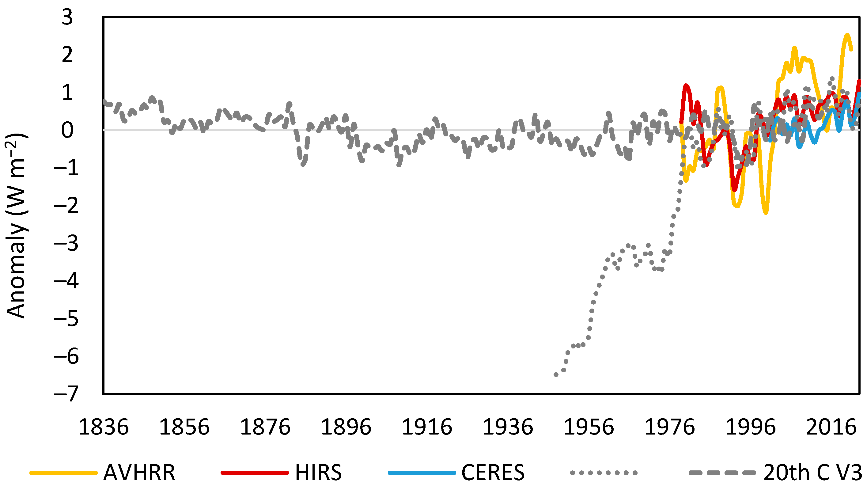
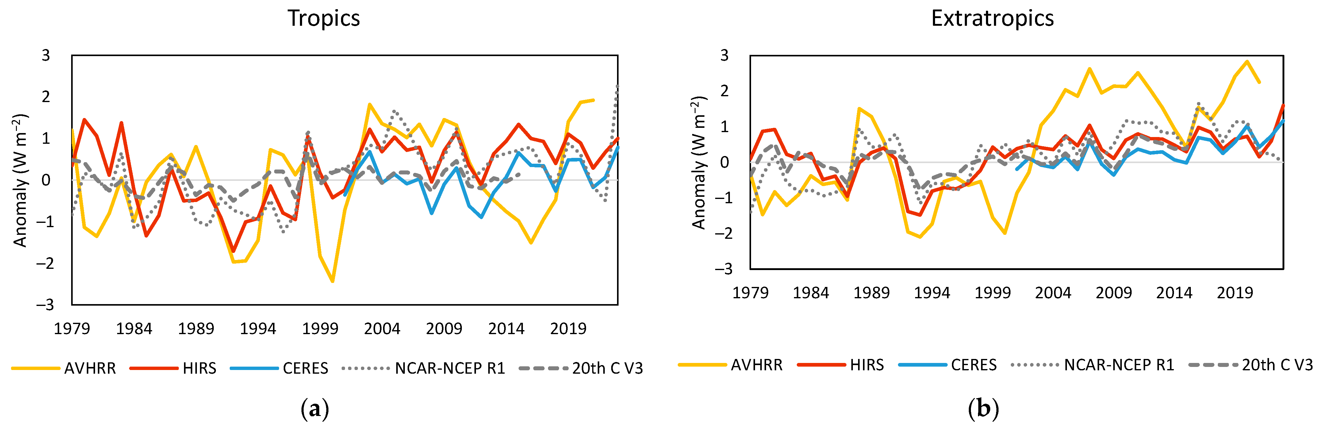
Observed OLR detected via satellite spectrometry contains regime changes (Section 3.1) but the different records are not closely aligned in the way that temperatures are [19,23]. HIRS samples more of the atmospheric column than AVHRR and is more highly correlated with reanalysis data. The similarly correlated CERES record has the disadvantage of being half its length.

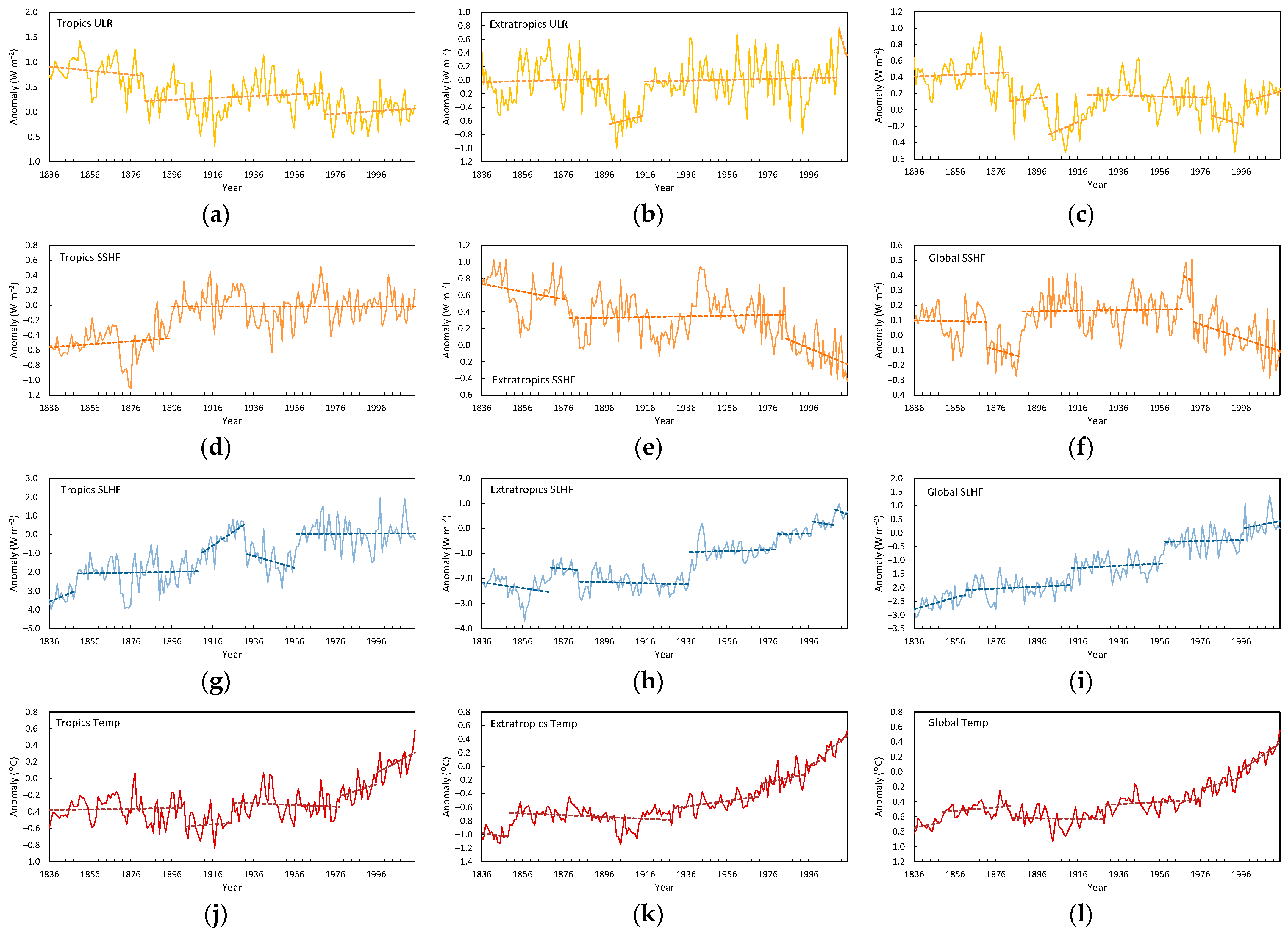
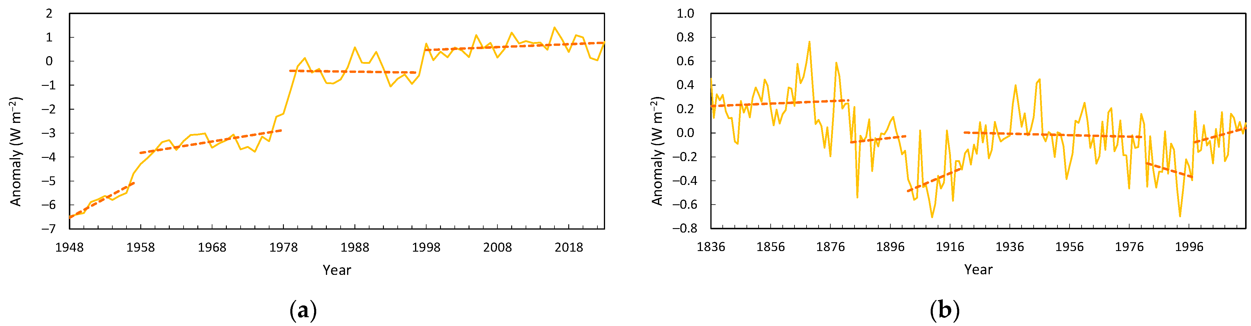
Reanalysis data also showed shifts in OLR, but they were less reliable than observations. Surface energy fluxes and temperature analyses in the V3 reanalysis (1836–2015) also contained multiple shifts (Section 3.1.2). Model reanalyses are currently not considered as reliable references for global energy balance [80]. Climate models also revealed regime shifts in both surface and TOA flux data (Section 3.2.1, Figure 8). Regime shifts are, therefore, an inherent aspect of radiative flux data in observations, the reanalysis model and climate model behavior, regardless of their accuracy.

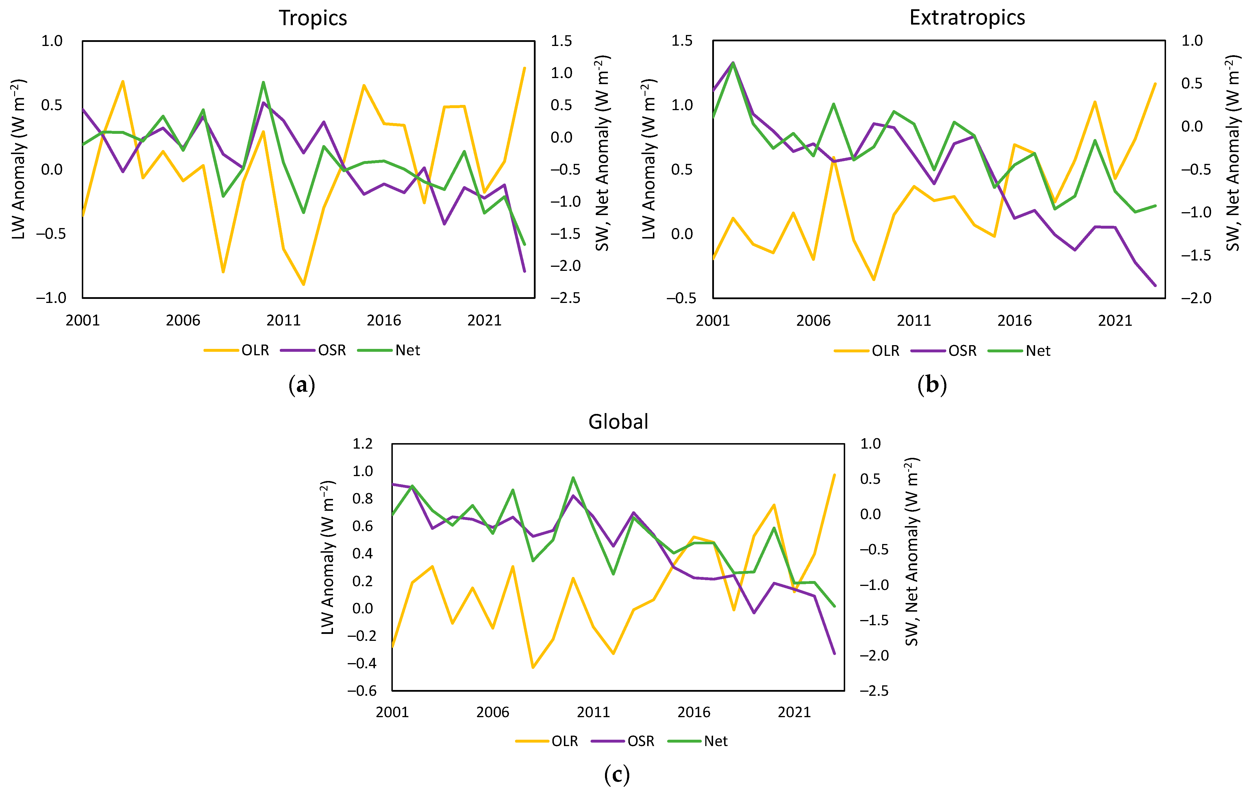
The relationships between OLR, OSR and Net were investigated for both CERES observations and CMIP5 model data. The CERES EBAF-TOA Ed-4.2.1 record 2001–2023 registered shifts in all three variables. Nonlinear behavior was identified, but the record was too short to conclude whether these constituted steady-state regimes.

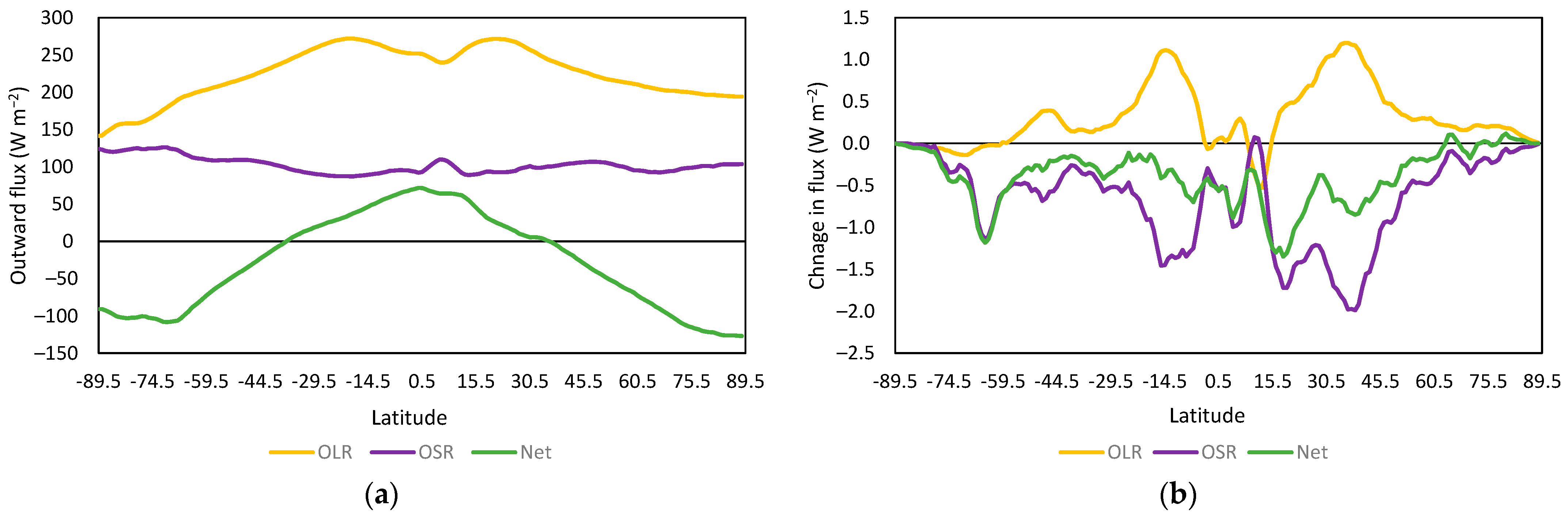
The complementarity between the three variables in both records was notable. Both annual timeseries (Figure 6) and latitudinal data at 1° resolution (Figure 7) from the CERES data showed significant complementarity between OLR, OSR and Net. For the raw data, OSR and Net were most closely aligned, especially in the NH and OLR–OSR N of 30° S. For stationary data, the OLR–OSR relationship was strongest in the NH, OLR–Net in the SH and OSR–Net globally. Most of the change signal was due to changing cloud effects, attributable to rapid increases in SST.

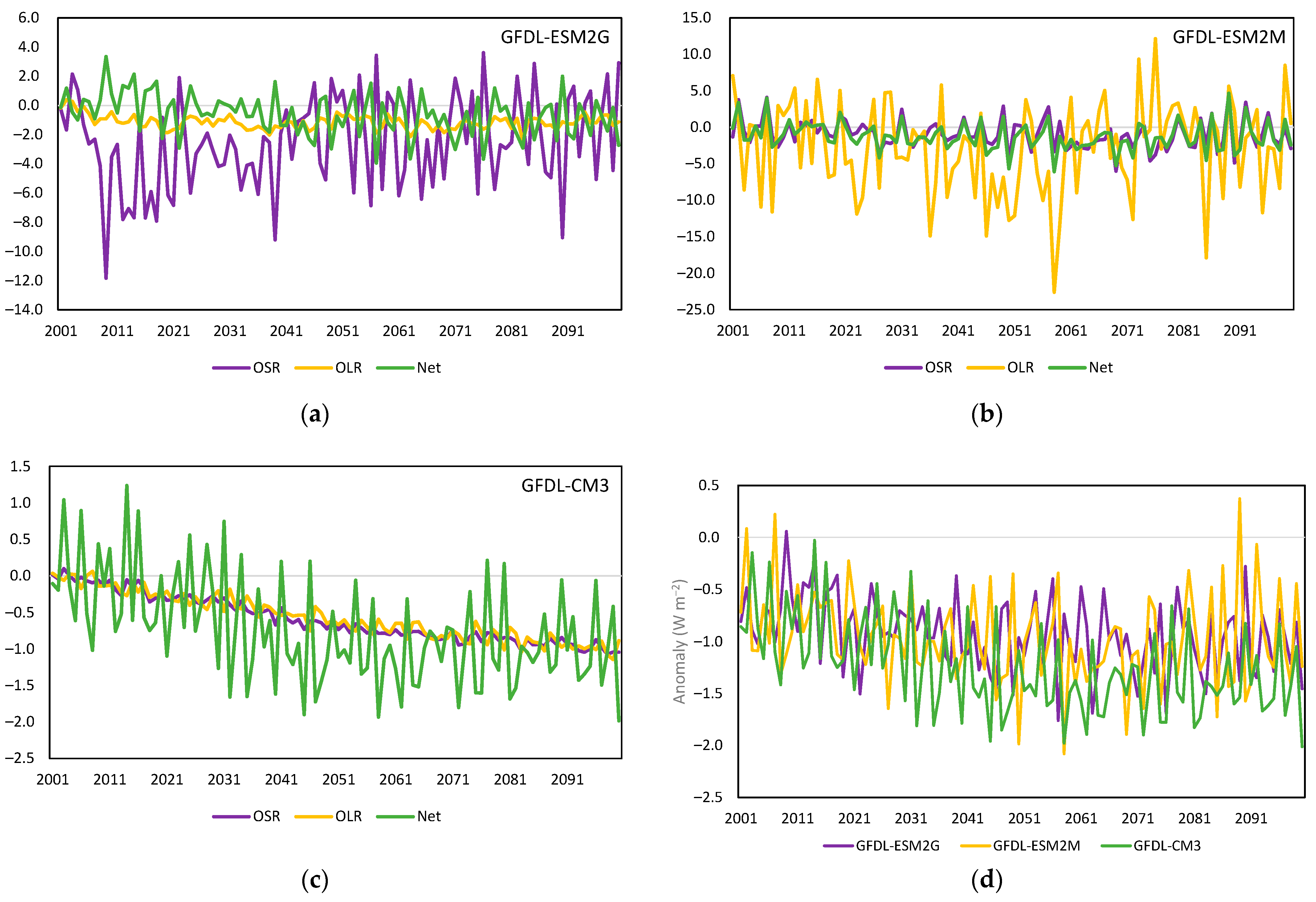
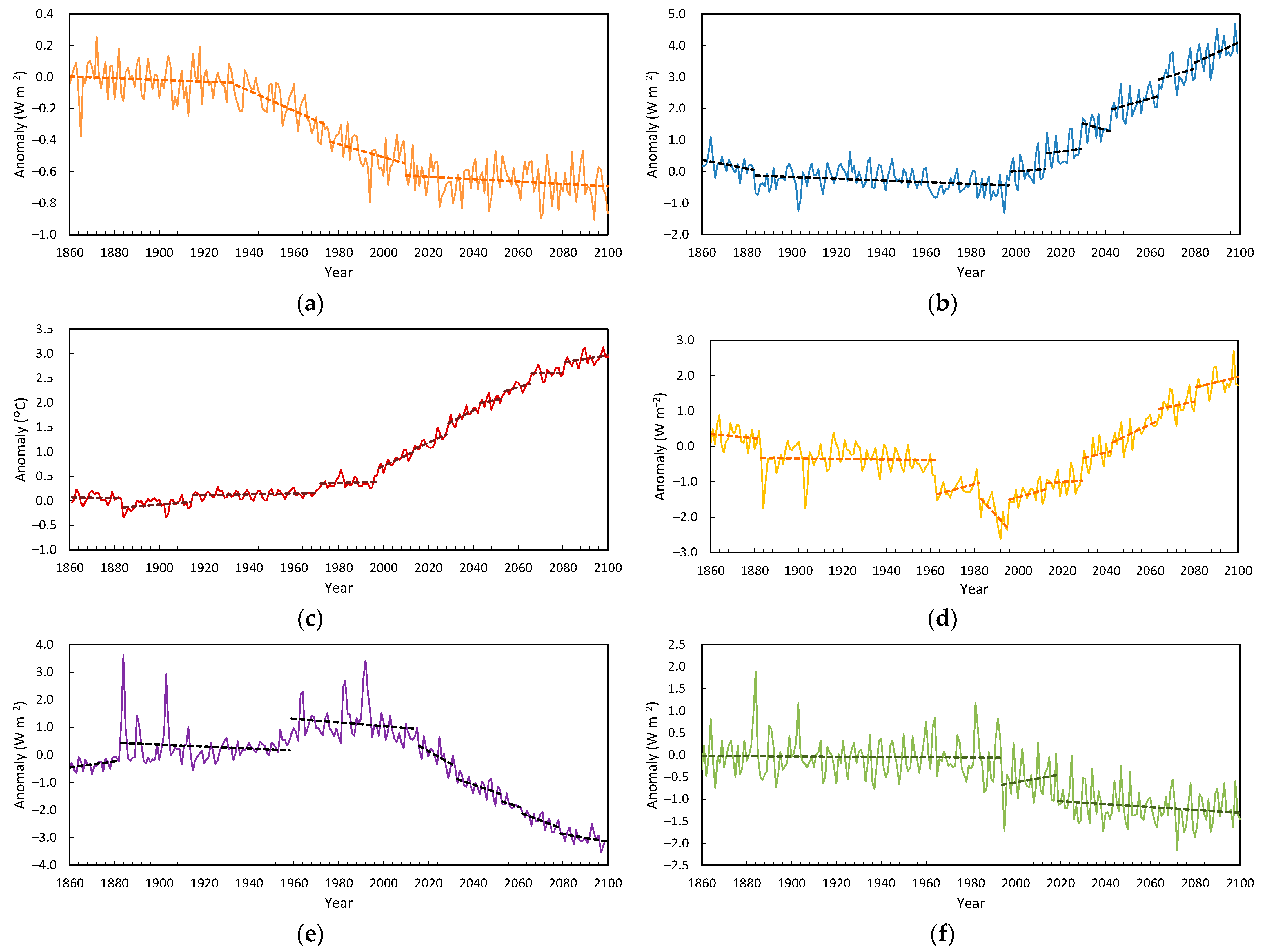
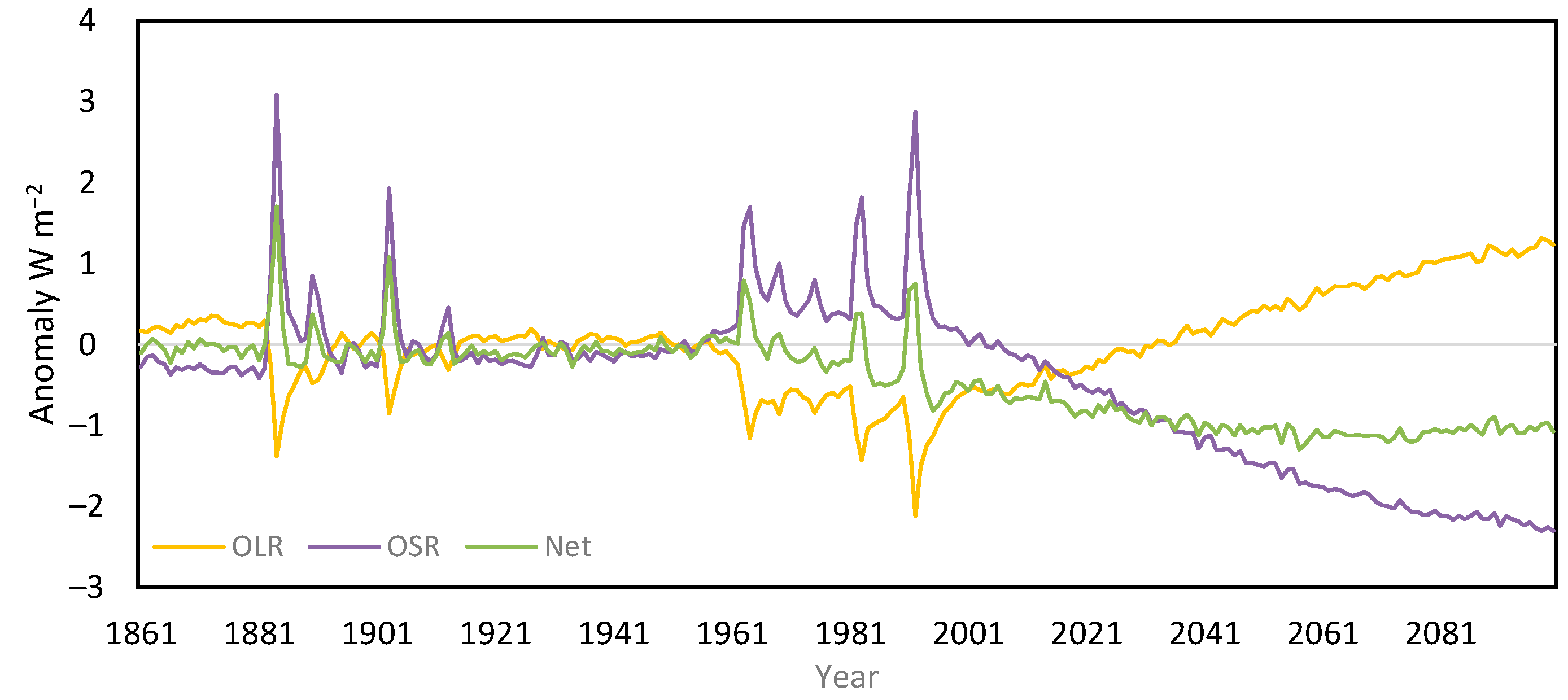
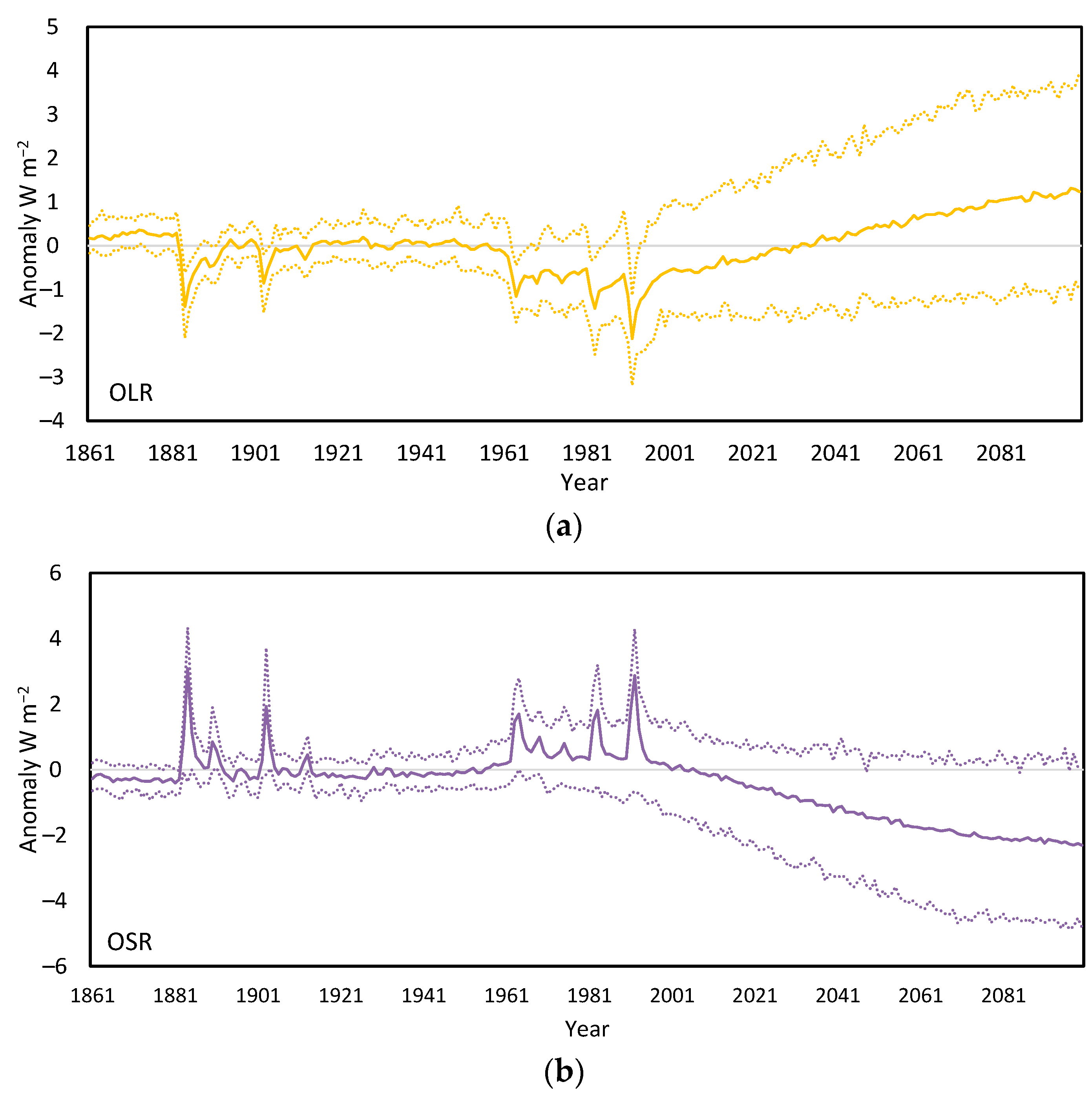
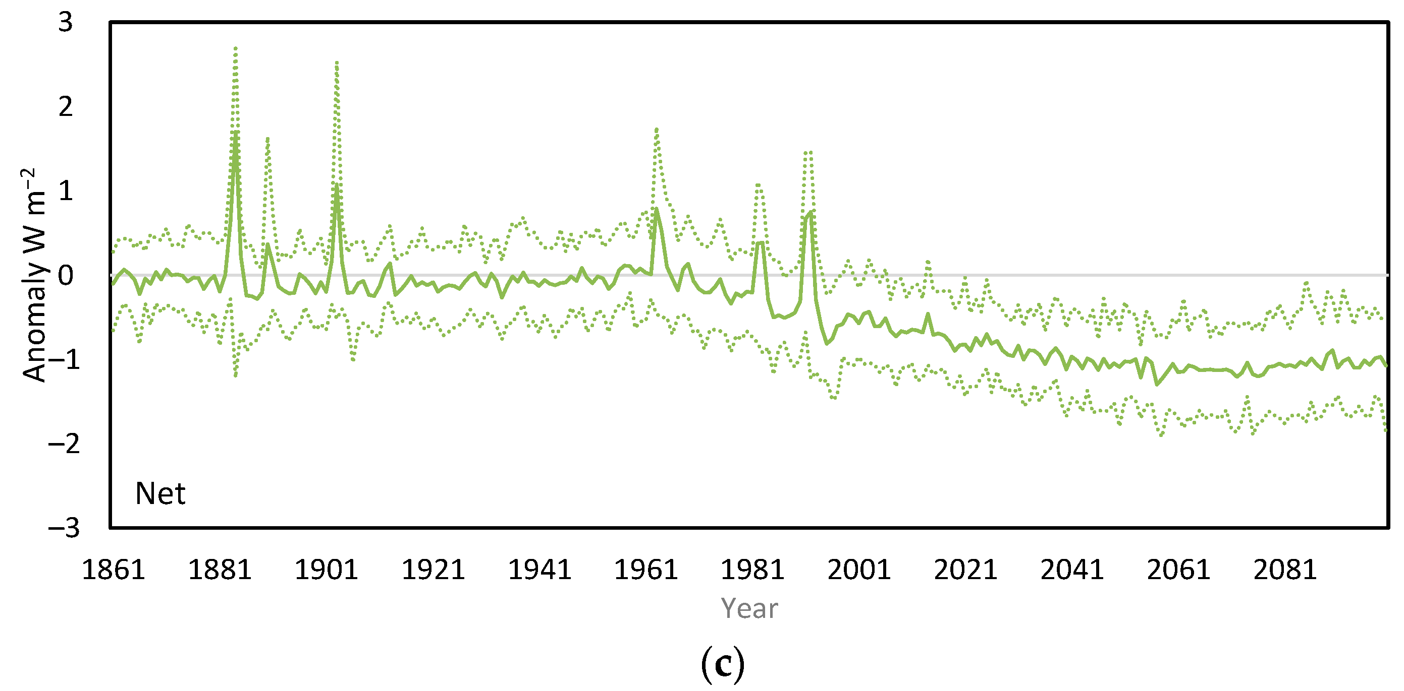
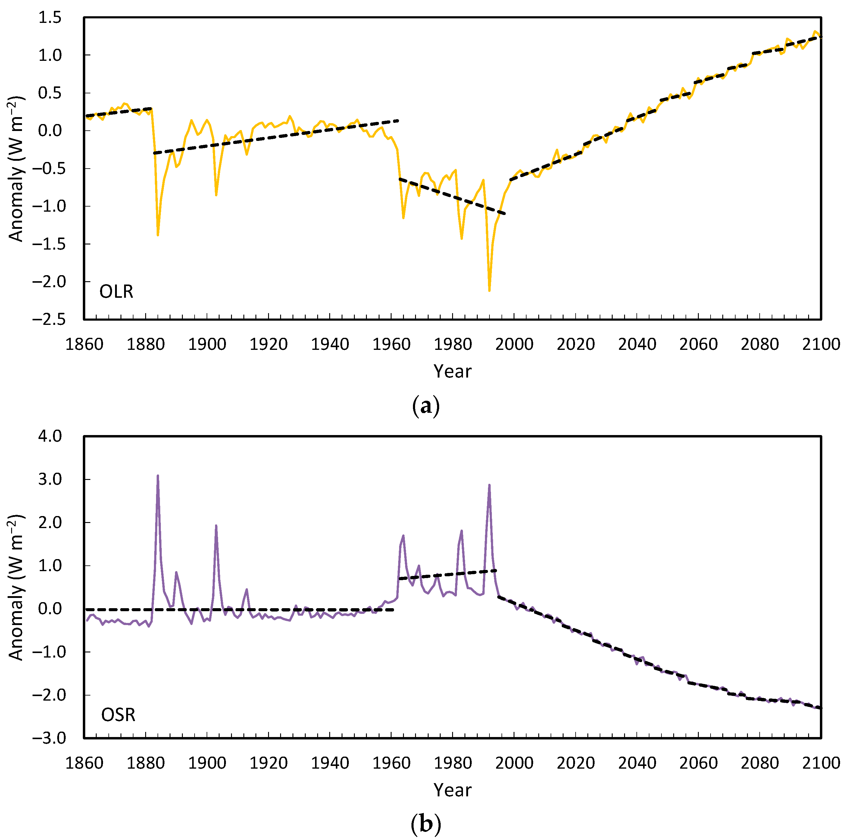
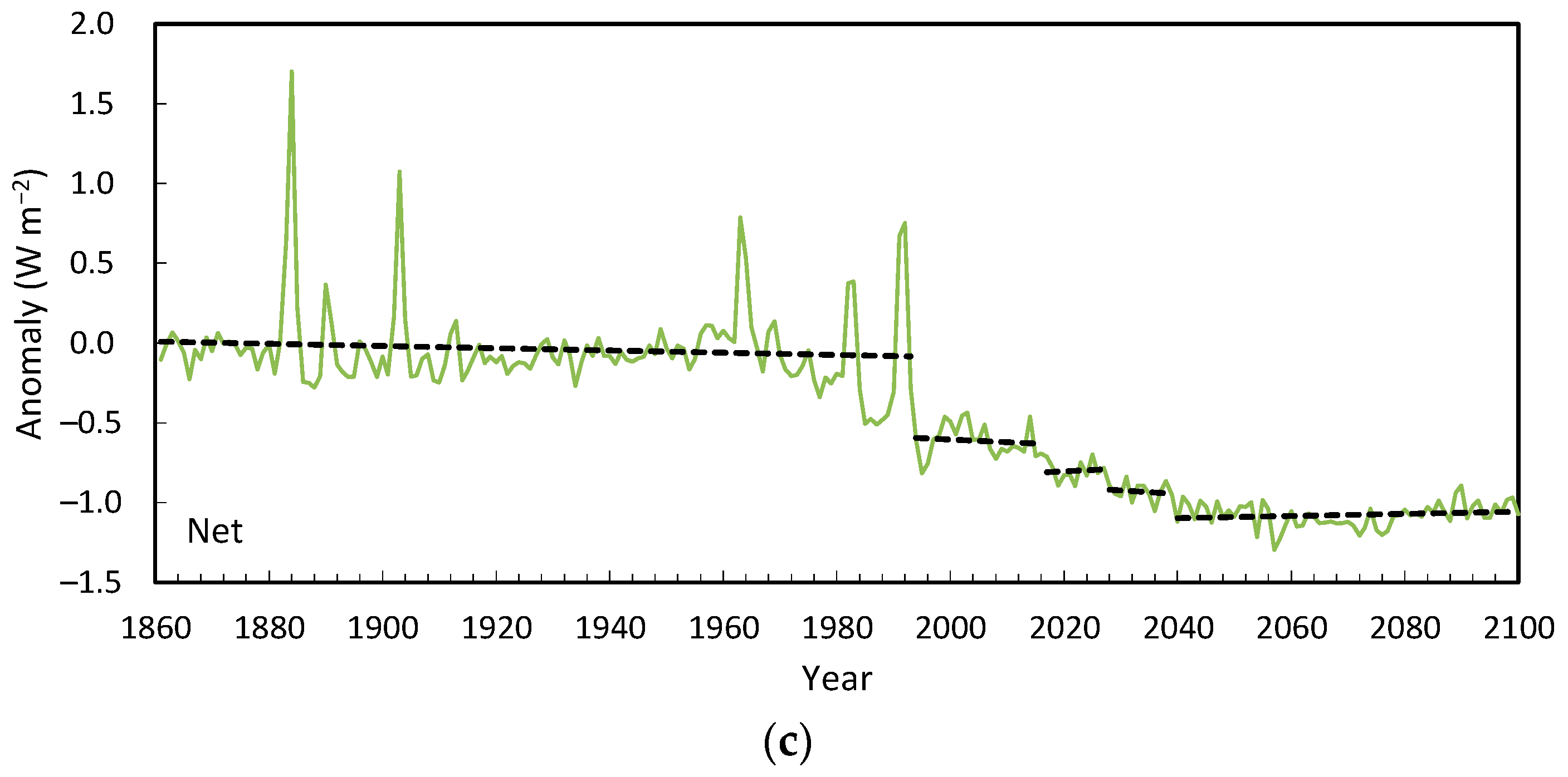
Models from the CMIP5 historical and RCP4.5 ensemble exhibited stable regimes in OLR and OSR during the historical period, but during the 21st century, both records became more trend-like. Net was extremely stable over time for 26 of 27 models tested, due to OLR and OSR compensating for each other. The range of uncertainty for Net in 2100 was about 25% of that for OLR and OSR.

The ensemble members (26/27) maintained equilibrium until 1963–1995, undergoing one to three shifts, with all but one stabilizing by 2039. Most of the initial shifts were triggered by volcanic forcing. The ensemble average for Net showed three distinct shifts, whereas those for OSR and OLR in the 21st century were dominated by trends. The preservation of shifts in an ensemble average when both its inputs show gradual change is overwhelming evidence for self-regulation.

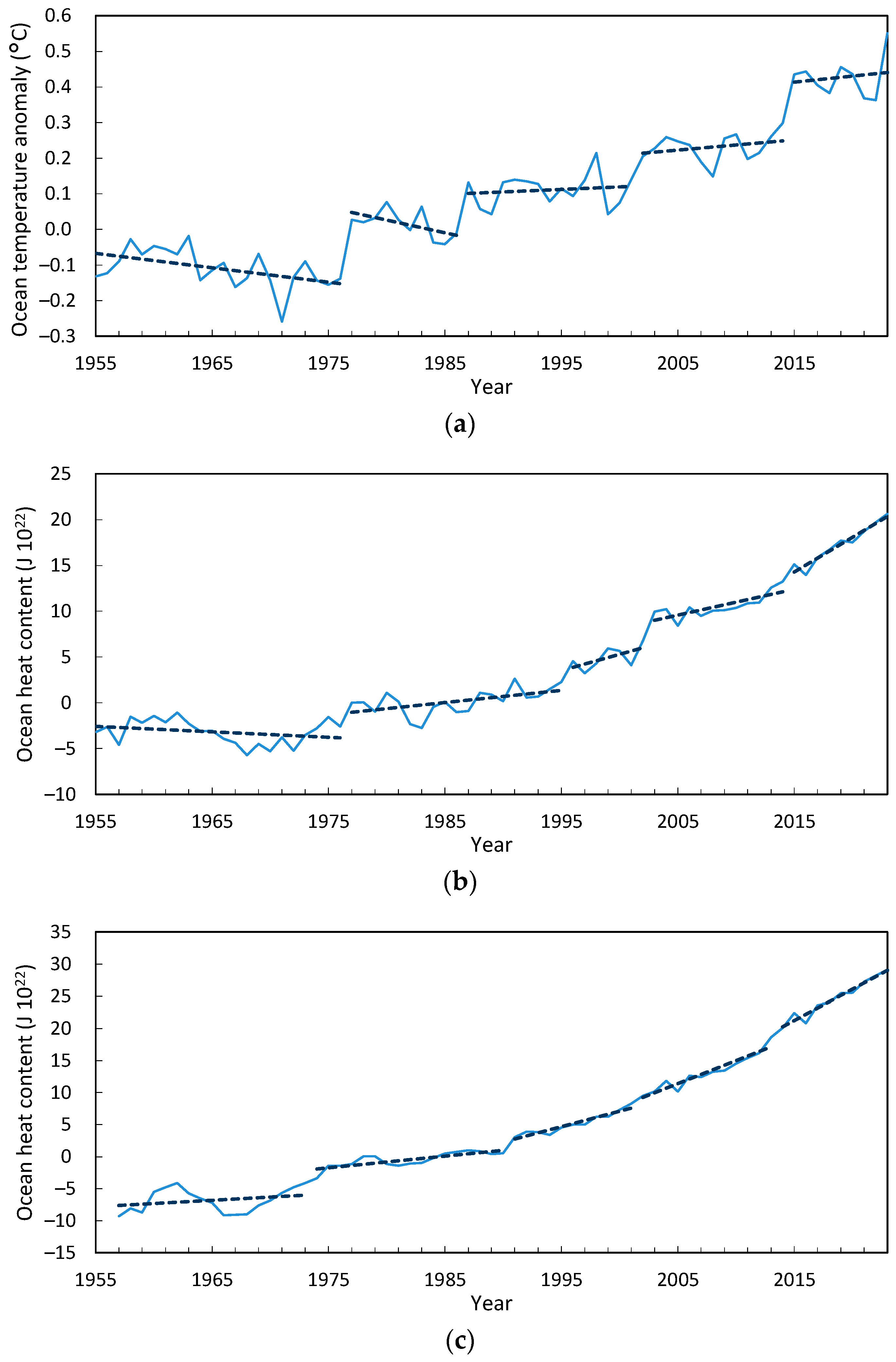
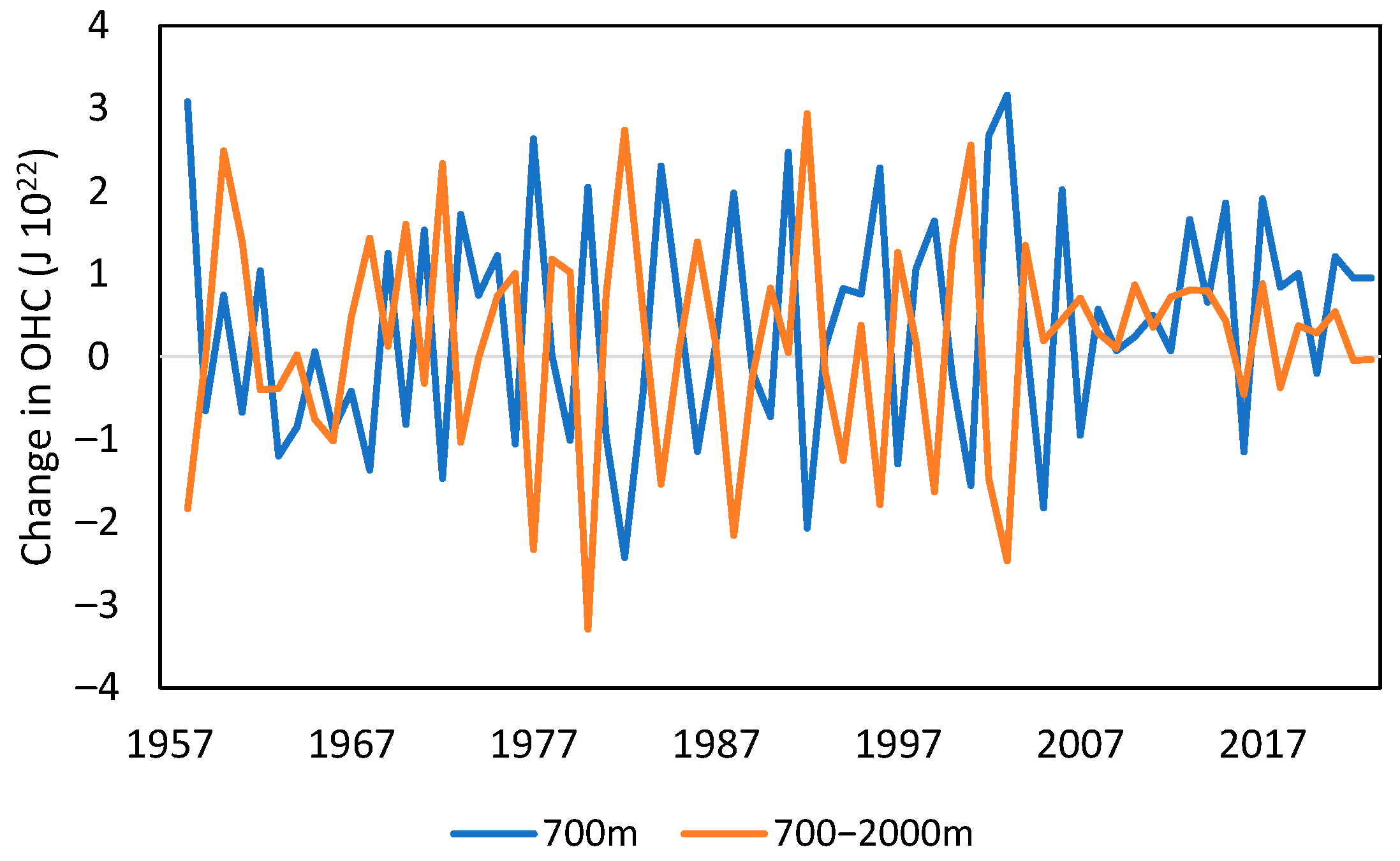
Changes in EEI as reflected in OHC were also more complex than generally assumed (Section 3.1.3, Figure 6). Three layers, 100 m, 700 m and 2000 m, were analyzed for regime shifts. These constitute around 89% of the additional heat imbalance [11,81]. The top 100 m of the ocean contains roughly 34 times the total heat in the atmosphere and is strongly regime-like (Figure 6a). Since 1957, the upper 700 m has accumulated 23 × 10²² J to 2023 and the 1300 m beneath, another 8 × 10²² J. The rate of accumulation in each has increased only slightly over that time.

However, that heat is not gradually percolating downwards. Year-on-year changes between the upper 700 m and lower 1300 m are inversely correlated (−0.67). The lower layer influences the layer above from year 2–9 at p < 0.05, through oscillations that peak in lag-years 2 and 4–5. The only other interaction of note is between the 700 m and 100 m layers, also oscillatory. This implies that the deeper ocean is acting as a dynamic buffer, with oscillations extending vertically from the depths to the surface. Changes in the 100 m layer are uncorrelated with the other two. Note that the strength of interannual characteristics changes from 2005 due to an expansion of the observation network, which may modify these conclusions, but the overall pattern is robust.

These complex behaviors extend from the deep ocean to the top of atmosphere. They do not support the gradual change imposed by the standard model. This suggests a more complex thermodynamic response to forcing than currently assumed.

4.2. A Complex Thermodynamic Response to Energy Imbalance

The standard thermodynamic view of Earth’s climate is of a single heat engine driven by solar radiation. It is based on the behavior of a classical heat engine, which begins with the idealized, perfect (Carnot) heat engine, modifying it to account for real-world processes such as friction. Driven by increasing heat, the engine will run hotter until it reaches a balance with its external environment, consistent with Equation (1). However, this structure is too simple to produce the results described here.

In classical thermodynamics, the experimenter provides the engine and focuses on its interior behavior, usually beginning with an ideal gas. In a natural system such as climate, where gas, liquid and solids exchange different forms of energy, both the engine and its behavior have evolved within a set of thermodynamic constraints. Any complexity produced is emergent. The differences between these two cases and a summary of the constraints facing the natural heat engine are outlined in Appendix B.2.

These evolutionary processes have produced a complex set of natural heat engines, all open. The main two are the radiative and dissipative engines. The radiative engine represents radiative exchange between Earth and space, and the dissipative engine is nested within that. They share the conservation of energy, but the dissipative heat engine also conserves mass and angular momentum [82,83,84].

The radiative engine is governed by the physics of radiative transfer, the amount of which constrains the dissipative engine. The upper boundary of the radiative heat engine is the nominal top of the atmosphere where the difference between incoming and outgoing radiation is at a minimum (zero if at equilibrium). Due to different heights of emission, this boundary is highly attenuated; for satellite measurements, a height of 20 km has been chosen [85]. The radiative engine performs no work itself, but the dissipative engine does. This raises the question as to whether the top of the atmosphere forms a strong enough boundary for EEI TOA to be considered as a climate driver, or whether the internal energy imbalance within the dissipative engine is what matters most.

The upper boundary of the dissipative heat engine is constrained by meridional heat transport, i.e., mass transport described by general circulation. To maintain equal amounts of energy loss from both hemispheres, ocean and atmospheric heat transport compensate for each other latitudinally [86,87]. Within this limit, modeled variations in total heat transport between glacial maximum and 4 × CO₂ climates vary by only 2% [88]. The lower boundary of the dissipative engine intersects with land, the biosphere and deep ocean—interacting with earth system processes that exchange energy on longer timescales [84,89].

The two have different energy profiles. For the radiative engine, incoming solar radiation averages 340 W m⁻² and net surface radiation is 104 W m⁻² [90]. The boundary between the two engines is complex, taking place at different altitudes, latitudes and seasonally, so the 104 W m⁻² is nominal.

The dissipative heat engine is a far from equilibrium chaotic system [89,91,92,93,94], whose complexity arises from the interplay of positive and negative feedbacks, instabilities and saturation mechanisms [95]. Like any flow system, it is restricted by its narrowest point, which is the maximum available power for meridional transport of heat from regions of excess to the higher latitudes.

Kleidon [84] estimated the global average heat transport to be 48 W m⁻² with a mean rates of power generation of around 2 W m⁻¹ in the atmosphere and 1 mW m⁻² in the ocean. This is consistent available potential energy as conceptualized by Lorenz [96,97] and quantified by Oort [98]. It makes up about 2% of net surface radiation (104 W m⁻² [90], consistent with estimates from reanalyses [99]. The Lorenz model separates kinetic energy into overturning (or zonal) and eddy kinetic energy. Measurements of each show that the power generated during overturning processes is largely cancelled out while the eddy (meridional) power is retained [100].

From an engineering perspective, a 2% efficiency rate is very low, but from an ecological perspective, the dissipative heat engine is very efficient. It has evolved in such a way to use the momentum from rotation, tidal effects, gravity and energy flows from friction, the biosphere and the hydrosphere to maintain climate in steady state, achieving a lot with very little. This is maximum flow efficiency, moving the greatest possible mass with the least resistance while expending all available energy [101].

A key justification for the standard model is that the single heat engine is close to thermodynamic equilibrium. This assumption is based on the energy profile of the radiative engine. The estimated historical ERF of 2.72 ± 0.76 W m⁻² in 2019 [8] is 0.8% of incoming solar radiation (340 W m⁻²). This is small. However, the radiative engine performs no work.

Historical ERF exceeds the maximum power limit of the dissipative heat engine (~2 W m⁻²), which performs all the work. Adjusted EEI TOA from CERES 2012–2023 is 1.09 ± 0.11 W m⁻², over half this power limit. Because it can only change marginally, this maximum power limit acts as a choke point.

The close-to-equilibrium argument is used to justify the application of the fluctuation–dissipation theorem [95,102,103]. Linear response theory holds that the response to an external perturbation is expressed in terms of the fluctuations of a system in thermal equilibrium [104]; i.e., the responses to small external and internal perturbations are identical. The main application of this theory is in the use of the signal-to-noise model.

However, when forcing produces a nonlinear response, Ruelle’s [105] requirements for the fluctuation–dissipation theorem to hold, fails: “for a small periodic perturbation of the system, the amplitude of the linear response is arbitrarily large”. This is an appropriate description for forced regime shifts in the dissipative heat engine. In mathematical terms, the response is inhomogeneous as a function of time.

The radiative and dissipative engines also have different relationships with entropy. Entropy can be addressed in two ways: entropy generation through thermodynamic processes and entropy as a state variable. The Clausius definition for entropy production is the amount of heat unavailable for work. The Boltzmann–Gibbs definition is the number of microstates available to a macrostate [106,107]. Entropy production within climate has been characterized as internal and external [108,109,110], which aligns with the radiative and diffusive engines. For Boltzmann–Gibbs entropy, a nonequilibrium dissipative system will evolve towards its maximum entropy at steady state.

Regarding external entropy production, the conversion of incoming shortwave solar radiation to outgoing shortwave scattered and longwave radiation increases the entropy of the universe [84,110]. A warming climate, therefore, increases external entropy.

In the dissipative engine, steady-state entropy decreases with warming. This does not violate the second law because the engine is open and external entropy is increasing. The preindustrial climate, with its capacity to shift both warmer and cooler, had higher entropy than today’s climate, which can access fewer microstates because it is being forced in one direction. Forcing decreases the internal entropy of the climate system because it becomes more organized. Because the dissipative system is already at its maximum flow efficiency, any response to forcing requires a change in dissipation modes within the maximum power limit.

Shifting to a warmer climate incurs a cost that results in greater irreversibility, sometimes referred to as irreversible entropy [111]. Internal entropy production is better viewed collectively as resistance, which is subject to conservation laws. This includes the irreversible entropy associated with friction and the hydrological cycle [112,113,114]. Because meridional heat transport is fixed, increases in dissipation need to switch from low energy density–low resistance modes, to higher energy-density pathways with greater resistance (e.g., from the ocean to the atmosphere and from dry to moist atmospheric transport). The estimated power limit for large-scale convection is 2 W m⁻²; for dry convection and sensible heat flux from land, it is 4 W m⁻², and for moist convection, it is 7 W m⁻² (data from Kleidon [84]).

Constrained by the additional 5 W m⁻² cost that accompanies moist convection, only 2–3% moisture per °C of warming being is added to the observed climate, rather than the potential 7% estimated by the Clausius–Clapeyron relationship [115,116]. Self-regulation requires a balancing act between all of these processes. These trade-offs dictate the transient warming rate, not the rate of ocean heat uptake efficiency. The latter is an intermodel uncertainty, not a real-world constraint.

In shifting to warmer dissipation modes, climate is compelled to accommodate higher levels of irreversibility. This acts as a drag on the system. It is similar to the metabolic adjustments biological systems have to make in order to maintain elevated levels of dissipation [117].

4.3. EEI and Self-Regulation

OLR and OSR are generated by two different energy pathways, so the complementary relationship between the two in conserving total energy can only be achieved through self-regulation, where a change in one is compensated by the other in maintaining EEI TOA in a given state. Even though the presence of steady-state regimes in EEI TOA could not be confirmed for observations, the strong model consensus is a robust result.

The presence of steady state regimes has been confirmed for air temperature, atmospheric moisture and OLR (observations and models); surface fluxes (reanalyses and models); shallow ocean temperatures (observations); and OSR and Net (models). Other forms of self-regulation are interhemispheric exchange to balance outgoing energy and the relationship between OSR and OLR in maintaining that balance in net spatially and temporally. A further possibility involves EEI, where the oscillating nature of heat build-up between the mid-level ocean (to 700 m) and deeper ocean suggests that active connections exist between the deeper ocean and top of the atmosphere.

The trade-off between OLR and OSR in maintaining Net indicates additional self-regulation that is not immediately apparent, namely, spatial regulation within the climate network. Feedback effects from surface warming vary widely, especially over the ocean, ranging from strongly positive to neutral-negative. Locations where regime shifts are strongest can, therefore, influence warming rates and patterns, influencing the relative contributions of OLR and OSR. Appendix B.2 contains a mini review of these effects, including evidence drawn from this study.

Recent observations show that the response in EEI TOA is dominated by reduced OSR (increased absorbed shortwave radiation) due to cloud feedback, rather than increases in OLR. OLR is a product of mass transport, so it comes at a cost. The locations of greatest increase in OLR in Figure 5b are convective rather than meridional. The same processes leading to increased OLR also lead to greater moisture transport, providing the potential to change cloud characteristics, resulting in the strong complementarity between OLR and OSR.

Therefore, even though moisture increases come at the cost of greater irreversibility, cloud feedbacks provide the additional capacity to absorb shortwave radiation as a bonus. This is mainly driven by changing cloud amounts, especially low-to-mid cloud [57], with the resulting feedback dominating the amount of realized warming. Therefore, the Planck response increasing OLR and feedback manipulating OLR are coupled.

These changes involve the self-regulation of patterns of change in SST influencing cloud amounts and cloud type [57], reflected in levels of sensitivity and OSR. This is the most unexpected finding of the project. The idea that cloud amounts and characteristics can be manipulated to counterbalance OLR and OSR in order to stabilize Net is radical. However, models achieve this even when their estimates of OLR and OSR are wildly wrong (Figure A2), showing how strongly boundary conditions and system limits influence both model and real-world performance.

The dissipative heat engine regulates two types of equilibrium:

• Internal equilibrium within the dissipative heat engine, where a steady state between the coupled ocean and atmosphere is maintained at the maximum possible entropy subject to the amount of forcing. This state is buffered within critical limits.
• External equilibrium/disequilibrium expressed as EEI TOA (Net). This also is maintained in steady state, but if the accumulation rate of heat within the climate system exceeds the transient warming rate, EEI TOA can shift further negative.

In relieving forcing pressure, warming provides a negative feedback, whereas a larger deficit in EEI TOA provides a positive feedback. With sufficient forcing (e.g., RCP8.5), shifts in temperature become so frequent they merge into a curve [19]. These shifts act as gear changes. Shifts in dissipation rates cause the engine to run ‘richer’, with greater energy density and irreversibility, reducing steady-state entropy. Shifts in EEI TOA represent the inability for that warming to relieve the increasing internal energy imbalance, showing the limits of self-regulation. EEI TOA does not represent a physical limit in itself but reflects the status of the system in managing internal energy imbalance, measuring the difference between demand to return to equilibrium and supply of response within its different constraints. The oscillating relationship between the mid-level and deep ocean OHC suggests self-regulation within the climate system is four-dimensional, comprised of three spatial dimensions and one of time.

The tension between decreasing entropy within the dissipative heat engine as it warms and increasing entropy in its radiative output is similar to that nominated by Schrödinger for biological systems [118,119]. The capacity to self-regulate between the material and radiative aspects of climate to main steady-state regimes mirrors the metabolic characteristics of biological systems that utilize biochemistry. This suggests the evolutionary processes behind the development of complex natural phenomena such as the climate system precede those associated with living systems.

5. Conclusions

The factors making up two measures of Earth’s energy imbalance, EEI TOA and excess heat uptake (EEI HC), exhibit nonlinear responses to forcing over decadal timescales. Increasing radiative forcing does not produce gradual changes in EEI TOA and surface temperature. Instead, steady-state regimes emerge. Increasing excess heat does not simply percolate from the shallow into the deep ocean but forms strong regimes in the top 100 m (roughly one-third of the total) and oscillates between the 700 m layer and the 1300 m below. The two main inputs to Net, OLR and OSR, also show strong self-regulating behavior, spatially and temporally.

These behaviors are inconsistent with the idea of a passive climate being driven wherever forcing takes it. The standard thermodynamic model, representing Earth’s climate as a single, planetary-scale heat engine, cannot produce such responses.

Instead, we propose a more complex arrangement of naturally evolved heat engines. Considering climate as a dissipative heat engine coupled to a radiative engine, EEI is an emergent property of the dissipative heat engine, serving as a dynamic boundary. The dissipative engine is a far-from-equilibrium natural engine that has evolved to take the path of least resistance while utilizing its maximum power limit (2 W m⁻²). It is open to the radiative engine, receiving solar radiation and emitting scattered shortwave and longwave radiation. Net TOA, whether in balance or not, is a measure of that output.

Self-regulation is an emergent function of atmosphere–ocean coupling. The dissipative heat engine conserves energy, mass and angular momentum in maintaining a steady state. Warming acts as a brake [120], because shifting to a warmer steady state involves paying a price in terms of greater resistance (irreversibility) in order to accommodate the transport of heat with greater energy rate density. Warmer states have lower internal entropy than cooler states while increasing external entropy production. This balancing act allows the system to maintain out-of-equilibrium steady states while being actively forced. It can be viewed as a kind of thermodynamic metabolism.

The dissipative engine potentially switches through gears as energy imbalance increases. Using EEI TOA from CMIP5 models as a guide, the engine may have remained in neutral until well into the 20th century, shifted into first gear as an energy deficit emerged in the 1970s and, possibly, shifted into second gear from 2014 to 2015. Spatial patterns of surface temperature, cloud feedback effects and overall radiative (im)balance play an important part how the dissipative heat engine responds to forcing.

This nonlinear behavior also poses considerable risks, due to rapidly changing climate impacts that need to be understood and managed [21,22,121,122]. Developing predictive and diagnostic tools to better understand and manage nonlinear change is urgent and essential.