Article

Cyclic Interannual Variation in Monsoon Onset and Rainfall in South Central Arizona, USA

by
Frank W. Reichenbacher
1,* and
William D. Peachey
2
1
Desert Laboratory on Tumamoc Hill, University of Arizona, 1675 W Anklam Rd., Tucson, AZ 85745, USA
2
Sonoran Science Solutions, 550 N. Avenida Venado, Tucson, AZ 85748, USA
*
Author to whom correspondence should be addressed.
Climate 2025, 13(4), 75; https://doi.org/10.3390/cli13040075
Submission received: 26 February 2025 / Revised: 27 March 2025 / Accepted: 30 March 2025 / Published: 6 April 2025

Abstract

:
The North American Monsoon (NAM) in southern Arizona continues to be a topic of interest to many ecologists studying the triggers and characteristics of plant growth and reproduction in relation to the onset of the monsoon. The purpose of this article is to report interannual variation in the timing of NAM onset found while researching the phenology of Saguaro cactus (Carnegiea gigantea). Using a daily rainfall dataset from 33 stations located in Pima and Pinal Counties, Arizona, from 1990–2022, we analyzed monsoon onset, monsoon precipitation, annual precipitation, and the proportion of annual station precipitation received during the monsoon season. Onset was measured by the first day from 1 June to 30 September with precipitation ≥ 10 mm counted from the day of the vernal equinox of the year. Generalized Additive Models (GAMs) identified sinusoidal waves with a period of 8.6 years and amplitudes of 14–29 days, providing frequency and amplitude estimates for Sinusoidal Regression Models (SRMs). Sinusoidal wave patterns found in the monsoon onset dataset are suggested in monsoon, annual, and proportion of monsoon in station-averaged annual precipitation although in and approximately mirror-image. These unexpected findings may have important implications for forecasters as well as ecologists interested in plant phenology.

1. Introduction

1.1. Saguaro Phenology

The association of plant phenological response to the annual cycle of the North American Monsoon (NAM) has been the subject of much study by plant ecologists [1,2,3], but many details are not well-characterized. Numerous plants of the Sonoran Desert of North America are partly or wholly dependent on NAM rainfall, but when does monsoon rainfall arrive at any one location? How does arrival timing vary over time and across plant generations? Or does it vary? Appearing as it does in the otherwise extremely hot summer months of June-September, the monsoon rains are vital to plant growth and reproduction [4,5,6]. One plant uniquely dependent on the monsoon is the saguaro cactus (Carnegiea gigantea) which flowers in April, produces fruits from May–June, and disperses seeds by mid-July [7,8,9]. Timing of seed dispersal anticipates the arrival of the first NAM rainfall events in July. Seed germination and seedling establishment requires sufficient NAM rainfalls to trigger germination and then provide moisture, elevated humidity, and lower temperatures to ensure seedling establishment. Seeds of the saguaro cactus apparently do not survive for more than a few weeks after dispersal [10]. Many other species produce and disperse propagules immediately prior to NAM onset. However, as far as is known, at least a portion of those seeds survive the summer and persist in the soil for at least one more season [11,12]. Saguaro synchronization of phenological events with rainfall events and extended periods of favorable climatic conditions is crucial for reproduction. Phenological synchrony with climatic cues is an area of intense ecological research [13,14,15,16].

1.2. North American Monsoon

The synoptic NAM rainfall system emerges from seasonal variations in latitudinal migrations of the Intertropical Convergence Zone (ITCZ, [17,18]). As the ITCZ migrates northward from the equator toward Central America in the northern hemisphere spring, winds along the Pacific coast of Central America and Mexico shift from westerly to southerly, transporting increasing quantities of low-level moisture north and northwest along the Mexican coast and eventually entering into Arizona [19,20]. The ITCZ linkage is a relatively recent interpretation made possible primarily through the analysis of global precipitation revealed by satellite sensors [21]. Over the past 30 years, climatologists have achieved considerable success in explaining the causes and mechanisms driving the NAM phenomenon. In particular is the North American Monsoon Experiment (NAME) project of the early 2000s [22]. In addition to compiling impressive datasets from a variety of sensor sources, the NAME researchers worked hard to resolve disagreements regarding the source(s) of NAM moisture and the role of the Gulf of California (GoC) as a mechanistic component of the NAM system [23,24].
Previous research found some indication that the onset and retreat of monsoon weather has changed, perhaps reflecting changes in the ITCZ. Arias, et al. [25] found that the NAM season has shortened due to earlier retreat while the SAM (South American Monsoon) has lengthened by a correlated amount. Ashfaq, et al. [26], using multiple regional projections, predicted broad monsoon onset delays and less overall precipitation, which, if realized, could have significant effects on saguaro phenology.

1.3. Defining Monsoon Onset

The goal of our research reported here is to determine whether saguaro reproductive phenology is synchronized with important climatic events, particularly regarding the timing of seed dispersal and the onset of the monsoon. This first required an objective determination of the date of monsoon onset for a period long enough to discern trends and patterns. We then sought monsoon onset criteria that could be identified from a daily rainfall record, available for many stations in our area from online sources, would yield a single day date, and considered the needs of the plants of the desert. Several methods for identifying monsoon onset were reviewed.
Brenner [27] noted a variety of measurements to indicate that the northward surge of the seasonal maritime airmass from GoC to Arizona has begun, including hourly observations of temperature, dew point, and pressure. In the 1980s meteorologists associated with the U.S. National Weather Forecasting Offices in Phoenix and Tucson began to rely on dew point temperature criteria [28]. Bombardi et al. [29] catalogued detection methods or criteria from 32 published references, about half of which were solely or partly based on precipitation criteria.
Bowers, et al. [30] found that precipitation amounts triggering seedling emergence in 15 perennial plant species ranged from 17–36 mm. This threshold is higher than necessary to trigger flowering in established perennial plants. Bowers and Dimmitt [2] found that a rainfall event of as little as 9 mm was sufficient to trigger flowering in triangleleaf bursage (Ambrosia deltoidea), and Bowers [8] found that as little as 5 mm of rain triggered flowering in the saguaro cactus. Therefore, for the purposes of this analysis, it was determined that the first single-day rainfall of ≥10 mm, from 1 June to 30 September, would be used. This amount is large enough to potentially trigger plant growth, and almost every weather station in the dataset recorded it on at least one day at some point during the NAM season.
As plant ecologists, we are interested in the influence of environmental signals on phenological triggers and how this might affect the viability of the saguaro cactus and many other plant species. During investigations of the relationship between saguaro phenology and climate, we found interesting patterns in NAM early and late onsets. The purpose of this article is to report the results of our preliminary analyses suggesting previously unreported cyclic interannual variation of in NAM onset and precipitation in South Central Arizona. In subsequent publications we plan to present analyses of the influence of changes in the date of onset of NAM on saguaro phenology.

2. Methods

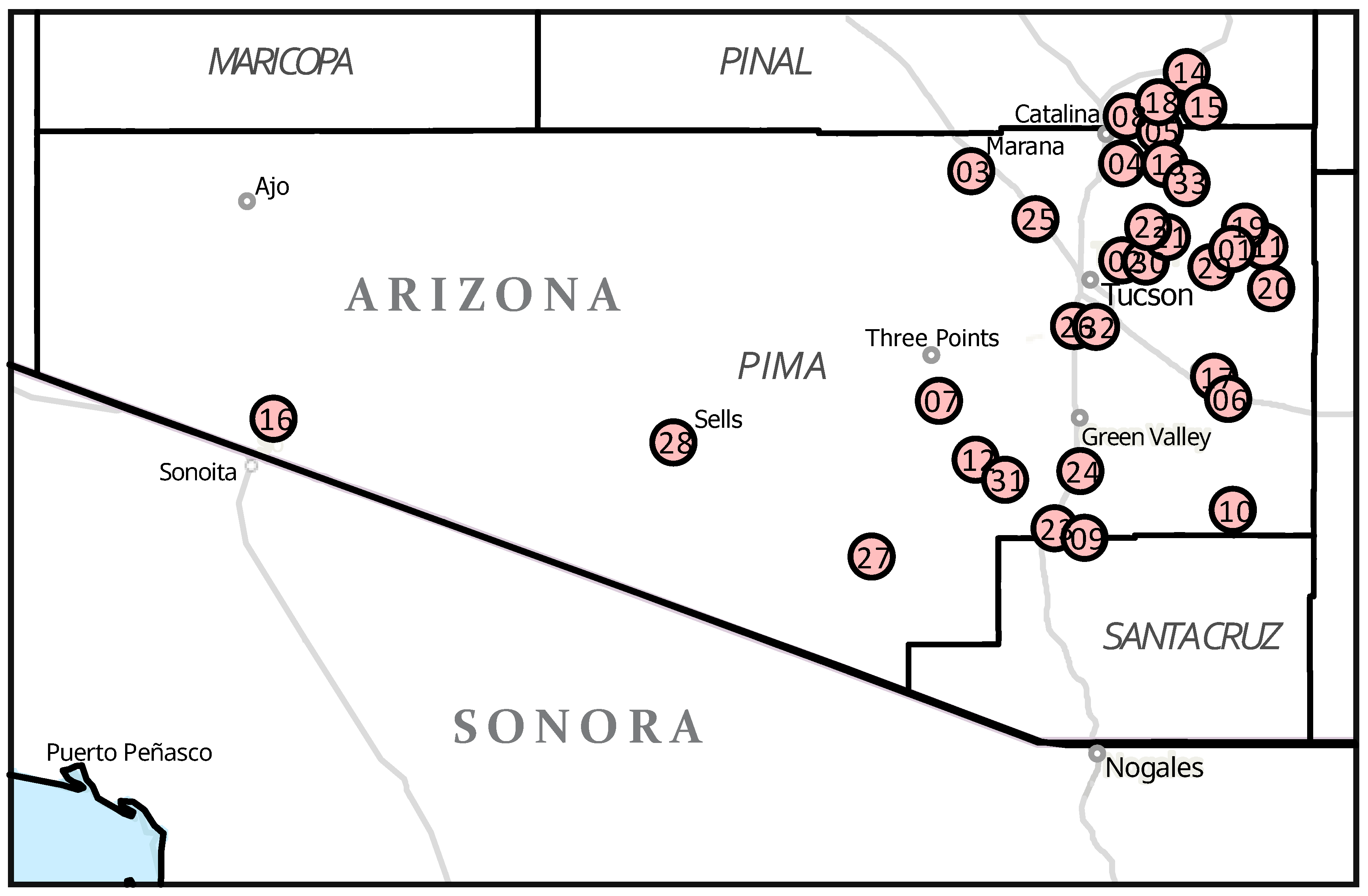
Precipitation Dataset

The monsoon season was considered to include the period from 1 June to 30 September, and monsoon onset was defined as the first day from 1 June to 30 September with single-day rainfall of ≥10 mm. Our primary dataset was constructed with daily precipitation gathered from the Pima County, Arizona, ALERT network of remote reporting rain gauges [31], the Global Historical Climatology Network (GHCN-Daily [32,33]), and Remote Automated Weather Stations (RAWS [34]), most with records from 1990–2022 (Table 1, Figure 1). Data for the full 33-year period from 1990–2022 were obtained from 22 of 33 weather stations. Years of record for the remaining 11 stations ranged from 21 to 32 years.
Variables of interest, which will be referred to as below for the remainder of this paper, extracted from the precipitation dataset included:
  • Day-of-year (DOY onset) of the first one-day rainfall events of ≥10 mm from 1 June–30 September, 1990–2022. To mitigate possible calendar bias in our method of determining the day-of year of monsoon onset, the dates of monsoon onset were counted from the date of the vernal equinox of that year instead of from the first of the year. The date of the vernal equinoxes was obtained from the seasons calculator at timeanddate.com for Tucson, Arizona [35].
  • Total monsoon rainfall (MR, mm, 1 June–30 September).
  • Total annual rainfall (AR, mm).
  • Proportion of mean annual station rainfall falling from 1 June–30 September (PAR). Each year value in this vector is calculated as the ratio of monsoon rainfall of the year and station mean annual rainfall across years.
Of the 33 stations used in the analysis, all but three were within a 65 km radius of downtown Tucson, representing 2278 m of elevation from 512 m, at the Organ Pipe Cactus National Monument Headquarters, to 2790 m at the summit of Mt. Lemmon, Santa Catalina Mts. The geographical area covered by the selected stations, 17,225 km2, was chosen mainly because of the predominance of the Pima County ALERT network in the dataset within the range of the saguaro, but with the addition of stations with sufficient periods of record to sample the region west and south of Tucson, and a few RAWS stations to fill in elevation gaps. The Spatial Autocorrelation tool in ArcGIS Pro v. 3.2 [36] was used to determine whether the 33-year station means of the day after the vernal equinox of the first-day rainfall ≥ 10 mm was influenced by proximity. The input data were weighted to include station elevation (z coordinates) calculated using inverse Euclidean distances.
When required for particular analyses, missing values were filled using the imputeTS package moving average algorithm (R package, ImputeTS [37]). On the few occasions with no rainfall ≥ 10 mm was recorded during that period (17 of 1049 DOY records), the highest one-day amount during the period was substituted. The substitution procedure may have led to a slight bias to later DOY onset as at some of these stations the highest amount recorded from 1 June–30 September occurred very late (as late as 30 September).
Least-squares linear regression models (LRMs) were created for the four variables time series listed above as well as (1) DOY onset and MR on elevation, (3–5) MR, AR, and PAR with DOY onset as predictor using base R ([38]). To investigate correlations among stations, Spearman’s Rank statistics for the 33 stations with respect to DOY onset were calculated, also in base R ([38]). Autocorrelation function plots and residuals plots were created for the DOY onset time series using the R forecast package [39]. Normality was investigated using probability density and QQ plots and Shapiro–Wilk tests of the per-station onset time series base R [38]. The time series of the four key variables listed above were tested using multivariate (multi-site) Mann–Kendall monotonic trend (R package trend, [40]). Cross-correlation tests were run with MR, AR, and PAR time series as response and DOY onset as the predictor using base R [38].
Patterns in scatterplots for each variable (DOY onset, MR, AR, PAR) suggested non-linearity that generalized additive models (GAMs) might elucidate. GAMs are widely employed in many fields when non-parametric analyses and relaxation of normality assumptions are desired [41,42,43]. Fit curves with basis dimensions set to k = 10 were generated from GAMs developed in R using the MGCV package [44] for the four variables. The results were useful in estimating sinusoidal wave periods and coefficient starting points for sinusoidal regression models (SRMs) using the MATLAB (R2024a) Curve Fitter tool [45] of the form:
f(y)=a sin(bx + c) + d
where y = DOY onset, MR, AR, or PAR, a = amplitude, x = year, b = change in period, c = horizontal shift, and d = vertical shift (calculated in base R [38]).

3. Results and Discussion

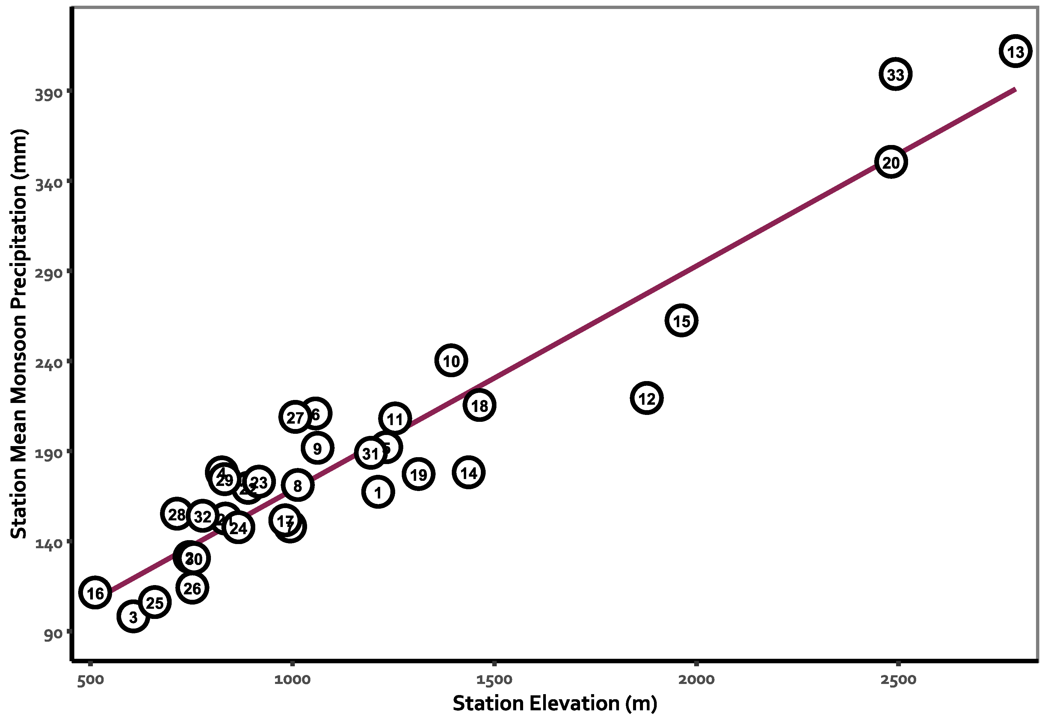
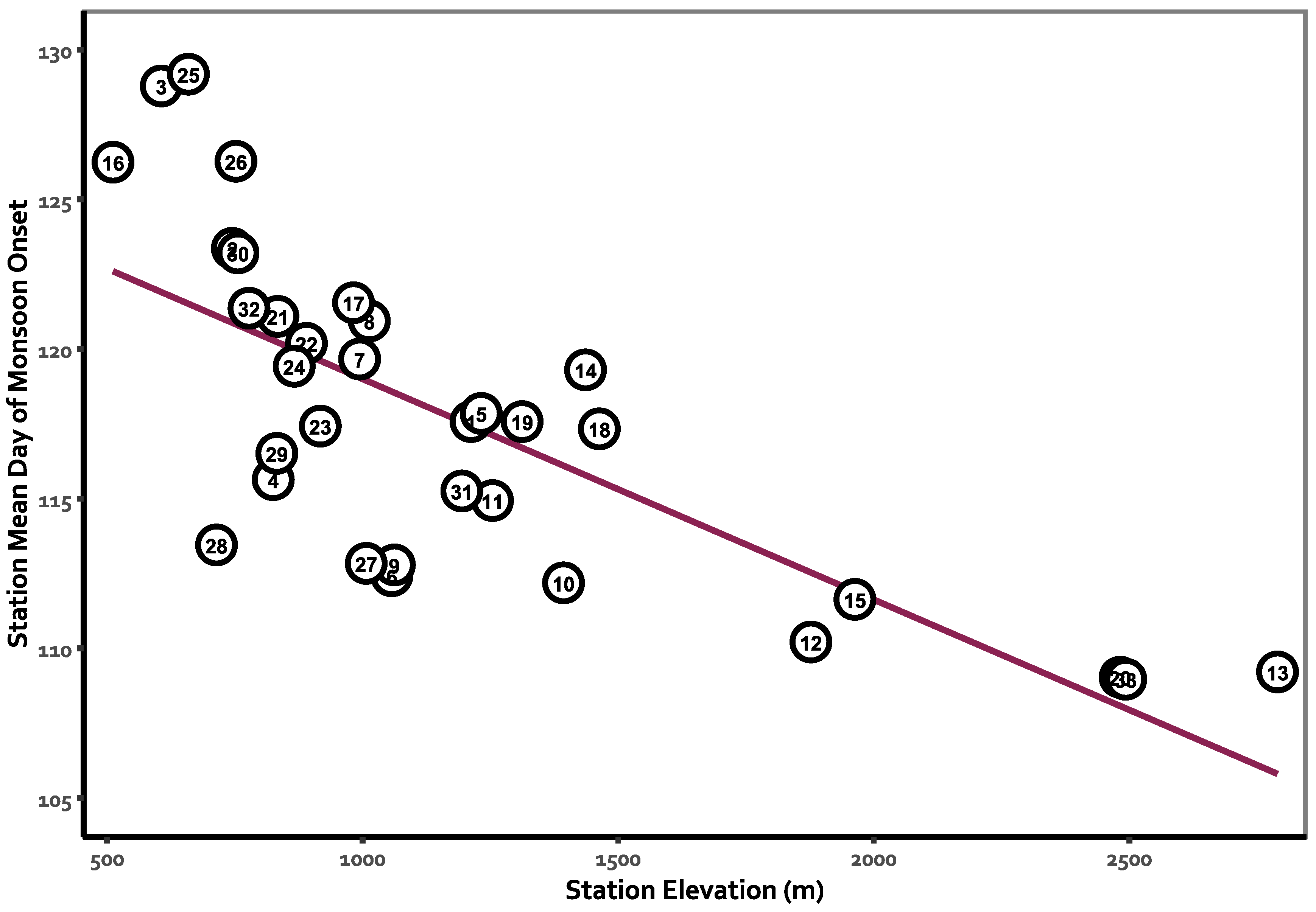
3.1. Effect of Elevation on DOY Onset and Precipitation

In our NAM study area, orography strongly influences precipitation; and at most sites, there is a significant positive relationship between monsoon precipitation and elevation [46,47]. Figure 2 illustrates this with LRM of mean station MR on station elevation (R2 = 0.891, p-value ≤ 0.001). In addition, DOY onset data regressed on elevation (Figure 3) also suggested a positive relationship (R2 = 0.540, p-value ≤ 0.001). Thus, an early onset is associated with higher MR along the elevational gradient. Higher-elevation sites generally have a greater probability of rainfall ≥ 10 mm on any day (both from the increased frequency of rainfall events and from the greater precipitation received from each event) and are, therefore, more likely to achieve our rainfall threshold (≥10 mm/day) sooner rather than later in any arbitrarily chosen period, including the monsoon season. The association of earlier onset with increasing elevation in our region is not unexpected. However, it is surprising that our DOY onset data, mixing untransformed gauge data from a broad elevational range should nevertheless exhibit the coherent cyclic pattern of interannual variation described in the next section. Early in our analysis, we removed the effects of elevation on DOY onset variance. However, this had almost no effect on subsequent analyses and was not pursued. The positive correlation between monsoon precipitation and elevation observed in our gauge ensemble was not observed in other areas, including some relatively close by, such as northwestern Mexico, where distance from the Pacific Ocean coastline and the Sierra Madre Occidental are more reliable predictors ([48,49]).

3.2. Monsoon Day-of-Year Onset

Table 2 lists the 33 weather stations, mean DOY onset, MR, AR, and PAR for each station. (Note that DOY onset is counted from the day of vernal equinox of each year). The mean DOY onset of all 33 stations from 1990–2022 was 16 July (min. = 20 June, max. = 8 August), 117.6 days from the vernal equinox date (usually March 20). Figure 4 is a correlation matrix (Spearman’s Rank) of DOY onset for the 33 weather stations listed in Table 2 sorted by elevation. Of the 528 correlations, 346 are significant (p-value ≤ 0.05), all are positive correlations, and all but seven of those are moderately correlated (ρ < 0.75). The mean value of the 528 correlation coefficients is 0.40. The ArcGIS Pro v. 3.2 Spatial Autocorrelation tool [36] of DOY onset means for each station produced Moran’s I = −0.005, z = 0.318, p-value = 0.750, indicating not different from random. ArcGIS Pro v. 3.2 Spatial Nearest Neighbor tool [36] indicates spatial distribution not different from random (p-value = 0.626) and the mean station distance to nearest neighbor is 11.5 km. At nearest neighbor distances of 17.0 km and 11.3 km Gebremichael, et al. [50], Mascaro, et al. [51], respectively, also found low among-station correlations.
Indeed, although DOY onset is associated with elevation, visual inspection of Figure 4 suggests that sites at similar elevations do not appear more likely to be correlated with respect to one another. Even very close stations may exhibit low correlations. Sabino Dam and Saguaro (Table 1), separated by 337 m horizontal and 56 m elevation, are correlated with ρ = 0.385, while Organ Pipe Cactus National Monument and Mt. Lemmon, ρ = 0.431, are separated by 197 km and 2274 m elevation.
The partial independence of monsoon rainfall gauge readings in the desert and semidesert lands of Southwestern North America has long been recognized ([52]), which is how our gauge-based network is treated for the purpose of this analysis.
Figure 5 depicts the probability density plot and normal curve of the DOY onset dataset (all 33 stations, 1990–2022, 1047 data points) showing a left-skew reflecting the fewer, but more tightly clustered early onset DOY onsets characteristic of the sinusoidal wave troughs. Shapiro–Wilk tests of the per-station onset time series indicate non-normality in the onset day for two-thirds of stations and non-normality of onset distribution when the data are tested per-year in every year from 1990–2022. Monsoon DOY onset is therefore likely to be normally distributed for the station when accumulated over time, but non-normal for DOY onset for any given year across the stations.
We suggest that the skewed DOY onset timing is the result of at least two conditions: (1) an imbalanced effect of the fewer early DOY onset years that exhibit less variance as discussed in the next section, and (2) the beginning date of the monsoon was set at 1 June while the end date was set at 30 September, a span of 122 days. Mean DOY onset date was 16 July, 46 days from 1 June and 76 days from 30 September. There is more time after the mean DOY onset date for stations to achieve the ≥10 mm criterion than before.

3.3. GAMs, LRMs, and SRMs

Figure 6, Figure 7, Figure 8 and Figure 9 present scatterplots, GAMs, LRMs, and SRMs for DOY onset, MR, AR, and PAR (1 June–30 September) for the 33 weather stations listed in Table 2. Summary statistics are listed in Table 3, and crest-trough periods and amplitudes derived from the GAM curves are listed in Table 4.
Notwithstanding the low p-values listed in Table 3 for the linear regressions of DOY onset, MR, AR, and PAR shown in Figure 6, Figure 7, Figure 8 and Figure 9, low R2 values indicate very little variance, if any, is explained. This was due, at least in part, to the confounding effects of the sinusoidal wave pattern. Tests of the time series with multivariate (multi-site) Mann–Kendall monotonic trend (R package, trend, [40]) showed no significant trend. Univariate Mann–Kendall monotonic trend (R package, trend, [40]) were run on the individual station time series finding no significant trend in 28 of the 33 stations and of the five with p-value ≤ 0.05, all had negative trends.
The four plots of GAMs presented in Figure 6, Figure 7, Figure 8 and Figure 9 and Table 3 were run with basis dimensions, k = 10. Increasing basis dimensions (up to 33) may explain as much as 50% of deviance, but, in our opinion, over-explains the data. At k = 10, GAMs of DOY onset and PAR explain 19.1% and 21.4% of deviance, respectively, the MR GAM, explains 13.3%, and the AR GAM explains 5.4%.
The three GAMs and SRMs shown in Figure 7, Figure 8 and Figure 9 are more or less faithful representations of the GAM and SRM fit curves in Figure 6 but in mirror image. Nevertheless, time series autocorrelation analyses (R package, trend, [40]) of DOY onset failed to find correlations with AR at any lag other than +2. However, linear models using the means of DOY as predictor and MR and PAR as responsors produced R2 of 0.431 and 0.418, respectively (p-value ≤ 0.001). As have many other researchers, we found that early DOY onset produces more rain than late onsets [26,53,54].
The diagnostic bar charts, residual scatterplots, and QQ plots provided in Figure 6, Figure 7, Figure 8 and Figure 9, all show the same left-skew, and slight to substantial departures from model expectation. Slight trends in the LRM lines for DOY onset, MR, and PAR, while presenting below threshold (<0.05) p-values, explain very little variance. Taken together however, they suggest the possibility that DOY onset is advancing in the year, MR is increasing, and PAR is increasing, implying a slight decrease in October–May rainfall.
Scatterplots of the time series of DOY onset, MR, AR, and PAR received during the monsoon suggest that, with respect to DOY onset, the sinusoidal troughs exhibit less variance than the crests. The uneven distribution of variance between the troughs and crests discussed in the previous section may be partly responsible for the low deviance and R2 values produced in our GAM analysis and SRM fit.
The sinusoidal wave pattern seen in the scatterplots is reversed in the GAMs and SRMs of monsoon precipitation, annual precipitation, and the proportion of annual precipitation falling during the monsoon. Similar to the DOY onset waves, but in mirror image, these waves are broad in the troughs and narrow in the crests, reflecting the predominance of late onsets and less rainfall. The unbalanced distribution of variance coupled with the unequal spans of crests and troughs may explain the fit statistics observed in the GAMs and SRMs.
It is noteworthy that the NAME project previously referenced focused on the monsoon season of 1 June–30 September 2004 [22], coinciding with an onset crest (Figure 6a) and monsoon precipitation trough (Figure 7a).
Table 4 is presented recognizing that the specific shapes of the curves rendered in the GAMs are partly subject to the choice of basis dimensions (k = 10). Nevertheless, although period and amplitude estimates of the GAM curves (Figure 6, Figure 7, Figure 8 and Figure 9) were used as starting points, each SRM required multiple iterations to arrive at the model selected and these match the GAMs relatively well. The DOY onset curve period, 3140 days (8.6 years) is calculated from the four distinct crests in the GAM curve (Figure 6), while the MR and AR and the PAR curves include only three crests in the 1990–2022 dataset, 3039, 3050, and 2969 days (8.3, 8.4, and 8.1 years) respectively. Note that the DOY onset wave period and the periods of the MR, AR, and PAR are not identical. The waves may be out of synchrony or, more likely, the data may not be sufficiently robust.
The sinusoid wave amplitudes (crest minus trough) produced by the GAMs are very substantial. The smallest amplitude in the DOY onset time series GAM is 14 days, the largest, 29 days or more than 4 weeks. The mean amplitudes of MR, AR, and PAR are 90 mm, 42 mm, and 25%, respectively.

3.4. Previous Research

Climatologists have been researching the nature of the NAM for more than a century [55]. In assessing our results, we surveyed the relevant literature, a portion of which is listed in Table 5. The aims, priorities, and tools available to researchers over time have evolved from recognition, to characterization, investigations of origin, modelling, linkage to global systems, and, most recently, the future of the monsoon in a warming climate. These focus areas overlap and continue. Throughout this extensive history of research, the identification and analysis of monsoon onset and retreat has relied on several approaches: single-day rainfall thresholds, wind measurements, multi-day dewpoint and rainfall thresholds, combinations of climate variables, rainfall indices, and more.
Table 5 lists 21 NAM research contributions, only two of which, Ellis, et al. [62] and García-Franco, et al. [67], were devoted to identifying dates of monsoon onset. Of the 20, two sets of authors used multiple-onset identifiers [27,57], 11 relied on variously constrained multi-day precipitation thresholds [25,26,54,58,59,60,61,64,66,68,70,71], five used abrupt or anomalous changes in rainfall amounts [27,53,56,57,63], three favored a multi-day dewpoint threshold [27,55,57], three prioritized change in wind direction [27,55,58], one employed multiple surface measurements [27], and one developed a novel wavelet transform procedure [67]. Each author chose a monsoon onset definition that would facilitate analysis or support a research goal as did we in choosing our own unique definition. Our interest lay in the need for desert plants at the tail end of a lengthy foresummer drought amid increasingly harsh temperatures to take advantage of the coming rains as quickly as possible. The ≥10 mm criterion was chosen as the least amount that would potentially trigger plant growth to support investigations of the phenology of desert plants, not monsoon season climatology. As it happened, our approach may have revealed an important pattern in DOY onset and precipitation that has so far escaped notice.
With one exception ([48]) among all research studies cited in this paper, analyses were performed using summarized data, usually by extracting and analyzing mean values, often in gridded datasets or compiled as means of variables from terrestrial stations. This was presumably done to avoid violations of independence of observations. Our dataset was extracted from terrestrial sensors, and the main analysis was performed with daily rainfall data (although we report mean values), from which we extracted single-day yearly onsets for each station for each year 1990–2022. As reported above, we tested the assumption of independence in our DOY onset variable station means using the ESRI ArcGIS spatial autocorrelation tool [36] and found the resulting Moran’s I indicated not different from random. The sinusoidal wave pattern observed in the scatterplot is likely to be real and worthy of further investigation.

3.5. Saguaro Phenology

The research described in the previous section suggests sinusoidal waves in timing of DOY onset, MR, AR, and PAR from 1990–2022. It is unknown whether that pattern extends back in time to any extent. Saguaros are very long-lived, up to 250 years [72], and it would be very interesting to know whether, or to what degree, saguaros have adapted to regular cycles of rainfall abundance and shortage. Even if the sinusoidal wave only appeared de novo in 1990, saguaro reproduction, which as we have noted, is highly dependent on the monsoon as it is now. As noted above, the variations in DOY onset and MR reported here are quite substantial. The sinusoidal waves have amplitudes of up to 30 days and nearly 100 mm, respectively.
The possible effect of changes in DOY onset timing and monsoon precipitation, over time, on saguaro phenology bears further research in light of predicted changes in saguaro distribution under the influence of anthropogenic climate change. Albuquerque, et al. [73] predict loss of currently occupied saguaro habitat in the next half century, and Renzi, et al. [7], using saguaro phenological data from a population of 151 saguaros monitored from 2004–2013, found that saguaro flowering was increasingly delayed while the number of flowers produced declined overall. These reports do not, at least on the surface, appear to reflect any relationship with the sinusoidal waves suggested in our data. Attempts have been made to analyze multi-decadal patterns of recruitment and growth [74], but it is highly unlikely that the very long-lived saguaro cactus would adapt to this short-period cyclic climatology.

4. Conclusions

The dependency of saguaro population biology on monsoon precipitation prompted us to gather precipitation data from 33 weather stations in South Central Arizona and identify the date of monsoon onset at each station from 1990–2022. In the near future, we plan to update the saguaro phenology dataset in Renzi, et al. [7] to address this question.
The results reported here suggest that the DOY onset time series exhibits a sinusoidal wave fit to a GAM with period of 8.6 years and mean crest-trough amplitude of 20 days. The relationship is weak, explaining only 19.1% of deviance. We suggest some preliminary explanations for greater data variance from troughs to crests.
We report interesting and, we think, very important patterns in selected NAM characteristics. We can offer no plausible explanation except to suggest interplay between sub-global climate systems that leads to spatially recurring phenomena. Before the drivers of the monsoon patterns suggested here can be elucidated, much work remains to be done to establish: (1) whether, or which, of the patterns, especially timing of DOY onset, are real, (2) what is the spatial extent of the patterns, (3) how long before 1990 do the patterns extend, and (4) can we create models sufficiently robust to support forecasting?
It is hoped that future work on the DOY onset features found in our data will be explained and clarified with greater resolution than is presented here. We look forward to insights into the nature of the sinusoidal wave in the DOY onset data, clarification of the geospatial characteristics of DOY onset timing, and we hope that some progress may be made in extending analysis of DOY onset to substantially before 1990.

Author Contributions

Conceptualization, F.W.R. and W.D.P., Project, F.W.R., Administration, F.W.R., Investigation, F.W.R., Resources, F.W.R. and W.D.P., Methodology, F.W.R., Software, F.W.R., Formal Analysis, F.W.R., Visualization, F.W.R., Validation, F.W.R. and W.D.P., Writing, F.W.R. and W.D.P. All authors have read and agreed to the published version of the manuscript.

Funding

This work was funded by the authors. We wish to extend our appreciation to colleagues and friends who were kind enough to offer their advice and encouragement.

Data Availability Statement

Precipitation data used in this study are archived at the University of Arizona ReData, data repository: 10.25422/azu.data.23925957.

Conflicts of Interest

The authors declare that they have no affiliations with or involvement in any organization or entity with any financial interest in the subject matter or materials discussed in this manuscript.

References

  1. Conn, J.; Snyder-Conn, E. The relationship of the rock outcrop microhabitat to germination, water relations, and phenology of Erythrina flabelliformis (Fabaceae) in southern Arizona. Southwest. Nat. 1981, 25, 443–451. [Google Scholar] [CrossRef]
  2. Bowers, J.E.; Dimmitt, M.A. Flowering phenology of six woody plants in the northern Sonoran Desert. Bull. Torrey Bot. Club 1994, 121, 215–229. [Google Scholar] [CrossRef]
  3. Bustamante, E.; Búrquez, A. Effects of Plant Size and Weather on the Flowering Phenology of the Organ Pipe Cactus (Stenocereus thurberi). Ann. Bot. 2008, 102, 1019–1030. [Google Scholar] [CrossRef] [PubMed]
  4. Fisogni, A.; De Manincor, N.; Bertelsen, C.D.; Rafferty, N.E. Long-term changes in flowering synchrony reflect climatic changes across an elevational gradient. Ecography 2022, 1–14. [Google Scholar] [CrossRef]
  5. Bowers, J.E.; Turner, R.M. The influence of climatic variability on local population dynamics of Cercidium microphyllum (foothill paloverde). Oecologia 2002, 130, 105–113. [Google Scholar] [CrossRef]
  6. Zachmann, L.J.; Wiens, J.F.; Franklin, K.; Crausbay, S.D.; Landau, V.A.; Munson, S.M. Dominant Sonoran Desert Plant Species Have Divergent Phenological Responses to Climate Change. Madroño 2021, 68, 473–486. [Google Scholar] [CrossRef]
  7. Renzi, J.J.; Peachey, W.D.; Gerst, K.L. A decade of flowering phenology of the keystone saguaro cactus (Carnegiea gigantea). Am. J. Bot. 2019, 106, 199–210. [Google Scholar] [CrossRef]
  8. Bowers, J.E. Environmental determinants of flowering date in the columnar cactus Carnegiea gigantea in the northern Sonoran Desert. Madrono 1996, 43, 69–84. [Google Scholar]
  9. Foley, T.; Swann, D.; Sotelo, G.; Perkins, N. Is the Timing of Saguaro Flowering Changing? Using Citizen Science to Understand Changes in Saguaro Phenology; Western National Parks Association: Tucson, AZ, USA, 2021; p. 12. [Google Scholar]
  10. Steenbergh, W.F.; Lowe, C.H. Ecology of the Saguaro: II, Reproduction, Germination, Establishment, Growth, and Survival of the Young Plant: Warren F. Steenbergh & Charles H. Lowe; Department of the Interior, National Park Service: Washington, DC, USA, 1977. [Google Scholar]
  11. Bowers, J.E. Regeneration of triangle-leaf bursage (Ambrosia deltoidea: Asteraceae): Germination behavior and persistent seed bank. Southwest. Nat. 2002, 47, 449–453. [Google Scholar] [CrossRef]
  12. Bowers, J.E. New evidence for persistent or transient seed banks in three Sonoran Desert cacti. Southwest. Nat. 2005, 50, 482–487. [Google Scholar] [CrossRef]
  13. Stella, J.C.; Battles, J.J.; Orr, B.K.; Mcbride, J.R. Synchrony of Seed Dispersal, Hydrology and Local Climate in a Semi-arid River Reach in California. Ecosystems 2006, 9, 1200–1214. [Google Scholar] [CrossRef]
  14. Crimmins, T.M.; Bertelsen, C.D.; Crimmins, M.A. Within-season flowering interruptions are common in the water-limited Sky Islands. Int. J. Biometeorol. 2014, 58, 419–426. [Google Scholar] [CrossRef] [PubMed]
  15. Meyer, S.E.; Pendleton, B.K. Evolutionary drivers of mast-seeding in a long-lived desert shrub. Am. J. Bot. 2015, 102, 1666–1675. [Google Scholar] [CrossRef] [PubMed]
  16. Prevéy, J.S.; Vitasse, Y.; Fu, Y. Editorial: Experimental Manipulations to Predict Future Plant Phenology. Front. Plant Sci. 2021, 11, 637156. [Google Scholar] [CrossRef]
  17. Vera, C.; Higgins, W.; Amador, J.; Ambrizzi, T.; Garreaud, R.; Gochis, D.; Gutzler, D.; Lettenmaier, D.; Marengo, J.; Mechoso, C.R.; et al. Toward a Unified View of the American Monsoon Systems. J. Clim. 2006, 19, 4977–5000. [Google Scholar] [CrossRef]
  18. Gadgil, S. The monsoon system: Land–sea breeze or the ITCZ? J. Earth Syst. Sci. 2018, 127, 5. [Google Scholar] [CrossRef]
  19. Biasutti, M.; Voigt, A.; Boos, W.R.; Braconnot, P.; Hargreaves, J.C.; Harrison, S.P.; Kang, S.M.; Mapes, B.E.; Scheff, J.; Schumacher, C.; et al. Global energetics and local physics as drivers of past, present and future monsoons. Nat. Geosci. 2018, 11, 392–400. [Google Scholar] [CrossRef]
  20. Geen, R.; Bordoni, S.; Battisti, D.S.; Hui, K. Monsoons, ITCZs, and the Concept of the Global Monsoon. Rev. Geophys. 2020, 58, e2020RG000700. [Google Scholar] [CrossRef]
  21. Wang, B.; Ding, Q. Global monsoon: Dominant mode of annual variation in the tropics. Dyn. Atmos. Ocean. 2008, 44, 165–183. [Google Scholar] [CrossRef]
  22. Higgins, W.; Gochis, D. Synthesis of Results from the North American Monsoon Experiment (NAME) Process Study. J. Clim. 2007, 20, 1601–1607. [Google Scholar] [CrossRef]
  23. Mo, K.; Higgins, R.W. Relationships between Sea Surface Temperatures in the Gulf of California and Surge Events. J. Clim. 2008, 21, 4312–4325. [Google Scholar] [CrossRef]
  24. Zuidema, P.; Fairall, C.; Hartten, L.M.; Hare, J.E.; Wolfe, D. On Air–Sea Interaction at the Mouth of the Gulf of California. J. Clim. 2007, 20, 1649–1661. [Google Scholar] [CrossRef]
  25. Arias, P.A.; Fu, R.; Vera, C.; Rojas, M. A correlated shortening of the North and South American monsoon seasons in the past few decades. Clim. Dyn. 2015, 45, 3183–3203. [Google Scholar] [CrossRef]
  26. Ashfaq, M.; Cavazos, T.; Reboita, M.S.; Torres-Alavez, J.A.; Im, E.-S.; Olusegun, C.F.; Alves, L.; Key, K.; Adeniyi, M.O.; Tall, M. Robust late twenty-first century shift in the regional monsoons in RegCM-CORDEX simulations. Clim. Dyn. 2021, 57, 1463–1488. [Google Scholar] [CrossRef]
  27. Brenner, I.S. A Surge of Maritime Tropical Air—Gulf of California to the Southwestern United States; US Department of Commerce, National Oceanic and Atmospheric Administration: Silver Spring, MD, USA, 1973. [Google Scholar]
  28. Carleton, A. Synoptic and satellite aspects of the southwestern US summer ‘monsoon’. Int. J. Climatol. 1985, 5, 389–402. [Google Scholar] [CrossRef]
  29. Bombardi, R.J.; Moron, V.; Goodnight, J.S. Detection, variability, and predictability of monsoon onset and withdrawal dates: A review. Int. J. Climatol. 2020, 40, 641–667. [Google Scholar]
  30. Bowers, J.E.; Turner, R.M.; Burgess, T.L. Temporal and spatial patterns in emergence and early survival of perennial plants in the Sonoran Desert. Plant Ecol. (Former. Veg.) 2004, 172, 107–119. [Google Scholar] [CrossRef]
  31. Pima County Regional Flood Control District. PCRFCD ALERT Google Data Display Map. 2023. Available online: https://alertmap.rfcd.pima.gov/gmap/gmap.html (accessed on 23 September 2023).
  32. Global Historical Climatology Network—Daily (GHCN-Daily), Version 3. NOAA National Climatic Data Center. Available online: https://www.ncei.noaa.gov/cdo-web/search?datasetid=GHCND (accessed on 23 September 2023).
  33. Menne, M.J.; Durre, I.; Vose, R.S.; Gleason, B.E.; Houston, T.G. An Overview of the Global Historical Climatology Network-Daily Database. J. Atmos. Oceanic Technol. 2012, 29, 897–910. [Google Scholar] [CrossRef]
  34. RAWS USA Climate Archive. Western Regional Climate Center. Available online: https://raws.dri.edu/wraws/ (accessed on 23 September 2023).
  35. Thorsen, S. Solstices & Equinoxes for Tucson (1990–2022). 2024. Available online: https://www.timeanddate.com/calendar/seasons.html?n=393 (accessed on 23 September 2023).
  36. ESRI. Spatial Autocorrelation Tool, ArcGIS Pro 3.2; Environmental Systems Research Institute: Redlands, CA, USA, 2023; Available online: https://pro.arcgis.com/en/pro-app/latest/tool-reference/spatial-statistics/spatial-autocorrelation.htm (accessed on 23 September 2023).
  37. Moritz, S.; Bartz-Beielstein, T. imputeTS: Time Series Missing Value Imputation in R. R J. 2017, 9, 207–218. [Google Scholar] [CrossRef]
  38. R Core Team. R: A Language and Environment for Statistical Computing; R Foundation for Statistical Computing: Vienna, Austria, 2022; Available online: https://www.R-project.org/ (accessed on 23 September 2023).
  39. Hyndman, R.; Athanasopoulos, G.; Bergmeir, C.; Caceres, G.; Chhay, L.; O’Hara-Wild, M.; Petropoulos, F.; Razbash, S.; Wang, E.; Yasmeen, F. Forecast: Forecasting Functions for Time Series and Linear Models. 2024. Available online: https://pkg.robjhyndman.com/forecast/ (accessed on 26 February 2025).
  40. Pohlert, T. Trend: Non-Parametric Trend Tests and Change-Point Detection. 2023. Available online: https://CRAN.R-project.org/package=trend (accessed on 23 September 2023).
  41. Wood, S.N. Generalized Additive Models: An Introduction with R, 2nd ed.; CRC Press: Boca Raton, FL, USA, 2017. [Google Scholar] [CrossRef]
  42. Underwood, F.M. Describing long-term trends in precipitation using generalized additive models. J. Hydrol. 2009, 364, 285–297. [Google Scholar]
  43. Haruna, A.; Blanchet, J.; Favre, A.-C. Performance-based comparison of regionalization methods to improve the at-site estimates of daily precipitation. Hydrol. Earth Syst. Sci. 2022, 26, 2797–2811. [Google Scholar] [CrossRef]
  44. Wood, S.N. Fast stable restricted maximum likelihood and marginal likelihood estimation of semiparametric generalized linear models. J. R. Stat. Soc. Ser. B Stat. Methodol. 2011, 73, 3–36. [Google Scholar] [CrossRef]
  45. Mathworks, I. Symbolic Math Toolbox. Natick, Massachusetts. 2024. Available online: https://www.mathworks.com/help/symbolic/ (accessed on 26 February 2025).
  46. Sheppard, P.R.; Comrie, A.C.; Packin, G.D.; Angersbach, K.; Hughes, M.K. The climate of the US Southwest. Clim. Res. 2002, 21, 219–238. [Google Scholar] [CrossRef]
  47. Hughes, M.; Mahoney, K.M.; Neiman, P.J.; Moore, B.J.; Alexander, M.; Ralph, F.M. The Landfall and Inland Penetration of a Flood-Producing Atmospheric River in Arizona. Part II: Sensitivity of Modeled Precipitation to Terrain Height and Atmospheric River Orientation. J. Hydrometeorol. 2014, 15, 1954–1974. [Google Scholar] [CrossRef]
  48. Petrie, M.; Collins, S.; Gutzler, D.; Moore, D. Regional trends and local variability in monsoon precipitation in the northern Chihuahuan Desert, USA. J. Arid. Environ. 2014, 103, 63–70. [Google Scholar] [CrossRef]
  49. Gochis, D.J.; Jimenez, A.; Watts, C.J.; Garatuza-Payan, J.; Shuttleworth, W.J. Analysis of 2002 and 2003 Warm-Season Precipitation from the North American Monsoon Experiment Event Rain Gauge Network. Mon. Weather. Rev. 2004, 132, 2938–2953. [Google Scholar] [CrossRef]
  50. Gebremichael, M.; Vivoni, E.R.; Watts, C.J.; Rodríguez, J.C. Submesoscale Spatiotemporal Variability of North American Monsoon Rainfall over Complex Terrain. J. Clim. 2007, 20, 1751–1773. [Google Scholar] [CrossRef]
  51. Mascaro, G.; Vivoni, E.R.; Gochis, D.J.; Watts, C.J.; Rodriguez, J.C. Temporal Downscaling and Statistical Analysis of Rainfall across a Topographic Transect in Northwest Mexico. J. Appl. Meteorol. Climatol. 2014, 53, 910–927. [Google Scholar] [CrossRef]
  52. McDonald, J.E. Variability of Precipitation in an Arid Region: A Survey of Characteristics for Arizona; Institute of Atmospheric Physics, University of Arizona: Tucson, AZ, USA, 1956. [Google Scholar]
  53. Liebmann, B.; Bladé, I.; Bond, N.A.; Gochis, D.; Allured, D.; Bates, G.T. Characteristics of North American Summertime Rainfall with Emphasis on the Monsoon. J. Clim. 2008, 21, 1277–1294. [Google Scholar] [CrossRef]
  54. Meyer, J.D.D.; Jin, J. The response of future projections of the North American monsoon when combining dynamical downscaling and bias correction of CCSM4 output. Clim. Dyn. 2017, 49, 433–447. [Google Scholar] [CrossRef]
  55. Huntington, E. The Climatic Factor as Illustrated in Arid America; Carnegie institution of Washington: Washington, DC, USA, 1914. [Google Scholar]
  56. Bryson, R.A.; Lowry, W.P. Synoptic Climatology of the Arizona Summer Precipitation Singularity. Bull. Am. Meteorol. Soc. 1955, 36, 329–339. [Google Scholar] [CrossRef]
  57. Douglas, M.W.; Maddox, R.A.; Howard, K.; Reyes, S. The mexican monsoon. J. Clim. 1993, 6, 1665–1677. [Google Scholar] [CrossRef]
  58. Higgins, R.; Yao, Y.; Wang, X. Influence of the North American monsoon system on the US summer precipitation regime. J. Clim. 1997, 10, 2600–2622. [Google Scholar] [CrossRef]
  59. Higgins, R.; Mo, K.; Yao, Y. Interannual variability of the US summer precipitation regime with emphasis on the southwestern monsoon. J. Clim. 1998, 11, 2582–2606. [Google Scholar] [CrossRef]
  60. Higgins, R.W.; Chen, Y.; Douglas, A.V. Interannual variability of the North American Warm Season Precipitation Regime. J. Clim. 1999, 12, 653–680. [Google Scholar] [CrossRef]
  61. Mitchell, D.L.; Ivanova, D.; Rabin, R.; Brown, T.J.; Redmond, K. Gulf of California sea surface temperatures and the North American monsoon: Mechanistic implications from observations. J. Clim. 2002, 15, 2261–2281. [Google Scholar] [CrossRef]
  62. Ellis, A.W.; Saffell, E.M.; Hawkins, T.W. A method for defining monsoon onset and demise in the southwestern USA. Int. J. Climatol. A J. R. Meteorol. Soc. 2004, 24, 247–265. [Google Scholar] [CrossRef]
  63. Grantz, K.; Rajagopalan, B.; Clark, M.; Zagona, E. Seasonal Shifts in the North American Monsoon. J. Clim. 2007, 20, 1923–1935. [Google Scholar] [CrossRef]
  64. Turrent, C.; Cavazos, T. Role of the land-sea thermal contrast in the interannual modulation of the North American Monsoon. Geophys. Res. Lett. 2009, 36, 1–5. [Google Scholar] [CrossRef]
  65. Crimmins, T.M.; Crimmins, M.A.; Bertelsen, C.D. Onset of summer flowering in a ‘Sky Island’ is driven by monsoon moisture. New Phytol. 2011, 191, 468–479. [Google Scholar] [CrossRef]
  66. Arias, P.A.; Fu, R.; Mo, K.C. Decadal Variation of Rainfall Seasonality in the North American Monsoon Region and Its Potential Causes. J. Clim. 2012, 25, 4258–4274. [Google Scholar] [CrossRef]
  67. García-Franco, J.L.; Gray, L.J.; Osprey, S. The American monsoon system in HadGEM3 and UKESM1. Weather. Clim. Dyn. 2020, 1, 349–371. [Google Scholar] [CrossRef]
  68. Fonseca-Hernandez, M.; Turrent, C.; Mayor, Y.G.; Tereshchenko, I. Using Observational and Reanalysis Data to Explore the Southern Gulf of California Boundary Layer During the North American Monsoon Onset. J. Geophys. Res. Atmos. 2021, 126, e2020JD033508. [Google Scholar] [CrossRef]
  69. Bombardi, R.J.; Carvalho, L.M.V. IPCC global coupled model simulations of the South America monsoon system. Clim. Dyn. 2009, 33, 893–916. [Google Scholar] [CrossRef]
  70. Duan, S.; Ullrich, P.; Boos, W.R. Meteorological Drivers of North American Monsoon Extreme Precipitation Events. J. Geophys. Res. Atmos. 2024, 129, e2023JD040535. [Google Scholar] [CrossRef]
  71. Carleton, A.M.; Carpenter, D.A.; Weser, P.J. Mechanisms of interannual variability of the southwest United States summer rainfall maximum. J. Clim. 1990, 3, 999–1015. [Google Scholar] [CrossRef]
  72. Drezner, T.D. How long does the giant saguaro live? Life, death and reproduction in the desert. J. Arid. Environ. 2014, 104, 34–37. [Google Scholar] [CrossRef]
  73. Albuquerque, F.; Benito, B.; Rodriguez, M.Á.M.; Gray, C. Potential changes in the distribution of Carnegiea gigantea under future scenarios. PeerJ 2018, 6, e5623. [Google Scholar] [CrossRef]
  74. Félix-Burruel, R.E.; Larios, E.; González, E.J.; Búrquez, A. Episodic recruitment in the saguaro cactus is driven by multidecadal periodicities. Ecology 2021, 102, e03458. [Google Scholar] [CrossRef]
Figure 1. Map of the locations of the 33 weather stations used in this analysis, Pima and Pinal counties, Arizona. Symbols were adjusted slightly to improve readability and thus may not appear to be placed precisely according to coordinates. See Table 1 for station metadata.
Climate 13 00075 g001
Figure 2. Linear regression (violet line) of mean monsoon precipitation by station (pink circles with numbers refer to Table 1) on station elevation, 1990–2022 for 33 meteorological stations in Pima and Pinal Counties, Arizona (R2 = 0.891, p-value ≤ 0.001). Symbols were adjusted slightly to improve readability and thus may not appear to be placed precisely according to coordinates.
Climate 13 00075 g002
Figure 3. Linear regression (violet line) of day of year monsoon onset by station (pink circles with numbers refer to Table 1) on station elevation, 1990–2022 for 33 meteorological stations in Pima and Pinal Counties, Arizona (R2 = 0.540, p-value ≤ 0.001). Symbols were adjusted slightly to improve readability and thus may not appear to be placed precisely according to coordinates.
Climate 13 00075 g003
Figure 4. Correlation plot of 33 weather stations, DOY onset ordered by elevation from left-right and top-bottom. Numbers refer to stations in Table 1. Out of 528 possible correlations (Spearman’s rank), 346 were significant (ρ > 0.50, p-value < 0.05), all positive.
Climate 13 00075 g004
Figure 5. Probability density (white) and normal curve (gray) of the DOY onset dataset (all 33 stations, 1990–2022, 1047 data points). Note that DOY onset is counted from the day of vernal equinox of each year.
Climate 13 00075 g005
Figure 6. (a). Scatterplot, LRM, GAM, and SRM, DOY monsoon onset, 33 stations, 1990–2022—gray dots = individual station scores, dark blue line = LRM, R2 = 0.032, p-value ≤ 0.001, violet curve = GAM onset, deviance explained = 19.1%, p-value ≤ 0.001; green curve = SRM, R2 = 0.176. (b). Diagnostic visuals—QQ plot, plot of residuals, histogram of residuals, and observed vs. predicted scores. Note that DOY onset is counted from the day of vernal equinox of each year.
Climate 13 00075 g006
Figure 7. (a). Scatterplot, LRM, GAM, and SRM, of monsoon precipitation (MR), 33 stations, 1990–2022—gray dots = individual station scores, dark blue line = LRM, R2 = 0.022, p-value ≤ 0.001, violet curve = GAM, deviance = 13.3%, p-value ≤ 0.001; green curve = SRM, R2 = 0.084. (b). Diagnostic visuals—QQ plot, plot of residuals, histogram of residuals, and observed vs. predicted scores.
Climate 13 00075 g007
Figure 8. (a). Scatterplot, LRM, GAM, and SRM, annual precipitation (AR), 33 stations, 1990–2022—gray dots = individual station scores, dark blue line = LRM, R2 ≤ 0.001, p-value = 0.830 violet curve = GAM, monsoon precipitation, deviance = 5.4%, p-value ≤ 0.001; green curve = SRM, R2 = 0.038. (b). Diagnostic visuals—QQ plot, plot of residuals, histogram of residuals, and observed vs. predicted scores.
Climate 13 00075 g008
Figure 9. (a). Scatterplot, LRM, GAM, and SRM, monsoon proportion of station mean annual rainfall (PAR), 33 stations, 1990–2022—gray dots = individual station scores, dark blue line = LRM, R2 = 0.025, p-value ≤ 0.001, violet curve = GAM, monsoon precipitation, deviance = 21.4%, p-value ≤ 0.001; green curve = SRM, R2 = 0.174. (b). Diagnostic visuals—QQ plot, plot of residuals, histogram of residuals, and observed vs. predicted scores.
Climate 13 00075 g009
Table 1. List of 33 weather stations sorted by elevation. Stations were chosen for length of record and elevational representation. Years with ≥10 missing daily rainfall totals during the 1 June–30 September sample period were omitted.
Station NameStation IDNetworkPeriod of Record UsedElev. (m)LatitudeLongitude
1Alamo Tank2080Pima Co. ALERT 11990–2022121232.2797−110.6350
2Alamo Wash/Glenn St2370Pima Co. ALERT 11990–202274532.2587−110.8841
3Avra Valley Air Park/Santa Cruz R6110Pima Co. ALERT 11990–202260632.4290−111.2251
4Catalina State Park1070Pima Co. ALERT 11990–202282532.4235−110.9161
5Cherry Tank1050Pima Co. ALERT 11990–2022123232.5181−110.8370
6Davidson Canyon4310Pima Co. ALERT 11990–2022105731.9936−110.6451
7Diamond Bell Ranch6410Pima Co. ALERT 11990–202299431.9897−111.2972
8Dodge Tank1040Pima Co. ALERT 11990–2022101332.5119−110.8642
9Elephant Head6350Pima Co. ALERT 11990–2022106231.7250−110.9678
10Empire021205RAWS 31990–2016, 2018–2022139331.7806−110.6347
11Italian Trap2030Pima Co. ALERT 11990, 1992–2022125432.2853−110.5636
12Keystone Peak6310Pima Co. ALERT 11990–2022187731.8769−111.2150
13Mount Lemmon1090Pima Co. ALERT 11990–2022279032.4427−110.7885
14Oracle R.S. CDO1020Pima Co. ALERT 11990–2012143632.5855−110.7868
15Oracle Ridge1030Pima Co. ALERT 11990–2022196332.5328−110.7562
16Organ Pipe Cactus NMUSC00026132NCEI 21990–2002251231.9555−112.8002
17Pantano Vail4250Pima Co. ALERT 11990, 1992–202298232.0361−110.6767
18Pig Springs1060Pima Co. ALERT 11990–2022146332.5261−110.7948
19Ranch Rd2050Pima Co. ALERT 11990–2022131232.3103−110.6061
20Rincon021207RAWS 31995–1999, 2002–2022248232.2056−110.5481
21Sabino Dam2160Pima Co. ALERT 11991–202283432.3147−110.8106
22Saguaro021202RAWS 32002–202289032.3167−110.8133
23Santa Cruz R/Canoa Ranch6060Pima Co. ALERT 11990–202291731.7447−111.0372
24Santa Cruz R/Continental Rd6050Pima Co. ALERT 11990–202186631.8542−110.9792
25Santa Cruz R/Ina Rd6020Pima Co. ALERT 11990–202265932.3372−111.0800
26Santa Cruz R/Valencia Rd6040Pima Co. ALERT 11990–202175232.1342−110.9919
27Sasabe021206RAWS 31993–2022100731.6908−111.4500
28Sells021209RAWS 31999–2006, 2008–2009, 2011–202271431.9100−111.8975
29Tanque Verde Guest Ranch2090Pima Co. ALERT 11990–1992,1994–202283232.2458−110.6827
30Tanque Verde Sabino Bridge2120Pima Co. ALERT 11990–202275632.2653−110.8414
31Tinaja Ranch6320Pima Co. ALERT 11990, 1992, 1994–2022119431.8381−111.1483
32Tucson Int’l AirportUSW00023160NCEI 21990–202277832.1315−110.9564
33White Tail2150Pima Co. ALERT 11990–1992, 1994–2022249332.4136−110.7319
1 Pima County Flood Control District, https://alertmap.rfcd.pima.gov/gmap/gmap.html (accessed on 23 September 2023). 2 Western Regional Climate Data Center, https://raws.dri.edu/wraws/azF.html (accessed on 23 September 2023). 3 National Centers for Environmental Information, GHCND, https://www.ncei.noaa.gov/products/land-based-station/global-historical-climatology-network-daily (accessed on 23 September 2023).
Table 2. Mean day of monsoon onset (DOY onset), Mean rainfall (MR), Mean annual rainfall (AR), and monsoon proportion of annual rainfall (PAR) for 33 weather stations in Pima and Pinal Counties, Arizona, 1990–2022. Note that DOY onset is counted from the day of vernal equinox of each year.
StationDOY OnsetMonsoon Rainfall (MR, mm)Annual Rainfall (AR, mm)Monsoon Proportion of Annual Rainfall (PAR)
1Alamo Tank117.58167.40345.440.48
2Alamo Wash below Glenn St123.36131.23244.690.54
3Avra Valley Air Park—Santa Cruz Basin128.7998.29199.320.49
4Catalina State Park115.64178.18348.690.51
5Cherry Spring117.85192.16379.870.51
6Davidson Canyon112.42210.89360.390.59
7Diamond Bell119.67148.17249.320.59
8Dodge Tank120.94171.17343.370.50
9Elephant Head112.79191.82306.420.63
10Empire112.19240.36359.130.67
11Italian Trap114.94208.11393.660.53
12Keystone Peak110.21219.48328.280.67
13Mount Lemmon109.21411.99809.180.51
14Oracle Ranger Stn at Canada del Oro119.30178.23356.170.50
15Oracle Ridge111.64262.55480.580.55
16Organ Pipe Cactus NM126.24111.49234.810.47
17Pantano Vail121.55151.58244.530.62
18Pig Springs117.33215.57451.810.48
19Ranch Road117.58177.29360.220.49
20Rincon109.69349.48574.480.61
21Sabino Dam121.47149.06302.590.49
22Saguaro120.19169.61309.140.55
23Santa Cruz River at Canoa Ranch117.42173.03271.150.64
24Santa Cruz River at Continental Rd119.42147.73243.460.61
25Santa Cruz River at Ina Road129.18106.19204.480.52
26Santa Cruz River at Valencia Road126.27114.23208.660.55
27Sasabe112.40210.67334.040.63
28Sells113.45155.26251.990.62
29Tanque Verde Guest Ranch115.91174.43328.580.53
30Tanque Verde Sabino Bridge123.21130.59240.290.54
31Tinaja Ranch115.26189.03310.900.61
32Tucson Int’l Airport121.36154.09273.470.56
33White Tail108.97399.27758.540.53
Grand Total/Mean117.781189.92345.460.55
Table 3. Results of generalized additive models (GAM), linear regressions (LRM), sinusoidal regressions (SRM), and multivariate MK Test (MK trend, R package trend, mult.mk.test, tau not a product) on DOY onset, MR, AR, and PAR for 33 weather stations in Pima and Pinal Counties, Arizona, 1990–2022.
Model/TestResponseStatisticValuep-Value
GAMDOY OnsetDeviance explained19.1%
LRMR20.032<0.001
SRMR20.176<0.001
MK Trend 0.511
GAMMonsoon RainfallDeviance explained13.3%<0.001
LRMR20.022<0.001
SRMR20.084
MK Trend 0.654
GAMAnnual RainfallDeviance explained5.4%<0.001
LRMR2<0.0010.830
SRMR20.038
MK Trend 0.861
GAMMonsoon Rainfall Proportion of AnnualDeviance explained21.4%<0.001
LRMR20.025<0.001
SRMR20.174
MK Trend 0.052
Table 4. Sinusoidal curve, crest and trough dates, and crest-crest periods, 1990–2022. Calculated from the GAM outputs (Figure 6, Figure 7, Figure 8, Figure 9). Note that DOY onset is counted from the day of vernal equinox of each year; calendar date is shown here.
VariableCrestTroughAmplitude (Crest-Trough)Period,
Mean Crest->Crest
DOY onset09/05/199407/08/199930 days3140 days
8.6 years
06/01/200428/03/200818 days
05/10/201109/11/201514 days
22/02/2020
MR06/07/199811/10/199397 mm3039 days
8.3 years
17/12/200610/08/200282 mm
25/02/201505/12/201090 mm
29/12/201889.667
AR06/05/199914/12/199539 mm3050 days
8.4 years
15/07/200701/04/200344 mm
18/01/2016/01/04/201143 mm
05/10/2019
PAR14/09/199803/11/199327 pct2969 days
8.1 years
17/12/200610/08/2002/23 pct
17/12/201429/12/201024 pct
29/12/2018
Table 5. List of monsoon onset papers, datasets, and approaches. Results of selected literature survey of synoptic NAM characteristics addressing onset, duration, or precipitation amounts, solely or in combination with other climatological investigations.
ReferenceAim of StudyOnset Identifier(s)Geography
1914Huntington [55]Describe monsoon climate of Ariz., New Mex.Change in wind direction from westerly to southerly.Ariz., New Mex.
1955Bryson and Lowry [56]Map shift in dominant air masses signaling monsoon season.Sharp changes in Raininess Index.Ariz.
1973Brenner [27]Describe antecedent monsoon climate of Ariz., investigate possible GoC connection.Changes in several surface observations.Ariz.
1993Douglas, et al. [57]Describe synoptic climatology Mex., U.S. monsoon, identify moisture source(s).Rainfall amounts and wind shifts.Mex., SW U.S.
1997Higgins, et al. [58]Diagnose atmospheric conditions preceding monsoon onset.Precip. index magnitude and duration, 0.5 mm day−1 for 3 days.Ariz., western New Mex.
1998Higgins, et al. [59]Extend earlier work, diagnose variability of Mex.-U.S. summer precip.Precip. index magnitude and duration, 0.5 mm day−1 for 3 days.Ariz., western New Mex.
1999Higgins, et al. [60]Extend earlier work, identify factors influencing variability.Varies by region; precip. index magnitude and duration, 0.5 mm day−1 for 3–5 days.Ariz., western New Mex., SW Mex.
2002Mitchell, et al. [61]Onset and evolution of monsoon rainfall related to GOC SSTs.Varies by region; precip. index magnitude and duration, 0.5 mm day−1 for 3–5 days.GoC, Ariz., New Mex.
2004Ellis, et al. [62]Develop regional criteria for monsoon onset.Mean daily dew-point threshold 12.2° or 12.8° for 3 days.SW U.S.
2007Grantz, et al. [63]NAM timing, rainfall amount, large-scale trends drivers.Percentile of monsoon precip. threshold.Ariz., New Mex.
2008Liebmann, et al. [53]Monsoon onset dates Mex. and U.S. climatology variability, season length, rate, SST topography influences.Anomalous rainfall accumulation.Mex., SW U.S.
2009Turrent and Cavazos [64]Clarify monsoon forcing with land–sea thermal flux and influence on onset.First 5-day period mean core region precip. >1 mm.NW Mex.
2011Crimmins, et al. [65]Relate summer flowering onset to monsoon climatological events.3-day mean daily dewpoint threshold at TUS.Finger Rock Canyon, Pima Co., Ariz.
2012Arias, et al. [66]Determine multidecadal variations in monsoon seasonality and strength.Pentad after which the rain rate > than annual mean rain rate in six of eight preceding pentads and after which rain rate > than annual mean in six of eight pentads.NW Mex.
2015Arias, et al. [25]Investigate climate dynamics influencing variability of NAM and SAM.Pentad after which the rain rate > than annual mean rain rate in six of eight preceding pentads and after which rain rate > than annual mean in six of eight pentads.North America, South America
2017Meyer and Jin [54]Correct regional and global models for projected future climate effects on monsoon dynamics.First occurrence after 1 May with three consecutive days with at least 0.5 mm day−1.SW U.S., Mex.
2020García-Franco, et al. [67]Introduce new onset identifier.Wavelet transform (maximum sum of wavelet coefficients) on precip. time series.Mex., India
2021Fonseca-Hernandez, et al. [68]Analyze mixing mechanisms responsible for temporal and spatial variations of GoC boundary layer during NAM onset.First day first sequence of five consecutive days mean precip. rate = +/> 2 mm day−1.NW Mex.
2021Ashfaq, et al. [26]Construct regional climate model of monsoon change with increased greenhouse gas forcing.Pentad after minimum seasonality of precip. value, similar to Bombardi and Carvalho [69].Global monsoon domains
2024Duan, et al. [70]Identify and analyze NAM extreme events.First 1 mm day−1 for 5 days after 1 June.GoC and surrounding lands
Disclaimer/Publisher’s Note: The statements, opinions and data contained in all publications are solely those of the individual author(s) and contributor(s) and not of MDPI and/or the editor(s). MDPI and/or the editor(s) disclaim responsibility for any injury to people or property resulting from any ideas, methods, instructions or products referred to in the content.

