Article

Annual Solar Geoengineering: Mitigating Yearly Global Warming Increases

DfRSoft Research, Northeastern University, Releigh, NC 27617, USA
Climate 2024, 12(2), 26; https://doi.org/10.3390/cli12020026
Submission received: 19 November 2023 / Revised: 5 February 2024 / Accepted: 6 February 2024 / Published: 12 February 2024

Abstract

:
Solar geoengineering (SG) solutions have many advantages compared to the difficulty of carbon dioxide removal (CDR): SG produces fast results, is shown here to have much higher efficiency than CDR, is not related to fossil fuel legislation, reduces the GHG effect including water vapor, and is something we all can participate in by brightening the Earth with cool roofs and roads. SG requirements detailed previously to mitigate global warming (GW) have been concerning primarily because of overwhelming goals and climate circulation issues. In this paper, annual solar geoengineering (ASG) equations and estimated requirements for yearly solar radiation modification (SRM) of areas are provided along with the advantages of annual solar geoengineering (ASG) to mitigate yearly global warming temperature increases. The ASG albedo area modification requirements found here are generally 50 to potentially more than 150 times less compared to the challenge of full SG GW albedo mitigation, reducing circulation concerns and increasing feasibility. These reductions are applied to L1 space sunshading, Earth brightening, and stratosphere aerosol injection (SAI) SRM annual area requirements. However, SAI coverage compared to other methods will have higher yearly increasing maintenance costs in the annual approach. Results also show that because ASG Earth albedo brightening area requirements are much smaller than those needed for full mitigation, there are concerns that worldwide negative SG would interfere with making positive advances for several reasons. That is, negative SG currently dominates yearly practices with the application of dark asphalt roads, roofs, and building sides. This issue is discussed.

1. Introduction

The objective of this paper is to provide fundamental physics-based equations for annual solar geoengineering (ASG) mitigation, providing yearly solar radiation modification (SRM) area estimates. In SG and SRM, we deliberately reduce the amount of solar radiation absorbed by the Earth, whether by brightening the Earth’s surface, modifying the atmosphere, or placing barriers in space to deflect some incoming sunlight. SG is a broader term as used here compared with SRM, as SG includes this definition but also the related physics assessments. Assessments include ASG requirements and advantages, suggested implementation ideas, and several key issues. Estimates are simplified by focusing on temperature, which is an important thermodynamic driver for the climate system and ASG. This is accomplished without using computer-aided full climate solutions. Solar geoengineering simplified physics presented should clarify the ASG requirements for implementation.
ASG will require timely yearly construction of reflective albedo-modified areas both on Earth and in space to reduce some of the Sun’s energy to mitigate yearly global warming increases. Thus, a key purpose of ASG is to maintain the status quo, stabilizing global temperature from increasing, which will allow time for future mitigation improvements on fossil fuel dependency.
This paper stresses the importance of having mixed tools to ensure a higher probability of ASG SRM success (see Section 4.1.5). Stabilization of temperature by means of a reduction in greenhouse gas emissions depends on complex geopolitical factors, making timeline estimates difficult to predict. IPCC GHG emission scenarios vary from RCP1.9 to RCP8, with RCP4.5 closest to a mean estimate. According to RCP4.5, an important scenario [1], GHG emissions may not start declining until 2045, and this may be optimistic due to the current geopolitical problems. Furthermore, recent studies indicate that urbanization’s influence on global warming is more significant [2,3] than previously thought, which likely requires SG reverse forcing methods. Therefore, there is high motivation for SG solutions with numerous SRM tools besides SAI (see Section 4.1.5).
While the ASG approach shows feasibility with yearly area reductions by a factor of 50 compared to full mitigation, findings here indicate that ASG SRM area requirements are still quite challenging for Earth brightening, L1 space sunshades, and SAI. Therefore, it is vital for agencies like NASA, Space X, and the Canadian, Chinese, and European space agencies to help develop the technologies required for ASG implementation (see Section 4.1.2 and Section 4.1.3). Much work is needed, especially in the area of L1 space sunshading (see Section 3.2 and Section 4.1.2), and to assist in the development of AI drone paint tools for Earth brightening (see Section 4.1.3 discussion). This paper reduces ASG complexity with workable SG methods and feasible goals.
SG literature goals are often quoted to be greater than −5 Wm−2 to reverse most of global warming that has already occurred. For example, Sanchez et al. [4] stated that for L1 space sunshading applications, “Most scenarios for space-based geoengineering target a reduction of solar insolation of 1.7% to offset the effects of a doubling of CO2 concentration”. This is about −5.78 Wm−2 (=340 Wm−2 × 0.017), which does not account for the background climate and can lead to overestimates. Other authors [5,6,7,8,9] have quoted similar goals. A 1 °C global temperature rise equates to about 5.4 Wm−2 (see Section 2.3). However, to achieve this reversal, this paper suggests that a reverse forcing recommendation of only about −1.5 Wm−2 (~0.44% solar isolation) is needed for an albedo SRM target area (see Section 2.3) when the background climate effects are considered (see Section 2.3). This recommendation is extended in this paper for an ASG estimated optimum yearly reverse forcing goal of −0.0293 Wm−2/Yr. (~0.0086% solar isolation, Section 2.3), a factor of 50 times less than the −1.5 Wm−2. Well-defined SG goals can help to minimize SRM area requirements.
Most of the current SRM literature is focused on stratosphere aerosol injections (SAI). Studies with GCMs indicate that ASG SRM SAI methods could effectively counteract global warming [10,11]. ASG SAI estimates have been provided in several papers [12,13,14]. Wigley [15] considered the “deliberate injection of sulfate aerosol precursors into the stratosphere. This action could substantially offset future warming and provide additional time to reduce human dependence on fossil fuels and stabilize CO2 concentrations cost-effectively at an acceptable level”. Later, Izrael et al. [12], for example, provided estimates for SAI to stabilize temperature, “investigation of possibilities and conditions to stabilize the global temperature on prescribed acceptable level during the 21st century by SRM…. We demonstrate that climate engineering temperature stabilization during the 21st century is possible within the range of +2 ± 0.11 °C” (see Section 3.3).
While SAI is an important tool for global warming mitigation, uniform temperature compensation is impossible in all regions of the Earth [16]. In this paper, a greater focus is placed on L1 space sunshading and Earth brightening. An advantage of L1 space sunshading is that it would provide better homogenous cooling, creating fewer circulation issues. Similarly, Earth brightening on land can also be distributed to reduce circulation issues (see Section 4.1.3). Additionally, the annual approach requires cumulative SRM injections so that SAI requires full replenishment of the prior years plus the next annual treatment. Maintenance for Earth brightening and space mirror sunshades are anticipated to require less frequency. For example, Jones et al. [14] noted that “In GEO4.5, the stratosphere injection rate increases monotonically to attain a peak value of 10.9 Mt[SO2] Yr−1 in 2080 following which it plateaus as global warming in RCP4.5 stabilizes at slightly above 3 K”. This is a cumulative increase from the first year estimate of 0.313 Mt[SO2]Yr−1 (see Section 3.3) by a factor of 34 over the 60 years, which is a yearly increasing quantity in 2080 and depends on GHG reduction in the RCP4.5 scenario.
Lastly, a finding in Appendix C indicates that SAI area coverage is dependent on the reflectivity efficiency, which requires stratospheric testing. There are many reasons why SAI is controversial [17,18,19,20,21]. However, ASG would help to reduce these objections [12,14] along with SAI reductions due to the application of alternate ASG tools. Ratings of SRM methods (Section 4.1.5) find Earth brightening as the ASG best option.
The IPCC’s current warning is for an increase of a 1.5 °C rise over the pre-industrial period. This is estimated to possibly occur around 2039–2043 at the current rate of yearly temperature increases. This can be estimated from Figure 1, which shows the short-term GW trends occurring around 2052. However, this graph only displays changes since 1975. The IPCC warning is referenced to the pre-industrial period. Translating Figure 1 to the pre-industrial period requires adding about 0.17 °C to each data point. Based on this, the 1.5 °C rise would occur around 2043 in the graph. Some authors predict that this could occur 5 to 10 years sooner [22], showing the urgency of implementing an ASG program. Hansen et al. [23] voiced even greater urgency, stating “under the present geopolitical approach to GHG emissions, global warming will exceed 1.5 °C in the 2020s and 2 °C before 2050”. Note that Figure 1 displays a rate of 0.19 °C per decade, while Hansen et al. [23] projects, “a post-2010 rate of at least 0.27 °C per decade” which may have started to occur (see Appendix E).
From the graph’s trend analysis equation, the current rate of global warming is an increase in temperature of 0.019 °C/year. To maintain the status quo for stabilizing global temperatures, we can divide up the ASG construction task into a mixture of SRM methods (see SRM methods rated in Section 4.1.5). For example, part relegated to the stratosphere injections (Section 3.4) or L1 space sunshading methods. Part relegated to land-based Earth brightening type solutions, such as that proposed by Project MEER [24] but on a larger scale (see numerous methods in Section 3.4). Therefore, a reasonable overall goal is to mitigate the 0.019 °C/year increase in global temperature. This should minimize circulation concerns [17,18,19,20,21] and many other controversial governance issues. This goal turns out to be about 50 to possibly higher than 150 times less mitigation effort in Earth brightening area modifications compared to prior full mitigation estimates [25].
An additional topic of discussion in this paper is negative solar geoengineering, the increase of black asphalt roads, roofs, and dark buildings. The continual creation of hotspot areas due to solar heating is a bad practice and is also a concern in this paper, as it is closer to the scale of effort needed for yearly ASG mitigation. Therefore, it impedes opportunities for positive ASG advances. This is discussed in Section 4.1.6.
Figure 1. Global warming’s linear short-term trend (smoothed) assessment [26].
Climate 12 00026 g001

2. Methods and Data

2.1. Overview of the ASG Approach

An overview of the ASG approach in this paper is provided with highlighted results in Table 1.
We first look at the required ASG goals where, in Section 2.2, a discussion is provided on the required temperature reversal to stabilize yearly global temperature increases. This can change with the climate and can be modified as needed. In Section 2.3, the method to convert this to the required reverse forcing (Wm−2) goal is provided. To assist this, the reader is referred to the background work by Feinberg [25]. Also in Section 2.3, Table 2 provide symbol definitions. In Section 2.3.1, motivation is provided by explaining a SG 38% advantage compared to CDR. In addition, the estimated effective GHG reduction that occurs from SRM is given. Next, we translate the ASG goals into the SRM area requirements in Section 2.3.2, where the main equations are presented.
In Section 3, the results for area assessments are provided. First, in Section 3.1, for Earth brightening, an estimate of the outgoing transmission of reflected sunlight short-wave radiation is given. The probability is found in Appendix B using a Bayesian approach. The results indicate that the probability of clear sky outgoing transmission of reflected sunlight is 78%. Without considering this estimate, results yield the minimum SRM area needed. An Earth brightening example is given in Section 3.1.1. A detailed overview of ASG L1 space sunshade estimates using the results in Section 2.3.2 is provided in Section 3.2 with an example. In Section 3.3, an SAI injection estimate is found using the goals obtained in Section 2.3 for ASG and full GW mitigation. The results in Table 3 compare well with the literature. However, the SAI area coverage found in Appendix C depends on the reflection efficiency, so testing is likely needed. A summary of results for different ASG methods is provided in Section 3.4, and in this section, ASG SRM RCP scenarios are provided.
In Section 4, several issues are discussed on annual SRM management. First, suggestions are provided on how it can be allocated by country in Section 4.1.1. In Section 4.1.2, SRM using space particle clusters instead of L1 space mirrors, with a transmission method, is suggested. In Section 4.1.3, suggestions are provided for implementing Earth brightening using AI paint drone technology with new bright white paint where applicable. In Section 4.1.4, some ideas on Earth brightening of natural hotspots are suggested. In Section 4.1.5, it is suggested to implement a mixed SG plan similar to Table 4 for annual global warming mitigation along with their ratings, which can be helpful. In Section 4.1.6, the problem of negative solar geoengineering interference with Earth brightening is discussed.
The Appendices are used to shorten the main paper by using them for lengthy derivations. In Appendix A, the advantages and derivation for the effect of cooling a high-temperature hotpot surface by considering its albedo change and water vapor feedback temperature dependence are presented. In Appendix B, a Bayesian correction for the outgoing transmission is presented. Appendix C provides an area approach to estimate CaCO3 and SO2 injection examples for ASG. Appendix D provides a method to convert feedback amplification to feedback units. Appendix E details recent 2023 GW trends and how they would affect our estimates.

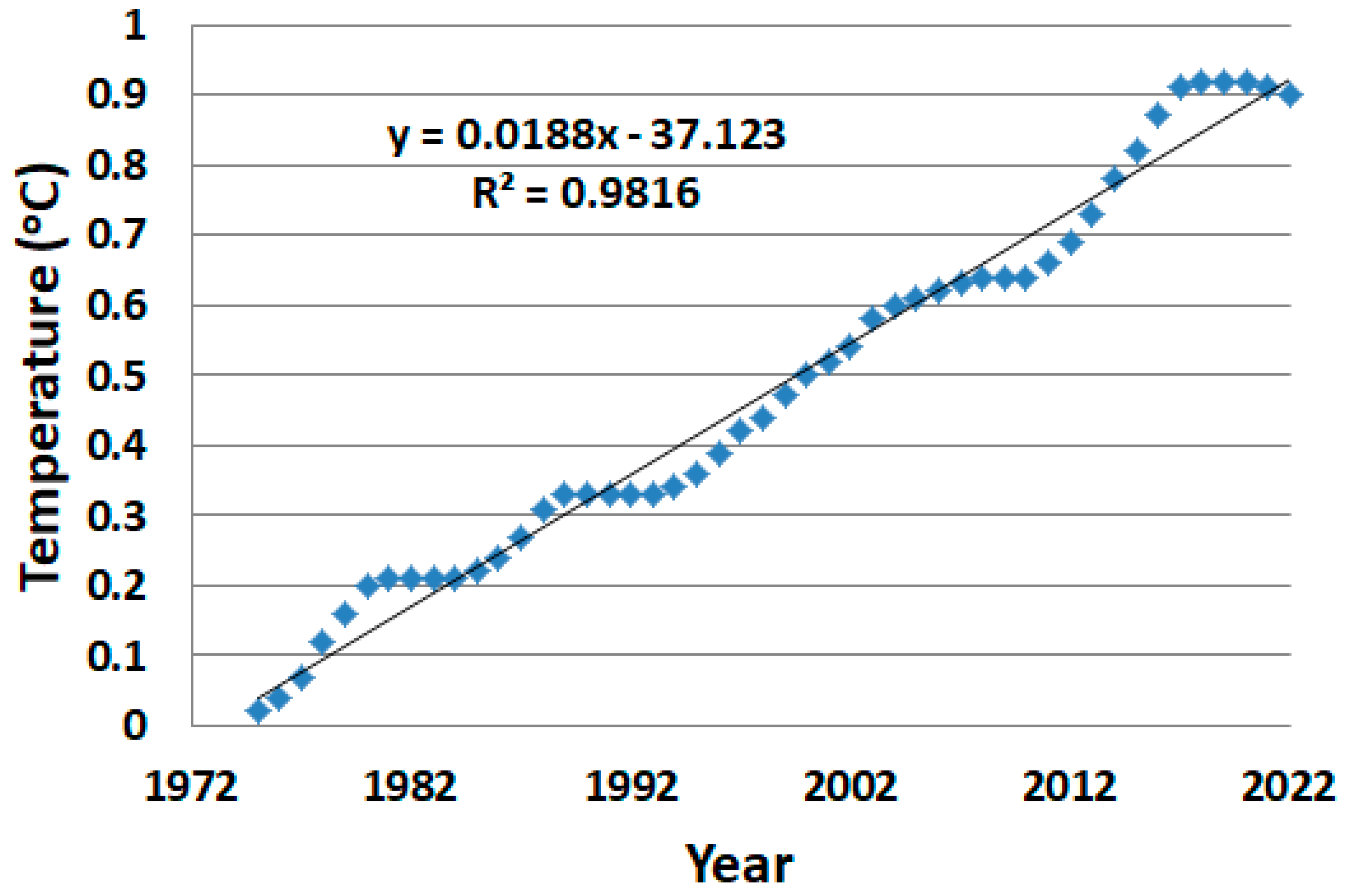
2.2. ASG Temperature Reversal Estimate

In this paper, the approach is to provide key physics-based equations and SRM area estimates to achieve just enough solar geoengineering to reverse the potential yearly increase in global temperatures, which we can refer to as annual solar geoengineering. For example, global warming from 1975 to 2022 was 0.9 °C [26]. If a status quo annual solar geoengineering approach was applied, the ideal result would be a zero temperature increase, stabilizing global temperatures. The warming level would stay at 0.9 °C. According to Figure 1, the temperature reversal (TR) up to 2022 requirement for ZGWG per year is (see also Appendix E)
TR = −0.0188 °C/year
Figure 2 breaks down the warming for land and ocean, whereas Figure 1 is due to a mixed temperature results. Here, we note that warming over land is hotter than over the ocean, with slopes of 0.0327 °C/year for land and 0.012 °C/year for ocean warming. Figure 1’s slope is close to the weighted average, with 30% of the GW over land and 70% over the oceans, yielding the weighted average slope in Figure 1 of 0.0188 °C/year (≈0.0327 °C/year × 0.3 + 0.12 °C/year × 0.7). In this paper, ASG estimates are based on the mixed average slope in Figure 1, similar to the estimates from other authors [12]. However, the ASG equation goals can easily be adjusted depending on the reader’s interests.
Note that the recent trend with the large increase in global temperature in 2023 suggests that the warming has increased enough where the slope in Figure 1 appears to have changed to around 0.027 °C/year since the initial work in this paper (a 45% increase). This is in part related to the strong El Niño effect in 2023 and is discussed in more detail in Appendix E. Please note that the next La Niña may reduce this 2023 trend as a slope of about 0.02 °C/year has been a standard value up until recently. The reader may wish to update the goal in Equation (6) and/or in the supplementary SG calculator, which is the affected key-related value to account for this anticipated new global temperature increase per year.

2.3. Theory

In this section, key physics-based ASG equations and goals are presented. The numbers used in this section and Section 3 can be updated for more complex computer-aided models depending on the reader’s interest and the changing climate. A list of symbols used in this paper with definitions is presented in Table 2.
In the results in Section 3, averages for approximating estimates are mostly used. The estimated general requirement to offset a temperature increase in energy units from the slope in Figure 1 is
TR = −0.0188 °C/year = −0.102 Wm−2/year
This conversion to energy units is obtained (using the Stephan–Boltzmann relation) as
Δ P Re v = P 2 P 1 = σ ( T 2 4 T 1 4 ) = 0.102   Wm 2
where T1 is taken as the average surface temperature of the Earth of about 14.5 °C and T2 = 14.5 °C + 0.0188 °C = 14.519 °C. Note that Equation (3) is simply a direct conversion from the observed temperature increase per year to energy units. This value contains both feedback and forcing, as indicated in Equations (4)–(6) (see also the SG calculator in Supplementary Materials).
The SG strategy indicates that reversing global warming that occurred from 1950 to 2019 having a temperature rise of 0.95 °C, would require a reversal of Δ P Re v = 5.15   Wm 2 . This is just the global warming rise from 1950 to 2019 of 0.95 °C in energy units, where Δ P Re v = σ ( T 2021 4 T 1950 4 ) = 5.15   Wm 2 = σ ( 288.6 K ) 4 ( 287.65 K ) 4 . Here, 287.65 K = 14.5 °C is roughly the average temperature of the Earth around 1950. The 5.15 Wm−2 consists of forcing and feedback. Feedback typically doubles the forcing. We use a feedback amplification factor of 2.15 {28, 30], as discussed below. Therefore, about 2.4 Wm−2 is due to forcing (i.e., 2.15 × 2.4 Wm−2 = 5.15 Wm−2). Then, we can write for full global warming mitigation with the background climate parameters considered (from 1950 to 2019), the reversal equates to [25]
Δ P Re v = 5.1   Wm 2 = Δ P T ( 1 + f ) A ¯ F
In this equation, we require a GW reversal of Δ P Re v = 5.15   Wm 2 , which in theory can be accomplished with a large albedo SRM surface area change to what is termed here as the target area. Then, in Equation (4), we note that:
  • The reverse forcing of the target SRM area required is denoted by Δ P T . We note that three things happen in SRM: (1) we increase the albedo reflectivity of a hotspot surface target, causing a reverse forcing of Δ P T ; (2) this also reduces its associated greenhouse gas re-radiation background climate effect since there are fewer long wavelengths emitted from the SRM area, which means a reduction in re-radiation; and (3) there is also a reduction in water vapor GHG feedback due to the cooling of the hotspot target. Other feedback may also show some reversal.
  • The GHG re-radiation reduction is estimated in Equation (4) using the 1 + f term. Here, f is the re-radiation estimate average of about 62% [28,29]. This is the average re-radiation that occurs in our atmosphere in 2023.
  • In this equation, we assume that feedback, which is dominated by water vapor, will also reverse as part of the background climate cooling effect. That is, SG reverse forcing causes a cooling effect and cooler air holds less water vapor. In Equation (4), the average feedback amplification factor, including water vapor feedback, is estimated in 2019 as A ¯ F = 2.15 [28,30]—see also Appendix D for the conversion to feedback units. We note that many other authors have anticipated that water vapor feedback likely has a doubling effect [31,32], so a factor of 2.15 is reasonable. Note that this value can be written with temperature dependence, and this is discussed in Appendix A.
Then, inserting A ¯ F = 2.15 into Equation (4), we find the estimated SG target reversal goal for a global warming reduction of 0.95 °C is
Δ P T = 5.15   Wm 2 A F ( 1 + f ) = 2.4   Wm 2 ( 1 + f ) = 1.48   Wm 2
This is the estimated recommended target reverse forcing goal needed for a total reversal of global warming from 1950 to 2021 of 5.15 Wm−2. To achieve this, we only require an equivalent solar radiance reduction of 0.44% (=1.48 Wm−2/340 Wm−2). Taking into consideration the background climate helps minimize estimates. This is compared with other authors [4,5,6,7,8,9], who have used higher estimates. Other updated estimates may be used depending on the reader’s interest. Since, in this paper, we are interested in stabilizing global warming annually, the ASG albedo SRM target goal requirement for a yearly reversal is approximated similarly to Equation (5) as (from Equations (3) and (4))
Δ P A S G = Δ P T = Δ P Re v ( 1 + f ) A ¯ F = 0.102   Wm 2 / Yr ( 1.62 ) ( 2.15 ) = 0.0293   Wm 2 / Yr
This is the estimated main reverse forcing ASG target goal recommendation used in this paper with background climate effects included (see Appendix E for recent trends that suggest this goal may be 45% too low according to new 2023 data). Note that the ratio of Equation (5) to Equation (6) yields a reverse forcing reduction by a factor of 50. The results in Equation (6) are based on the slope of GW data observed from 1975 to 2022 in Figure 1 and Equations (2) and (3). As long as this slope remains constant over time, as in Figure 1, the yearly goal in Equation (6) will likely be adequate each year. However, if the slope changes due to excessive GW increases, then we need to update Equations (2) and (3), which will change our Equation (6) goal (the reader may wish to use the supplemental solar geoengineering calculator provided with this paper).

2.3.1. SG Advantage and the Greenhouse Gas Equivalent Reduction from SRM

It is helpful to note the SG advantage in Equation (5) as motivation, since there is often pushback to using SG, which is an important underfunded tool to help mitigate climate change. Furthermore, this will also illustrate the strong effects that negative solar geoengineering has (as discussed in Section 4.1.6).
To mitigate the 5.1 Wm−2 in Equation (4) requires an estimated SG change of −1.48 Wm−2, as shown in Equation (5), compared to trying to achieve this with GHG removal, which would require the full −2.4 Wm−2 (Equation (5)). This yields a work saving of 0.92 Wm−2 (=2.4 Wm−2 − 1.48 Wm−2). This is a 38% (=0.92 Wm−2 /2.4 Wm−2) advantage for SG [28], yielding much less effort and higher work efficiency compared to CDR. In CDR, two things happen when GHG is removed, whereas in SG, three things happen. This creates the 38% higher efficiency compared to CDR. In CDR, we have (1) a reduction in the GHG effect, and (2) this causes a feedback reduction. In SRM, for example, (1) we cool an area with SRM, (2) this causes an additional reduction in the GHG effect as there are fewer emitted LWs that can be re-radiated, and (3) this causes a reduction in water vapor feedback from the cooling. That is, in SG, fundamentally, we include a 1 + f re-radiation reduction GHG background climate effect in Equation (5) (i.e., increasing the reflectivity of a hotspot surface also reduces its associated greenhouse gas effect).
This is a key effective advantage of SG that this paper recommends when working on SG mitigation goals. Therefore, 38% of SRM includes an additional ‘GHG-albedo equivalent reduction’.
This GHG-albedo SG effect may also, in certain areas, decrease the high levels of possible CO2 and often water vapor feedback re-radiation that can occur in UHIs in the presence of high heat flux using SG [2,33].
Furthermore, both SRM and CDR cause a cooling effect, reducing water vapor in the atmosphere and its associated feedback. So, SRM reduces the GHG effect as well.
Alternatively, worldwide negative solar geoengineering equivalently increases the GHG effect by this 1 + f factor (Section 4.1.6), and its additional associated water vapor feedback increases from the background climate effects. When these average effects are considered in addition to the background climate and UHI microclimate amplification (HT), urbanization heat fluxes from impermeable surfaces can be problematic on both the local and global levels [2,3,33], as discussed in Section 4.1.6.

2.3.2. SRM Area Estimates for Annual Solar Geoengineering

To estimate Equation (6)’s area modification requirements for a −0.0293 Wm−2 reversal, the approach involves using the following updated solar geoengineering equation based on Feinberg [25], given by
Δ P T = Δ P A S G = S o 4 A T A E X C X O X S H T ( Δ α T )
The key updates in this equation compared with the author’s prior work are as follows: in my prior study, the Δ P T goal was for a full GW mitigation, which equated to Equation (4). However, in ASG, the goal is reduced by a factor of 50 so that Δ P T = Δ P A S G = 0.0293   Wm 2 / Yr . In addition, the factors X O and X S are added and are described below.
To aid the reader, an overview of Equation (7) is as follows:
  • This SG physics-based equation indicates that in SRM, as anticipated, the reversal is proportional to the average solar energy over 24 h and is given by S o / 4 .
  • The fractional albedo SRM target area change required is denoted as AT. This change is taken relative to the Earth’s area AE.
  • The amount of irradiance Xc falling on the target has a global average of X ¯ C = 47 % [29] of sunlight passing through the clouds. This can vary depending on the location. This value can be changed in the model depending on the target’s location.
  • The amount of outgoing reflected transmission from the target is denoted by X O . This is primarily used in albedo Earth brightening applications (see Section 3.1). This is just the amount of reflected sunlight from Earth brightening that is anticipated to make it into outer space due to potential issues such as clouds and aerosol particulates. A Bayesian probability estimate for this value is provided in Section 3.1.
  • The space irradiance factor denoted by X S (see Section 3.2) is typically 1 for non L1 space mirror applications. However, for L1 space mirror applications, the optimal L1 point rotates around the Sun with the same angular speed as the Earth, thus allowing constant sunshading. Then, the sunshading irradiance occurs 24 h a day and the Earth’s curvature is not a factor. This increases So/4 to So. To account for the increase in space irradiance, we can let XS = 4 in Equation (7) for L1 space mirror applications.
  • The albedo change of the target is denoted as Δ α T = α T α T , where the target’s albedo originally has a value of α T , and when we apply an SRM, its albedo increases to a new value denoted by α T .
  • Lastly, included is an UHI de-amplification factor H T . This is for targets in urban heat island (UHI) areas which can have UHI microclimate de-amplification effects, denoted by HT [2,33,34]. For example, in UHIs, the solar canyon effect amplifies warming when buildings reflect light onto pavements, increasing the irradiance and amplifying the temperature at the surface. Other amplification issues can include re-radiation due to the increase in local CO2 GHGs, local water vapor feedback, temperature inversions, loss of wind and evapotranspiration cooling, increases in the solar heating of impermeable surfaces from building sides, pavements heat fluxes, and so forth [2]. Some of these microclimate amplification effects could reverse and de-amplify in ASG urban applications, increasing cooling, and can be accounted for in Equation (7) with the HT variable. City heat flux amplification is often observed by the UHI’s dome and footprint. The footprint and dome growth are indications of amplified heat flux that is observed to spread beyond the boundaries of the city itself, both horizontally and vertically [2,34,35]. Using ASG, the footprint, dome effects, and city temperatures can be reduced.

3. Results

3.1. Earth Brightening Transmission Loss

In Equation (7), the XO factor provides an estimate of the outgoing transmission of reflected short-wave sunlight radiation and is applicable in Earth brightening albedo methods. When taken as unity, the results for Equation (7) in Earth brightening applications yield the minimum required albedo SRM area to achieve a specific ASG reversal goal. In Earth brightening, several eventual losses can occur for the outward reflected short-wavelength transmission through the upper atmosphere. The primary losses are clouds and aerosols that can impede the reflected sunlight [36]. These losses in the upper atmosphere areas can affect the mean lower surface air temperature (MSAT).
The incoming solar irradiance XC in this paper is taken as 47% due to clouds, as indicated in the IPCC global mean Earth energy budget assessment [29]. However, one might anticipate that the outgoing radiation transmission from an Earth-brightened SRM surface area will have a higher transmissibility probability than the incoming irradiance. For example, given that the incoming sunlight radiation occurred through a clear portion of the sky, we can estimate the probability that there will be loss issues on the outgoing reflective radiation, which should be less. One helpful estimation method is to use a Bayesian approach. Using this prior information that the sunlight makes it to the target, the Bayesian result indicates that the probability of clear transmission is 78%. This is estimated in Appendix B. Therefore, the minimum required albedo SRM area obtained in Equation (7) for Earth brightening is adjusted in this paper using a Bayesian correction by the XO-Bayes’ = 0.78 factor.
Readers may wish to model this further for specific areas and adjust this factor using other probability methods and factors (such as aerosols) to improve transmission estimates. One should note that it may not be well known how transmission loss affects the MSAT. In addition, there are areas for Earth brightening where SRM is optimal, such as near the equator, yielding higher irradiance and where XO-Bayes’ may be close to a value of 1 [36].

3.1.1. Pavement and Roofs

As an example, consider the required area for worldwide cool pavements and/or roofs. We can consider an average asphalt pavement/roof albedo of about α T = 0.1 , and using cool roads and roofs, the estimated increase for a target pavement/roof area in this example is taken as α T = 0.4 . Then, considering an average irradiance of X C = 0.47 , with X S = 1 , H T = 1 , and A ¯ F = 2.15 , and using the reversal goal (Equation (6)), the requirement is
Δ P A S G = S o 4 A T A E X C X O B a y e s X O M i n i m u m X S H T ( α T α T ) = 340   Wm 2 A T A E 0.47 0.78 1 0.3 = 0.0293   Wm 2 / Yr
Solving this, we obtain the SG target area percentage for ZGWG, yielding a minimum and Bayesian estimated requirement of
A T A E = 0.078 % per year B a y e s 0.0611 % per year M i n i m u m
The pavement and/or roof albedo SRM area that needs to be cooled for a Δ α T = 0.3 change equates to
A T = 0.000778 per year B a y e s 0.000612 per year M i n i m u m × 196.6 E 6 mi 2 = 154,048 mi 2 per year B a y e s 120,158 mi 2 per year M i n i m u m
This yields an equivalent minimum radius of 196 miles. This result is summarized in Section 3.4. This example illustrates the albedo SRM area modification requirements for ASG. Other values may be used depending on the reader’s interest.
For hotspots pavements and/or roofs in humid areas that are cooled with the feedback factor dominated by water vapor and A F = 4.3 (see Equation (A4)), the requirement for area modification is much less according to Appendix A. In this case, we also increase Δ α T > 0.3 to Δ α T = 0.5 for this example. The area modification is reduced from Equation (10) to
A T = 46,182 mi 2 per year B a y e s 36,022 mi 2 per year M i n i m u m
This yields a reduced equivalent minimum radius of 76 miles. This result is also summarized in Section 3.4. Note that to achieve these results, the goal is reduced by more than half.
If we could achieve full global warming SG mitigation for the equivalent cool pavements and/or roofs in Equation (10), but with Δ P = 1.47   Wm 2 , Δ α T = 0.3 , and A F = 2.15 , the area required would be about 6 million square miles. In comparison, for this ASG requirement, where Δ P A S G = 0.0293   Wm 2 / Yr , Δ α T = 0.5 , and a hotspot mitigation estimate for A F = 4.3 (see Equation (A4)), the resulting area is reduced to 36,000 mi2 and is a factor of 160 smaller.
Yearly mitigation estimates can vary and will depend on Δ α T and the amount of feedback reduction each year, which can be difficult to estimate. However, similar mitigation is needed each year until CDR and CO2 reductions become significant. This is illustrated for different RCP scenarios in Section 3.5, as ASG projections are also dependent on RCP estimates.

3.2. L1 Space Sunshade Estimates

We can find an AT area modification requirement for a solar reflective space disc mirror-type sunshade application. In this case, we note that most authors consider the Sun–Earth L1 position as optimal. For the irradiance in space mirror sunshade estimation, we can take XC as 100% and XS as 4 (as discussed above). Sunshading can effectively translate to changing the reflectivity of a target on Earth’s to ~100% from the average Earth’s albedo of 30%, so that Δ α T = 0.7. Using these parameters and our ASG goal, Equation (6) is
Δ P A S G S p a c e M i r r o r = X S S o 4 A T A E X C ( α T α T ) = 1361 Wm 2 A T A E ( 1 ) ( 0.7 ) = 0.0293 Wm 2 / Yr
Solving this, we obtain the ASG percentage for ZGWG of
A T A E = 0.003 % per year
This yields a disc of about 15,686 km2 (radius 71 km). Section 3.4 summarizes this result. Sánchez et al. (2015) indicated an area-to-mass ratio near 4 × 10³ kg/km2. Using this, the weight required for an area of 15,686 km2 would roughly be about 63,000 tonnes. We might consider a reflective particle option. However, the injection requirement for SO2 reflective particles assessed in Table 3 is 313,000 tonnes. This is surprisingly higher. However, Appendix C finds lower values of 21,000 tonnes for CaCO3 and 41,000 tonnes for SO2 that may be more applicable for L1 space sunshade applications. Nevertheless, given that these are yearly requirements; this further indicates yearly challenging issues.
When we talk about space mirrors with a value for AT/AE, this value also yields the required percentage of incident solar radiation that is needed to be reflected away from the Earth to achieve a mitigation goal in Equation (12). Note that Equation (13)’s value is reduced by a factor of 556 (=1.7%/0.003%) compared to the requirements for full mitigation, as estimated by other authors for a reduction in solar insolation of 1.7% to offset the effects of a doubling of CO2 concentration [5,6,7,8]. However, it is only reduced by a factor of 51 compared to the author’s initial paper [25], with a goal of 0.154% reduction required to reverse a 1 °C rise in 2021. Lastly, note that the yearly required increases are estimated in Section 3.5 for different RCP scenarios.

3.3. Annual Stratospheric Injection Estimates

The results demonstrate that it is quite challenging to meet the ASG area modification requirements (summarized in Section 3.4) for both Earth brightening and space mirror size estimates. Unfortunately, there is no easy solution. Although this paper does not focus on SAI, as it is often assessed with computer climate models, it is helpful to overview the ASG goals and estimated differences compared to full GW mitigation. In this section, basic ASG injection rates are estimated.
Much has been written about an alternate less expensive Sun-dimming temporarily reflecting particle method such as SO2 injected into the stratosphere [37,38,39,40,41,42]. Here, SO2 injected into the stratosphere at the top of the atmosphere (TOA) reduces the Sun’s energy reaching the Earth through solar aerosol reflectivity. As an estimate for annual SAI, we can use the equation given by Niemeier and Timmreck [13], where the reduction in radiation at the top of the atmosphere Δ R T O A is
Δ R T O A = 65   Wm 2 exp ( 2246 Mt [ SO 2 ] Yr 1 / I S O 2 ) 0.23
The actual injection rate I S O 2 (in units of Mt[SO2]/year—megatonnes of SO2 per year) for full GW reduction according to Equation (6) requires a goal of 1.47 Wm−2. To provide the first-year annual requirements rather than full mitigation, the injection rate using Equation (14) is 22-fold lower, as shown in Table 3. Here, full climate mitigation requires an injection of 6.9 Mt[SO2]Yr−1 for a goal of 1.47 Wm−2, whereas for the first year, the ASG goal is reduced to an injection of 0.313 Mt[SO2]Yr−1 for a Δ R T O A = 0.0293 Wm−2 goal (Equation (6)). Unfortunately, depending on the SO2 dissipation per year, this would possibly need to be doubled in the second year, tripled in the third year, and so forth to stabilize global warming annually. We note that Izrael et al. [12] estimated an injection rate of 0.25 Mt[SO2]Yr−1 as the cumulative requirement for global temperature stabilization at +2 °C starting in the year 2050. This injection rate is close to the estimate provided here of 0.313 Mt[SO2]Yr−1 for a 0.0293 Wm−2 goal. Jones et al. [14] noted that “In GEO4.5, the injection rate increases monotonically to attain a peak value of 10.9 Mt[SO2]Yr−1 in 2080 following which it plateaus as global warming in RCP4.5 stabilizes at slightly above 3 K”. This is over 60 years and is close to the full reversal estimate in Table 3 of 6.85 Mt[SO2]Yr−1.
The cumulative yearly required minimal increases are estimated in Section 3.5 for different RCP scenarios. In Appendix C, a helpful area coverage estimate is provided and uses the alternate method of Section 2.3.2 (discussed in Appendix C) and illustrates ideas on SAI testing. The stratosphere area modification required has not been fully established, as assessments are usually provided on injection rates that are often equated to one Pinatubo eruption, which may need to be refined. The initial maintenance assessments in Appendix C will depend somewhat on the reflection efficiency, which may require testing.

3.4. Overview of Estimates

Table 4 provides an overview of the needed estimates based on the suggested inputs to mitigate the annual global warming growth trend of 0.019 °C/year for ASG. Also available in the Supplementary Materials is a solar geoengineering calculator for Table 4, which may be helpful for the reader. The results in Table 4 provide mixed options, with Earth brightening area modifications of surface land and space-type applications. The objective for each is to reduce the incoming solar energy by 0.0293   Wm 2 / Yr . This goal can be divided up by reducing the albedo SRM area requirements proportionately. Therefore, one could divide up the results for numerous combinations (see also Section 4.1.5) to meet the ASG requirements. Note that in Table 4, the HT value, as an example, is taken as 3 for UHI areas and conservatively as 2 for Earth mirrors used on urban rooftops, as often implemented by Project MEER [24]. This HT average estimate can vary depending on the UHI microclimate [2]. In the case of something like sea-type floating mirrors or reflective particles [43], HT = 1, as shown in Table 4.
Note that the ASG requirements (Equation (6)) compared to full mitigation (Equation (5)) are reduced by 50 times (=1.47 Wm−2/0.029 Wm−2) in energy flux requirements and albedo SRM area (per Equation (7)). For example, desert treatment is reduced from the author’s initial estimate of 1.0% [25] to 0.02% for annual mitigation in Table 4. Therefore, the areas in ASG mitigation are, in general, 50 times smaller, which also minimizes any potential circulation concerns [17,18,19,20,21]. Table 4 suggests several options including multiple combinations that can be considered in annual mitigation, as suggested in Section 4.1.5. In this section, the SRM methods are also rated. For hotspot cooling shown in Table 5, this has the potential to reduce area requirements by a factor of over 150 (per Equation (11)) due to a combination of Δ α and larger feedback changes in high-humidity areas. The yearly required minimal increases are estimated in the next section for different RCP scenarios.

3.5. RCP ASG Cumulative Area Estimates

The ASG requirements detailed in this paper assume increases from about 2023 to when manmade GHGs substantially decline. Table 6 provides some ASG cumulative estimates anticipated with two different RCP scenarios. The ASG estimates are based on the results in Table 4 times the number of additional years required for the RCP scenario peak [44] plus a rough estimate of the number of years needed for GW thermal equilibrium to occur. An estimate of a 10-year allowance period after the peak amount of CO2 is reached for the thermal equilibrium time period is established, as shown in Table 6. This rough estimate is based on the results of global circulation models that indicate that about 85% of the GHG GW effect occurs in the first 5 to 10 years [2,45]. Near the peak, the CO2 and the GW increases should start to taper-off. This additional reduction should aid in reaching thermal equilibrium in the 10-year allowance period. Further, ASG estimates can be refined as needed.

4. Discussion

4.1. Annual Solar Radiation Management

4.1.1. Annual Solar Geoengineering Allocation by Country

To aid solar radiation management, we can allocate goals amongst countries by their wealth. For example, using the total household wealth by county, the United States and the United Kingdom’s requirements would be 31% and 3.5% [45,46], respectively. Then, the minimum area allocations, for example, with surface albedo change Δ α T = 0.3 in Equation (10) would be:
  • The US’s mitigation = 31% × 120,158 mi2 = 37,249 mi2/Yr or 102 mi2/day
  • The UK’s mitigation = 3.5% × 120,158 mi2 = 4205 mi2/Yr or 11.5 mi2/day
Such goals may be obtainable with many of the different SG technology methods (see Section 3.4 and Section 4.1.3).
The costs associated with solar geoengineering in space sunshading can similarly be divided.

4.1.2. Implementation Using L1 Space Particle Clusters

Another similar idea that may merit investigation is to use space particle clusters instead of space mirrors, at or near the L1 Sun–Earth region. This idea has been suggested in the past [47]. A cluster of particles such as calcium carbonate, SO2, or moondust [9] in space at L1 may have a long suspension time, reducing the injection rate. Diffusion would likely be slow due to low outer space temperatures (~2.7 K), and studies could be performed to estimate issues.
We can estimate the requirement for solar reduction for an ASG value using a transmissibility method [25]. For example, considering that the Earth’s solar absorbed radiation estimate is S o 4 ( 1 0.3 ) = 238.175   Wm 2 , a required absorption reduction estimate can be found for Equation (6) from
S o 4 ( 1 0.3 ) = 238.175   Wm 2 0.0293   Wm 2 = 238.1457   Wm 2
Solving this yields So = 1360.833 Wm−2. Then, one finds that 0.167 Wm−2 (=1361 Wm−2 − 1360.833 Wm−2) is the reduction required for the incoming solar radiation.
If we measure the transmission of the incoming solar radiation above and below the particle treatment, the transmissibility (TR) from sun-dimming should be [25]
T R = 1360.833   Wm 2 / 1361   Wm 2 = 99.9877 %
Measuring the transmissibility is likely a helpful method to assess the injection amount. Note that we can also use similar measurement methods for SAI.

4.1.3. Earth Brightening Advances

Earth brightening SG’s state-of-the-art potential is a lot higher today. Drone technology, for example, has led to major advances in painting buildings [48] and agriculture spray methods [49]. For example, consider the US and the UK’s goals for Earth brightening in Section 4.1.1 in terms of area per day:
  • The US’s mitigation goal for Earth brightening is 102 mi2/day
  • The UK’s mitigation goal for Earth brightening is 11.5 mi2/day
A typical two gallon per acre agriculture drone can spray about 1 mi2/day [50], which includes refills. Then, if we assume that paint drones can be designed with similar capabilities, this may require feasible areas as follows:
  • For the US’s mitigation goal, about 102 drones/day
  • For the UK’s mitigation goal, about 12 drones/day
However, paint areas have to be made available. This can include urban rooftops and cooling roads. ASG applications in UHI and other areas are a large undertaking and as we can see, the amount of brightening applied per day, even with drones, will require AI technology. This is also true if applied to UHI areas. Therefore, it is vital for technological agencies like NASA, Space X, and the Canadian, Chinese, and European space agencies, etc., to become involved to accomplish this on the large scale needed. This AI technology should be part of the solution but will not occur without this type of effort.
Although paint drones are not equivalent or rated similar to agricultural drones, technology improvements will likely be able to provide this type of capability for paint drones. Given the technological advances in AI, improvements in Earth-brightening drones, while difficult, are likely more feasible than one might think. The helpful solution will likely require a mixture of ASG Earth brightening technologies (Section 3.4 and Section 4.1.5).
New ultra-thin bright white paint surface treatments (98.1% reflective and half as thick) have been developed to help cool the Earth [51,52]. Other technologies could possibly be developed specifically for the Earth brightening of buildings, streets, desert areas, mountain tops, and UHI areas. Again, this requires agencies like NASA, Space X, and the Canadian, Chinese, and European space agencies, etc., to vastly improve AI drone use for SG implementation. AI technology could allow for 24 h-a-day drone ASG work with automatic target brightening, refilling, and target recognition. Furthermore, studies could help to assess the best strategies to try and improve coverage areas including mountain ranges, since mountains cover about 24% of the Earth. Brightening mountain areas could also increase condensation and snowfall, as was achieved on the Peruvian Andes mountain tops [53], which can increase snowfall and spring runoff to reservoirs in drought-prone areas.
Annual mitigation using Earth-based mirrors, as suggested by Project MEER [24], has several advantages. Mirrors can be placed in areas of high irradiance, likely yielding a large albedo change, and when used in city areas on roofs, we can estimate that HT > 1. These reduce the Earth’s annual SG area requirements, as per Equation (7). Alternatively, it may be of interest to use something like sea mirrors or reflective floating particles which would yield a high albedo change, as exemplified in Table 4.
One might question the practice of painting the Earth a light color. Yet, we continue to accept negative solar geoengineering (Section 4.1.6) essentially painting the Earth with dark colors on roads, roofs, and building sides. Unfortunately, we are already at the point where we are faced with these types of difficult decisions [23].

4.1.4. Natural Hotspots

Natural hotspots like deserts and mountain areas are likely good ASG targets to consider in order to find ways to cool them to help to reduce global warming. Here, hotspot cooling produces a high albedo change similar to pavements and asphalt roofs, reducing area requirements as per Equation (7). In humid areas, larger feedback reductions can also be obtained. They also may cover a significant area and are relatively free from urbanized regions. Similar to pavements and UHIs, natural hotspot cooling would likely help to reduce atmospheric water vapor feedback (see Appendix A). Also, certain regions are optimal, such as the tropics and subtropics [36], for humidity feedback reduction. Certainly, natural hotspots would be highly controversial geoengineering targets. Nevertheless, their amplification of heat and its effect on the Earth’s temperature will likely be related to their area and temperature differences compared to the global ambient temperature. Some examples of such hotspots that we could find ways to cool include:
  • Flaming Mountains, China
  • Bangkok in Thailand (the planet’s hottest city)
  • Death Valley, California
  • Deserts
  • The badlands of Australia
  • The tropics and subtropics

4.1.5. ASG Methods Rated with Mixed Planning

A mixed SG plan similar to Table 4 for annual global warming mitigation of −0.019 °C/year can reduce the burden of relying on any one method, which would reduce governance issues and unforeseen problems regarding technological SRM. A mixed ASG plan should include ocean reflective particles or floating mirrors, AI drone painting, space mirrors or clusters as well as the traditional ideas of stratospheric aerosol injection, marine cloud brightening, and cirrus cloud thinning. Each method will typically have issues and consequences. These consequences may require future planning. For example, cool roads can hamper snow melting in winter regions and SAI can create area farming problems. One may anticipate that cloud brightening and cirrus cloud thinning are not high-level solutions due to the large required areas found in Table 4 and Table 6. In mixed planning, it is helpful to have ratings for ASG SRM methods. Table 7 provides an overview of the author’s ratings for each ASG method, which may be helpful.
In addition to ASG, the author has estimated that half of the annual warming increase is due to population growth [30]. That is, under zero population growth, we would anticipate a slope reduction to about 0.01 °C/year in Figure 1. Non-SG efforts in the area of population development supported by multi-country governance would be extremely helpful according to this recent study [30]. The importance of annual global warming mitigation is key to the success of strategies to address the immediate yearly GW trend occurring, as we are close to crisis levels. This should also include a strong effort to reduce negative solar geoengineering as well.

4.1.6. Worldwide Negative Solar Geoengineering

Stabilizing global warming annually is challenging enough. However, the problem of yearly increases in the number of black asphalt roads, rooftops, and even dark-colored cars worldwide makes the task harder. Although many issues, such as black electric vehicles and gas cars, do not contribute significantly to global warming, they encourage bad practices of poor solar color choices. This illustrates the lack of SG awareness, which is highly problematic for an increasing population [33]. As a suggestion, restricting cars to light colors would go a long way in greatly increasing such awareness.
In terms of global warming, these issues are a form of negative solar geoengineering and contribute significantly to the urbanization GW problem. Feinberg [2] and Zhang et al. [3] have estimated an approximate 13% urbanization GW effect due to the solar heating of impermeable surfaces and about half due to anthropogenic heat release [2]. In UHIs, heat fluxes are often also amplified by the microclimate (HT). Currently, it is estimated that roads occupy about 14% of all manmade impermeable surface areas [54] of which impermeable surfaces occupy an estimated 0.26% of the Earth’s surface [55]. Then the estimated area of the Earth occupied by roads is small, at about 0.0364%. This is on a similar scale compared to Equation (9) estimated requirement for area modification and illustrates the negative ASG interference issue. Compared to the estimated total area of impermeable surfaces, it is a factor of 8.5 times higher than the Equation (9) requirement (0.26%/0.0305%). This illustrates the difficult task of annual surface area modification requirements with the worldwide negative SG interference. Feinberg [2] estimated that 1.1% of global warming is likely due to asphalt roads using only an average background climate feedback factor, which, if brightened similar to concrete, with an albedo increase factor of 5, could have reduced global warming by 5.5%. In humid areas this improvement can be 2-fold higher (Appendix A). An MIT pavement study [56] concluded that in all US urban areas, an increased temperature of 1.3 °C occurs in summer months and heatwaves are 41% more intense with 50% more heatwave days due to asphalt pavements. The expansion of cities is increasing rapidly where 55% of the world’s population lives and this is expected to grow to about 70% by 2050 [57].
Feinberg [25] estimated that heat from asphalt roads and roofs can produce 7.5 times more energy in heat pollution per acre (2.5 GWh) than a solar power plant, where studies have found solar plants average about 0.33 GWh per acre per year [58]. Furthermore, a gallon of gas equates to 33.6 kWh [57]. Then, this heat pollution equates to 74,200 gallons of gasoline energy per year per acre.
This illustrates the enormous amount of energy in the form of heat pollution produced by an acre of asphalt, and indicates how black roads and roofs make significant incremental contributions to warming locally. In wooded areas, this heat pollution can contribute to drying out forests and contribute to forest fire concerns.
Negative SG also has the potential to increase local and global water vapor feedback as it creates increases in warm air, which can hold more water vapor. Hotspots per unit area can increase water vapor feedback dramatically, as illustrated in the assessment in Appendix A and Section 3.1.1. Zhao et al. [59] observed that UHI temperatures increase in the daytime (ΔT) by 3.3 K more in humid climates compared to dry climates. A primary issue in humid UHI areas is the use of black asphalt, which, given the worldwide problems from urban heatwave, this author feels should be banned in most cases. The warming consequences of black asphalt are not fully understood, but it is bad for the local environment and is well documented as being linked to many problems, especially in concentrated urban areas where heatwaves cause related health issues [56,60]. A Smart Surfaces Coalition [61] using cool roads, roofs, and other methods has shown success in the US city of Baltimore, lowering heat by 5 °F and reducing the cooling cost approximately 10-fold. Ten new cities, including Atlanta, Boston, Dallas, New Orleans, Columbia, and Phoenix, are currently adopting similar methods, but more effort needs to be made worldwide to stop negative SG. Such issues should be addressed in global climate meetings. For example, albedo goals are urgently needed and should be added to the Paris Agreement as SRM is the best tool to offset negative SG.

5. Conclusions

In this paper, estimates are provided for annual solar geoengineering requirements. The results illustrate many challenges. However, the results show higher feasibility for annual solar geoengineering modification to help to mitigate global warming. This is due to reductions in goals that lead to a factor of 50 to possibly over 150 times less albedo SRM area requirements compared to full SG mitigation. This minimizes circulation concerns and many other controversial issues.
Many recommendations are provided in this paper. These include the recommendation to use ASG, its goal (Equation (6)), the associated geoengineering equations (Equations (4), (7), (8) and (12)), the use of mixed technology (Section 3.4 and Section 4.1.5) for Earth brightening modification, related ASG SRM estimates (Table 3 and Table 4), the suggested method of using L1 space clusters that may be highly useful (Section 4.1.2), and the use of the HT microclimate amplification value in UHIs, as shown in Table 4. The results in general point to challenging but feasible solutions. It is vital for agencies like NASA, Space X, and the Canadian, Chinese, and European space agencies, etc., to help to develop the technologies required for ASG implementation. Much work is needed, especially in the area of L1 space sunshading (see Section 3.2 and Section 4.1.2) and to assist in the development of AI drone paint tools for Earth brightening (see Section 4.1.3 discussion).
Suggestions are provided for solar radiation management using wealth allocations by country for ASG to improve feasibility (Section 4.1.1).
It is pointed out that for ASG to be effective, it is helpful to address many global warming issues, including the ongoing negative solar geoengineering, especially the practice of black asphalt use (Section 4.1.6). We should not condone the bad practices of dark color choices, whether it be in the automotive industry or the construction practices of roads, houses, and buildings. This also impedes positive ASG efforts. Such issues are currently unaddressed in worldwide climate meetings.
It is likely important to have a mixed plan (Section 4.1.5 and Table 7) that includes annual global warming mitigation strategies that could include, in addition to ASG, the likely need for population (limited or no growth) development supported by multi-country governance to reduce warming due to anthropogenic effects (Section 4.1.6).
There is little time left to meet the IPCC’s suggested 1.5 °C goal. The longer we delay in implementing an ASG program, the more unacceptable our status quo will be due to increases in global warming reducing our options. Recent data already suggests that warming in 2023 has increased dramatically (by 45%), which will affect the target goals in this paper proportionately (see Appendix E). This paper provides improved opportunities, with an annual solar geoengineering approach presenting estimates that increase feasibility with reduced mitigation goals that minimize circulation and governance issues to greatly help supplement carbon removal and reduction efforts. A wordwide ASG emergency climate meeting is suggested.

Supplementary Materials

The following supporting information can be downloaded at: https://www.mdpi.com/article/10.3390/cli12020026/s1, Solar Geoengineering Excel calculator: provide estimates for Equations (6)–(14) and the results in Table 3 and Table 4.

Funding

This research received no external funding.

Data Availability Statement

The primary data in this manuscript, presented in Figure 1, are readily available on the NASA [26] and NOAH [27] websites and are fully referenced.

Acknowledgments

The author would like to thank the reviewers for their helpful suggestions.

Conflicts of Interest

The author, Alec Feinberg, states that he has no conflicts of interest in this research work. The author declares that he has no known competing financial interests or personal relationships that could have appeared to influence the work reported in this paper.

Abbreviations

SymbolsDescription of General Terms
ASGAnnual solar geoengineering: mitigation of yearly global warming increases
CDRCarbon dioxide removal
GCMGlobal circulation model
GHGGreenhouse gas
GWGlobal warming
LWLong wavelength
MSATMean surface air temperature: Usually at a height of two meters
RCPRepresentative concentration pathway
ReversalTotal mitigation required (in temperature or Wm−2 units)
Reverse ForcingReverse forcing portion of the reversal required to accomplish GW mitigation
SAIStratosphere aerosol injections
SGSolar geoengineering: General term can include SRM and/or physics modeling
SRMSolar radiation modification: Specific to albedo areas or solar reduction changes
UHIUrban heat island
ZGWGThe observation of zero increases in GW for a period of time (1 Year for ASG)

Appendix A. Earth Brightening of Hotspots and Its Influence on Water Vapor Feedback

In terms of an albedo change, it is clear from Equation (4) that the larger the albedo change, the smaller the required target area that is needed to meet a specific SG goal. Thus, hotspot areas are superior targets for cooling due to their high energy density per unit area compared to a distributed cooling method. Simply put, a smaller SRM area is required to achieve the same goal.
However, the impact of different albedo changes, according to Equations (4) and (5), creates the same average water vapor feedback effect in humid areas. Therefore, we would like to assess the effect of cooling a high-temperature hotpot surface by considering its feedback temperature dependence rather than using an average A ¯ F factor. We later define a hotspot area below.
To look at the influence of hotspot per unit area on water vapor feedback in humid areas, consider the Clausius–Clapeyron relation. To assess this potential effect, Equation (4) can be written out with temperature dependence:
Δ P Re v ( T ) = 5.1   Wm 2 = Δ P T ( 1 + f 1 ) A F ( T )
The rule of thumb is that a decrease in water vapor occurs as the temperature ratio changes. However, the most accurate method is to use the Clausius–Clapeyron humidity relationship between two temperature changes, as follows:
A F ( T ) = E x p 2.465 E 6 / 461.5 { 1 / T 2 1 / T 1 } = C C ( T 2 , T 1 )
where T1 and T2 are expressed in degrees K, 2.465E6 J-kg−1 is the latent heat of vaporization, and 462 J-kg−1 K−1 is the specific gas constant for water vapor, and we can denote the Clausius–Clapeyron humidity relationship as CC.
For example, if we take the average temperature of the Earth as 14.5 °C, the estimated AF factor at 27 °C is
A F ( T ) = C C ( 14.5   ° C , T ) = C C ( 14.5   ° C , 27   ° C ) = 2.17
This is close to the average A ¯ F = 2.15 . It is estimated that water vapor feedback is dominated by tropical areas (Dessler et al., 2008 [31]; Liu et al., 2018 [32]), where an average temperature of 27 °C may be reasonable. This provides a helpful point estimate for the average value A ¯ F = 2.15 , which is dominated by the water vapor feedback effect.
Consider an effort to perform Earth brightening focusing solely on hotspot surfaces in humid areas. As an example, consider an asphalt surface area averaging 61 °C. When this surface is changed to a cool road, the temperature of this surface will be closer to the region’s ambient temperature, which in this example we can take as 33 °C. Then, the Clausius–Clapeyron relation provides the potential for a local region experiencing cooling to reduce its water vapor effect and how it could change its feedback factor. Then, the potential feedback factor could effectively increase to
A F ( T ) = C C ( 33   ° C , 61   ° C ) = 4.3
Compared to A ¯ F = 2.15 , the local value is doubled to A F ( T ) = 4.3 . Then, according to Equations (6), the local goal would be cut in half, where
Δ P A S G = Δ P T = Δ P Re v ( 1 + f ) A ¯ F = 0.102   Wm 2 / Yr ( 1.62 ) ( 4.3 ) = 0.0147   Wm 2 / Yr
This feedback is related to the thermal equilibrium and how it can factor into reducing the water vapor content in the atmosphere and its potential local re-radiation effect. Therefore, these are potential estimates and likely maximum assessments. A full computer climate model may provide more insight. This is simply an example to help illustrate the importance of hotspot cooling and its potential water vapor feedback effect in humid regions. Note that in comparison to Equation (5), ASG in this case is reduced by a factor of 100 times. Section 3.4 summarizes this maximum hotspot cooling potential. Section 3.1.1 illustrates the potential full advantage of selecting hotspot targets for cooling and the importance of being able to cool T2 where T2 >> T1 in humid climates. We might then define a humid hotspot as having the potential in which AF(T) is reasonably greater than the estimated average of A ¯ F = 2.15 .
Note that a factor of two times higher (Equation (A4)) is not unreasonable for an urban heat island water vapor feedback compared to the standard atmosphere. Zhao et al. [59] compared similarly constructed cities, including 24 located in the humid southeastern United States and 15 cities located in dry climates. They found an average ΔT increase of 3.3 K observed in daytime hours in humid climates, with little differences in nighttime hours. Feinberg [33] modeled the UHI water vapor feedback based on Zhao et al.’s [59] dataset. The mathematical treatment found a UHI local feedback value of 3.4 Wm−2 K−1 [33] for cities in humid environments at 15 °C. This is about 2.1 times higher compared to some authors’ estimates for the average feedback in the standard atmosphere [32].
Again, on the flip side, we note that the potential water vapor feedback effect causes temperature increases associated with worldwide negative solar geoengineering (Section 4.1.6).

Appendix B. Bayesian Estimate for Outgoing Transmission Loss in Earth Brightening

In this assessment, we have prior information. Our calculation is based on XC = 0.47 for the incoming sunlight irradiance in Equation (7). Then, to find the Bayesian correction for the outgoing transmission X O B a y e s in Equation (8), we start with the prior information that sunlight falls on a target area. Using Bayes’ theorem, the first quantity of interest is P ( Β | A ) = P ( C l e a r | C l o u d y ) = 0.47 . We then have prior knowledge that the sunlight makes it to the reflective target, so that P ( C l e a r ) = P ( B ) = 1 . We wish to establish the probability of non-transmission of the reflected light due to a cloudy area given that the incoming solar radiation passed through a clear sky area, given by P ( A | Β ) = P ( C l o u d y | C l e a r ) . The probability that the sky will be cloudy is P ( A ) = P ( C l o u d y ) = X C = 0.47 . The result from Bayes’ theorem yields
P ( A | Β ) = P ( Β | A ) P ( A ) P ( B ) = 0.22
where:
P ( A | Β ) = P ( C l o u d y | C l e a r )
P ( Β | A ) = P ( C l e a r | C l o u d y ) = 0.47
P ( A ) = P ( C l o u d y ) = 0.47 ,
P ( B ) = P ( C l e a r ) = 1
We conclude that the probability of clear outgoing transmission is TrClear = 1–0.22 = 0.78.

Appendix C. CaCO3 and SO2 Stratospheric Injections—Area Approach

In this appendix, examples for the CaCO3 and SO2 injection rate are provided for ASG. Here, we can use the area coverage approach using Equation (7) rather than Equation (14) to illustrate stratosphere coverage requirements that may provide some alternative insights.
Considering the Earth’s average albedo of about α T = 0.3 , for this CaCO3 example, we assume an increased reflectivity by a factor of 2, with CaCO3 injection bringing an area’s atmospheric albedo to α T = 0.6 . Then, considering full irradiance, X C = 1 , with H T = 1 , and using the annual climate mitigation goal to stabilize global warming, Equation (6) yields
Δ P S Q S G _ 50 % = S o X S 4 A T A E X C H T ( α T α T ) = 340   Wm 2 ( 1 ) A T A E ( 1 ) ( 1 ) 0.3 = 0.0293   Wm 2
Solving this, we obtain the initial SG stratospheric target area modification, estimated as
A T A E = 0.0288 % / e f f
Here, the particle reflection efficiency issues are denoted by eff. Efficiency losses can occur mainly from particle shadow overlap and chemical reflective contamination. For example, for 70% efficiency in Equation (C2), the results require a greater area, where A T A E = 0.0288 % / 0.7 = 0.041 % . This stratosphere area modification equates to
A T = 56,474 mi 2 / e f f = 1.46 E 11 m 2 / e f f
Estimates for the specific surface area (m2/g) of CaCO3 vary widely depending on the type of CaCO3, from 5–24 m2/g [62] to 30–60 m2/g [63]. If we conservatively use 10 m2/g, we can calculate the injection rate using Equation (C3) as
I CaCO 3 ( Mt [ CaCO 3 ] Yr 1 ) = 1.46 E 11 m 2 / 10 m 2 / g / Yr / eff = 14,620   metric   tons / Yr / e f f = 0.0146 Mt ( CaCO 3 ) Yr 1 / eff
For a 70% efficiency,
I CaCO 3 ( Mt [ CaCO 3 ] Yr 1 ) = 0.0146 Mt ( CaCO 3 ) Yr 1 / eff = 0.021 Mt ( CaCO 3 ) Yr 1
This is one partial solution, as the dissipation rate in this approach needs to be estimated to maintain coverage over time. The saturated area is given by Equation (C2) with eff = 0.7 and is A T / A E = 0.0288 % / 0.7 = 0.041 % . Because of this large area coverage needed and its replenishing needs, in the annual approach, particle injection is difficult due to the cumulative yearly requirements. Such estimates are likely better assessed with a computer model.
If we consider SO2 instead of CaCO3, with particle sizes of about 5 m2/g [64], which is anticipated to be smaller, then similar to Equations (C4) and (C5), we obtain
I SO 2 ( Mt [ SO 2 ] Yr 1 ) = 1.46 E 11 m 2 / 5 m 2 / g / Yr / eff = 29,200   metric   tons / yr . / O = 0.0292 Mt ( SO 2 ) Yr 1 / eff
For a 10% efficiency
I SO 2 ( Mt [ SO 2 ] Yr 1 ) = 0.0292 Mt ( SO 2 ) Yr 1 / eff = 0.292 Mt ( SO 2 ) Yr 1  
This is the estimate that closely matches the results in Table 3. We might anticipate the efficiency to be higher than 10% so that less SO2 is required. For 70% efficiency, similar to Equation (C5), we obtain
I SO 2 ( Mt [ SO 2 ] Yr 1 ) = 0.0292 Mt ( SO 2 ) Yr 1 / eff = 0.0417 Mt ( SO 2 ) Yr 1  
This is much less material than in Table 3, but about a factor of two more compared to Equation (C5). For 70% reflection efficiency, we would find the same area coverage required as CaCO3.
A T A E = 0.0288 % / 0.07 = 0.041 %
This assessment shows that SAI methods could be challenging due to the low values of eff, and they thus require stratospheric efficiency testing.

Appendix D. Feedback Amplification Conversions

In this appendix, the method to convert feedback amplification to feedback units is provided to aid the reader (see also the Supplementary Materials). In this paper, an average feedback amplification value of AF = 2.15 is used. To convert this to feedback units, the following equation may be used.
Feedback 1975 2021 = 5.15 Wm 2 0.95 K 5.15 Wm 2   A F e e d b a c k C o r r . A m p . = 2.15 x 0.95 K 2020 3.22 Wm 2 K 1 P l a n c k = 0.32 Wm 2 K 1
The IPCC AR6 Table 7.10 [65] shows approximations with the CMIP6 ESMs interval of about −1.54 Wm−2 K−1 to −0.62 Wm−2 K−1. Therefore, this value is slightly outside the anticipated CMIP6 ESM estimate. However, it provides the estimated value found in the author’s prior research works for the year 2019 [28,30].

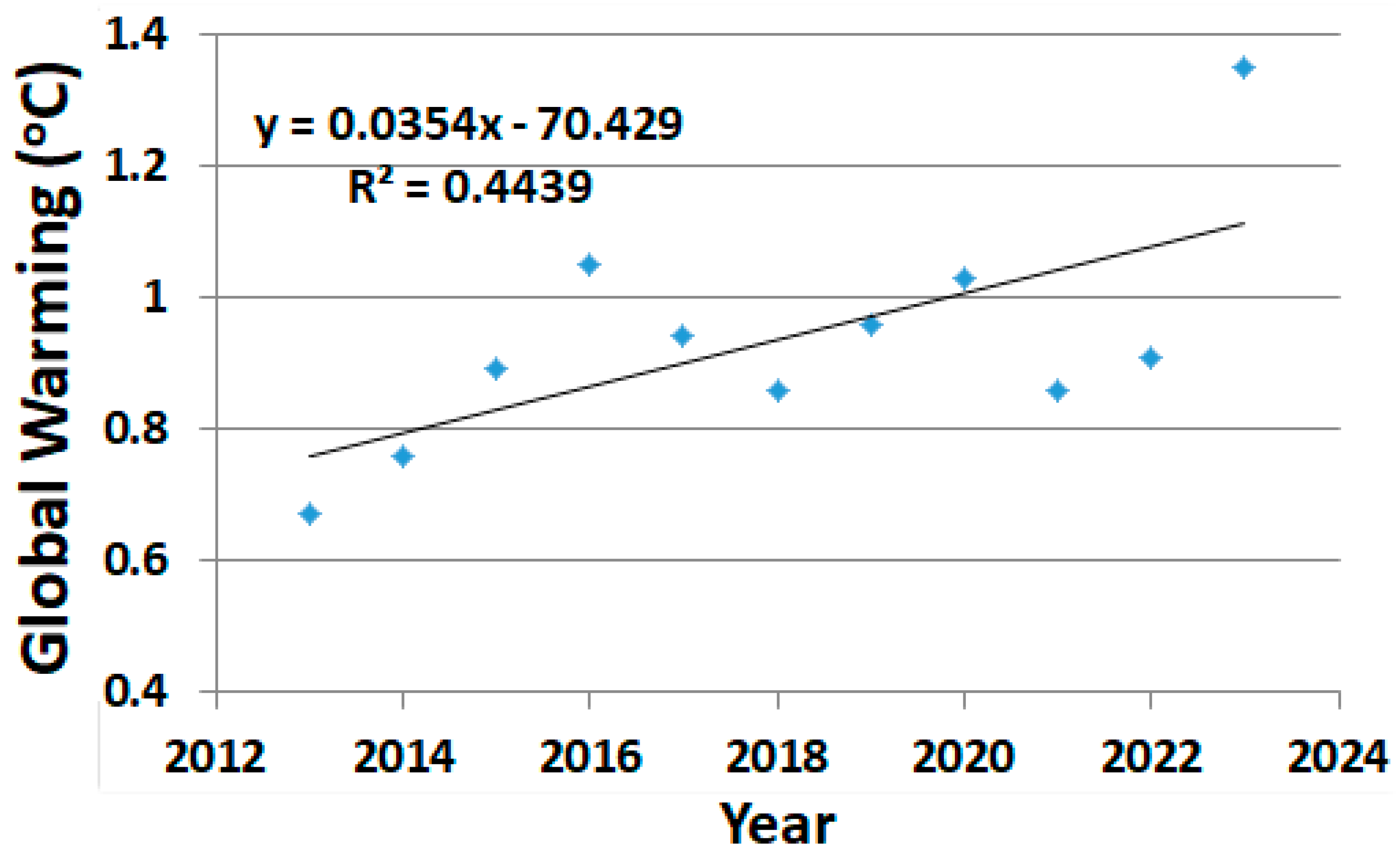
Appendix E. Recent Global Warming 2023 Trend

Figure E1 shows the global warming trend in the last decade, with the large jump in global warming to about 1.35 °C in 2023 [27]. This indicates that the slope appears to have increased from the value of 0.0188 °C/year in Figure 1 to 0.035 °C/year. This is unusual considering that about 0.02 °C/year has been the standard estimate. However, this is influenced by the strong El Niño effect in 2023 and will likely decrease somewhat with the next La Niña effect. Other authors [23] have indicated that a slope of 0.027 °C/year is likely from recent analysis. A 0.027 °C/year increase would lead to a larger annual reversal goal of 0.0419 Wm−2 compared to that used in Equation (6) of 0.029 Wm−2. This is a 45% increase, which would also increase the ASG area requirements proportionately by this amount in Equation (7) and in the results section.
Figure E1. Recent trend in global warming with the 2023 data included.
Climate 12 00026 g0e1

References

  1. Thomson, A.M.; Calvin, K.V.; Smith, S.J.; Kyle, G.P.; Volke, A.; Patel, P.; Delgado-Arias, S.; Bond-Lamberty, B.; Wise, M.A.; Clarke, L.E.; et al. RCP4.5: A pathway for stabilization of radiative forcing by 2100. Clim. Chang. 2011, 109, 77. [Google Scholar] [CrossRef]
  2. Feinberg, A. Urbanization Heat Flux Modeling Confirms it is a Likely Cause of Significant Global Warming: Urbanization Mitigation Requirements. Land 2023, 12, 1222. [Google Scholar] [CrossRef]
  3. Zhang, P.; Ren, G.; Qin, Y.; Zhai, Y.; Zhai, T.; Tysa, S.K.; Xue, X.; Yang, G.; Sun, X. Urbanization effects on estimates of global trends in mean and extreme air temperature. J. Clim. 2021, 34, 1923–1945. [Google Scholar] [CrossRef]
  4. Sánchez, J.; McInnes, C. Optimal Sunshade Configurations for Space-Based Geoengineering near the Sun-Earth L1 Point. PLoS ONE 2015, 10, e0136648. [Google Scholar] [CrossRef] [PubMed]
  5. Early, J. Space-based solar shield to offset greenhouse effect. J. Br. Interplanet. Soc. 1989, 42, 567–569. [Google Scholar]
  6. Govindasamy, B.; Caldeira, K. Geoengineering Earth’s radiation balance to mitigate CO2-induced climate change. Geophys. Res. Lett. 2000, 27, 2141–2144. [Google Scholar] [CrossRef]
  7. Angel, R. Feasibility of cooling the Earth with a cloud of small spacecraft near the inner Lagrange point (L1). Proc. Natl. Acad. Sci. USA 2006, 103, 17184–17189. [Google Scholar] [CrossRef]
  8. Fuglesang, C.; Miciano, M. Realistic sunshade system at L1 for global temperature control. Acta Astronaut. 2021, 186, 269–279. [Google Scholar] [CrossRef]
  9. Bromley, B.; Khan, S.; Kenyon, S. Dust as a solar shield. PLoS Clim. 2023, 2, e0000133. [Google Scholar] [CrossRef]
  10. Jones, A.C.; Haywood, J.M.; Jones, A. Climatic impacts of stratospheric geoengineering with sulfate, black carbon and titania injection. Atmos. Chem. Phys. 2016, 16, 2843–2862. [Google Scholar] [CrossRef]
  11. Tilmes, S.; Sanderson, B.M.; O’Neill, B.C. Climate impacts of geoengineering in a delayed mitigation scenario. Geophys. Res. Lett. 2016, 43, 8222–8229. [Google Scholar] [CrossRef]
  12. Izrael, Y.; Volodin, E.; Kostrykin, S.; Revokatova, A.; Ryaboshapko, A. The ability of stratospheric climate engineering in stabilizing global mean temperatures and an assessment of possible side effects. Atmos. Sci. Lett. 2014, 15, 140–148. [Google Scholar] [CrossRef]
  13. Niemeier, U.; Timmreck, C. What is the limit of climate engineering by stratospheric injection of SO2? Atmos. Chem. Phys. 2015, 15, 9129–9141. [Google Scholar] [CrossRef]
  14. Jones, A.C.; Hawcroft, M.K.; Haywood, J.M.; Jones, A.; Guo, X.; Moore, J.C. Regional Climate Impacts of Stabilizing Global Warming at 1.5 K Using Solar Geoengineering. Earth’s Future 2018, 6, 230–251. [Google Scholar] [CrossRef]
  15. Wigley, T.M. A combined mitigation/geoengineering approach to climate stabilization. Science 2006, 314, 452–454. [Google Scholar] [CrossRef] [PubMed]
  16. Kravitz, B.; Robock, A.; Forster, P.M.; Haywood, J.M.; Lawrence, M.G.; Schmidt, H. An overview of the Geoengineering Model Intercomparison Project (GeoMIP). JGR Atmos. 2013, 118, 13, 103–13, 107. [Google Scholar] [CrossRef]
  17. Barrett, S.; Lenton, T.M.; Millner, A.; Tavoni, A.; Carpenter, S.R.; Anderies, J.M.; Chapin III, F.S.; Crépin, A.S.; Daily, G.; Ehrlich, P.; et al. Climate engineering reconsidered. Nat. Clim. Chang. 2014, 4, 527–529. [Google Scholar] [CrossRef]
  18. Jiang, J.; Cao, L.; MacMartin, D.; Simpson, I.; Kravitz, B.; Cheng, W.; Visioni, D.; Tilmes, S.; Richter, J.; Mills, M. Stratospheric Sulfate Aerosol Geoengineering Could Alter the High-Latitude Seasonal Cycle. Geophys. Res. Lett. 2019, 46, 14153–14163. [Google Scholar] [CrossRef]
  19. Malik, A.; Nowack, P.J.; Haigh, J.D.; Cao, L.; Atique, L.; Plancherel, Y. Tropical Pacific climate variability under solar geoengineering: Impacts on ENSO extremes. Atmos. Chem. Phys. 2020, 20, 15461–15485. [Google Scholar] [CrossRef]
  20. National Academies of Sciences, Engineering, and Medicine. Reflecting Sunlight: Recommendations for Solar Geoengineering Research and Research Governance; Consensus Study Report; National Academies of Sciences, Engineering, and Medicine: Washington, DC, USA, 2021. [Google Scholar] [CrossRef]
  21. Tang, A.; Kemp, L. A Fate Worse Than Warming? Stratospheric Aerosol Injection and Global Catastrophic Risk. Front. Clim. 2021, 3, 720312. [Google Scholar] [CrossRef]
  22. Diffenbaugh, N.; Barnes, E. Data-driven predictions of the time remaining until critical global warming thresholds are reached. Proc. Natl. Acad. Sci. USA 2023, 120, e2207183120. [Google Scholar] [CrossRef]
  23. Hansen, J.E.; Sato, M.; Simons, L.; Nazarenko, L.S.; Sangha, I.; Kharecha, P.; Zachos, J.C.; von Schuckmann, K.; Loeb, N.G.; Osman, M.B.; et al. Global warming in the pipeline. Oxf. Open Clim. Chang. 2023, 3, kgad008. [Google Scholar] [CrossRef]
  24. MEER Project. Mirrors for Earth’s Energy Rebalancing. 2023. Available online: https://www.meer.org/ (accessed on 10 April 2023).
  25. Feinberg, A. Solar Geoengineering Modeling and Applications for Mitigating Global Warming: Assessing Key Parameters and the Urban Heat Island Influence. Front. Clim. 2022, 4, 870071. [Google Scholar] [CrossRef]
  26. NASA Vital Signs. Global Temperature|Vital Signs—Climate Change: Vital Signs of the Planet. 2023. Available online: https://climate.nasa.gov/vital-signs/global-temperature/ (accessed on 10 April 2023).
  27. NOAA. Climate at a Glance Time Series (Land and Ocean Data). Available online: https://www.ncei.noaa.gov/access/monitoring/climate-at-a-glance/global/time-series/globe/ocean/12/12/1975-2023?filter=true&filterType=binomial (accessed on 10 April 2023).
  28. Feinberg, A. A Re-radiation Model for the Earth’s Energy Budget and the Albedo Advantage in Global Warming Mitigation. Dyn. Atmos. Ocean. 2021, 97, 101267. [Google Scholar] [CrossRef]
  29. Hartmann, D.L.; Klein, A.M.G.; Tank, M.; Rusticucci, L.V.; Alexander, S.; Brönnimann, Y.; Charabi, F.J.; Dentener, E.J.; Dlugokencky, D.; Easterling, D.R.; et al. Observations: Atmosphere and Surface. In Climate Change 2013: The Physical Science Basis: Contribution of Working Group I to the Fifth Assessment Report of the Intergovernmental Panel on Climate Change; Stocker, T.F., Qin, D., Plattner, G.-K., Tignor, M., Allen, S.K., Boschung, J., Nauels, A., Xia, Y., Bex, V., Midgley, P.M., Eds.; Cambridge University Press: Cambridge, UK; New York, NY, USA, 2013. [Google Scholar]
  30. Feinberg, A. Climate Sensitivity and Feedback Estimates Using Correlated Rates: Consideration of an Urbanization Influence. 2024. Available online: https://www.researchgate.net/publication/368601957_Climate_sensitivity_and_feedback_estimates_using_correlated_rates_Consideration_of_an_urbanization_influence (accessed on 12 March 2023).
  31. Dessler, A.; Zhan, Z.; Yang, P. Water-vapor climate feedback inferred from climate fluctuations, 2003–2008. Geophys. Res. Lett. 2008, 35, 20. [Google Scholar] [CrossRef]
  32. Liu, R.; Su, H.; Liou, K.; Jiang, J.; Gu, Y.; Liu, S.; Shiu, C. An Assessment of Tropospheric Water Vapor Feedback Using Radiative Kernels. JGR Atmos. 2018, 123, 1499–1509. [Google Scholar] [CrossRef]
  33. Feinberg, A. Urban Heat Island High Water-Vapor Feedback Estimates and Heatwave Issues: A Temperature Difference Approach to Feedback Assessments. Sci 2022, 4, 44. [Google Scholar] [CrossRef]
  34. Feinberg, A. Urban heat island amplification estimates on global warming using an albedo model. SN Appl. Sci. 2020, 2, 2178. [Google Scholar] [CrossRef]
  35. Zhou, D.; Zhao, S.; Zhang, L.; Sun, G.; Liu, Y. The footprint of urban heat island effect in China. Sci. Rep. 2015, 5, 11160. [Google Scholar] [CrossRef] [PubMed]
  36. Smoliak, B.; Gelobter, M.; Haley, J. Mapping potential surface contributions to reflected solar radiation. Environ. Res. Commun. 2022, 4, 065003. [Google Scholar] [CrossRef]
  37. Keutsch, F. The Stratospheric Controlled Perturbation Experiment (SCoPEx); Harvard University: Cambridge, MA, USA, 2020; Available online: https://scopexac.com/wp-content/uploads/2021/03/1.-Scientific-and-Technical-Review-Foundational-Document.pdf (accessed on 10 April 2023).
  38. Keith, D.; Weisenstein, D.; Dykema, J.; Keutsch, F. Stratospheric Solar Geoengineering without Ozone Loss. Proc. Natl. Acad. Sci. USA 2016, 113, 14910–14914. [Google Scholar] [CrossRef]
  39. Tollefson, J. First sun-dimming experiment will test a way to cool the Earth. Nature 2018, 563, 613–615. Available online: https://www.nature.com/articles/d41586-018-07533-4 (accessed on 15 April 2023). [CrossRef]
  40. Ferraro, A.; Charlton-Perez, A.; Highwood, E. Stratospheric dynamics and midlatitude jets under geoengineering with space mirrors and sulfate and titania aerosols. J. Geophys. Res. Atmos. 2015, 120, 414–429. [Google Scholar] [CrossRef]
  41. Dykema, J.; Keith, D.; Anderson, J.; Weisenstein, D. Stratospheric controlled perturbation experiment: A small-scale experiment to improve understanding of the risks of solar geoengineering. Phil. Trans. R. Soc. A 2014, 372, 20140059. [Google Scholar] [CrossRef]
  42. Crutzen, P. Albedo Enhancement by Stratospheric Sulfur Injections: A Contribution to Resolve a Policy Dilemma? Clim. Chang. 2006, 77, 211. [Google Scholar] [CrossRef]
  43. Clifford, C. White House Is Pushing Ahead Research to Cool Earth by Reflecting Back Sunlight. CNBC. 2022. Available online: https://www.cnbc.com/2022/10/13/what-is-solar-geoengineering-sunlight-reflection-risks-and-benefits.html (accessed on 18 September 2023).
  44. Van Vuuren, D.P.; Edmonds, J.; Kainuma, M.; Riahi, K.; Thomson, A.; Hibbard, K.; Hurtt, G.C.; Kram, T.; Kram, V.; Lamarque, J.-F.; et al. The representative concentration pathways: An overview. Clim. Chang. 2011, 109, 5. [Google Scholar] [CrossRef]
  45. Held, M.; Winton, M.; Takahashi, K.; Delworth, T.; Zeng, F. Probing the fast and slow components of global warming by returning abruptly to preindustrial forcing. J. Clim. 2010, 23, 2418–2427. [Google Scholar] [CrossRef]
  46. Wikipedia. List of Countries by Total Wealth. 2022. Available online: https://en.wikipedia.org/wiki/List_of_countries_by_total_wealth (accessed on 17 September 2023).
  47. Mautner, M.N. A space-based solar screen against climatic warming. J. Br. Interplanet. Soc. 1991, 44, 135–138. [Google Scholar]
  48. Maghazel, O.; Netland, T. Drones in manufacturing: Exploring opportunities for research and practice. J. Manuf. Technol. Manag. 2019, 31, 1237–1259. [Google Scholar] [CrossRef]
  49. Klauser, F.; Pauschinger, D. Entrepreneurs of the air: Sprayer drones as mediators of volumetric agriculture. J. Rural Stud. 2021, 84, 55–62. [Google Scholar] [CrossRef]
  50. Agri Spray Drones. How Many Acres per Hour or Day Can a Spray Drone Spray? Available online: https://agrispraydrones.com/how-many-acres-per-hour-or-day-can-a-spray-drone-spray/ (accessed on 9 June 2023).
  51. Li, X.; Peoples, J.; Yao, P.; Ruan, X. Ultrawhite BaSO4 Paints and Films for Remarkable Daytime Subambient Radiative Cooling. ACS Appl. Mater. Interfaces 2021, 13, 21733–21739. [Google Scholar] [CrossRef]
  52. Felicelli, A.; Katsamba, I.; Barrios, F.; Zhang, Y.; Guo, Z.; Peoples, J.; Chiu, G.; Ruan, X. Thin layer lightweight and ultrawhite hexagonal boron nitride nanoporous paints for daytime radiative cooling. Cell Rep. Phys. Sci. 2022, 3, 101058. [Google Scholar] [CrossRef]
  53. Grossman, D. With Sawdust and Paint, Locals Fight to Save Peru’s Glaciers. 2012. Available online: https://theworld.org/stories/2012-09-25/sawdust-and-paint-locals-fight-save-perus-glaciers (accessed on 3 March 2023).
  54. Huang, X.; Yang, J.; Wang, W.; Liu, Z. Mapping 10 m global impervious surface area (GISA-10m) using multi-source geospatial data. Earth Syst. Sci. Data 2022, 14, 3649–3672. [Google Scholar] [CrossRef]
  55. Sun, Z.; Du, W.; Jiang, H.; Weng, Q.; Guo, H.; Han, Y.; Xing, Q.; Ma, Y. Global 10-m impervious surface area mapping: A big earth data based extraction and updating approach. Int. J. Appl. Earth Obs. Geoinf. 2022, 109, 102800. [Google Scholar] [CrossRef]
  56. Azari Jafari, H.; Kirchain, R.; Gregory, J. Mitigating Climate Change with Reflective Pavements. MIT Study on Roads. CSHub Topic Summary. 2020. Available online: https://cshub.mit.edu/sites/default/files/images/Albedo%201113_0.pdf (accessed on 25 November 2022).
  57. Wikipedia. Gasoline Gallon Equivalent. 2021. Available online: https://en.wikipedia.org/wiki/Gasoline_gallon_equivalent (accessed on 4 December 2021).
  58. Ong, S.; Campbell, C.; Denholm, P.; Magolis, R.; Heath, G. Land-Use Requirements for Solar Power Plants in the United States; Technical Report NREL/TP-6A20-56290; National Renewable Energy Lab. (NREL): Golden, CO, USA, 2013. Available online: https://www.nrel.gov/docs/fy13osti/56290.pdf (accessed on 11 November 2023).
  59. Zhao, L.; Lee, X.; Smith, R.; Oleson, K. Strong, contributions of local background climate to urban heat islands. Nature 2014, 511, 216–219. [Google Scholar] [CrossRef] [PubMed]
  60. EPA. Study Cambridge Systematics. Cool Pavement Report, Heat Island Reduction Initiative. 2005. Available online: https://citeseerx.ist.psu.edu/viewdoc/download?doi=10.1.1.648.3147&rep=rep1&type=pd (accessed on 12 March 2023).
  61. Smart Surfaces Coalition. Available online: https://smartsurfacescoalition.org/smart-surfaces (accessed on 12 March 2023).
  62. ScienceDirect, Calcium Carbonate. Available online: https://www.sciencedirect.com/topics/chemistry/calcium-carbonate (accessed on 23 April 2023).
  63. AmericanElements, Calcium Carbonate Nanoparticles. Available online: https://www.americanelements.com/calcium-carbonate-nanoparticles-471-34-1#:~:text=About%20Calcium%20Carbonate%20Nanoparticles,60%20m2%2Fg%20range (accessed on 23 April 2023).
  64. Urupina, D.; Lasne, J.; Romanias, M.N.; Thiery, V.; Dagsson-Waldhauserova, P.; Thevenet, F. Uptake and surface chemistry of SO2 on natural volcanic dusts. Atmos. Environ. 2019, 217, 116942. [Google Scholar] [CrossRef]
  65. Forster, P.; Storelvmo, T.; Armour, K.; Collins, W.; Dufresne, J.L.; Frame, D.; Lunt, D.J.; Mauritsen, T.; Palmer, M.D.; Watanabe, M.; et al. The Earth’s Energy Budget, Climate Feedbacks, and Climate Sensitivity. In Climate Change 2021: The Physical Science Basis: Contribution of Working Group I to the Sixth Assessment Report of the Intergovernmental Panel on Climate Change; Masson-Delmotte, V., Zhai, P., Pirani, A., Connors, S.L., Péan, C., Berger, S., Caud, N., Chen, Y., Goldfarb, L., Gomis, M.I., et al., Eds.; Cambridge University Press: Cambridge, UK; New York, NY, USA, 2023; pp. 923–1054. [Google Scholar] [CrossRef]
Figure 2. Global warming (a) over land and (b) over the ocean [27].
Climate 12 00026 g002
Table 1. ASG overview by section.
ObjectiveSectionHighlighted ResultsOther
Reference(s)
ASG temperature reversal2.2, Equation (1)−0.0188 °C/year
This is the estimated yearly temperature reversal goal.
NASA [26]; NOAA [27]
ASG energy reversal2.3, Equation (6)−0.0293 Wm−2/year
This is the estimated yearly reverse forcing requirement to achieve the temperature reversal.
Findings,
Feinberg [25]
SG savings and greenhouse gas equivalency 2.3.1Results indicate an estimated 38% work saving for climate mitigation using SG compared to CDR.Feinberg
[28], Findings
SRM area estimate equation 2.3.2 Δ P A S G = S o 4 A T A E X C X O X S H T ( Δ α T )
SRM area estimates can be determined using this equation.
Findings,
Feinberg [25]
Earth brightening transmission loss3.1The probability of clear sky transmission is 78%.
This helps to provide estimates since not all of the SRM reflected radiation escapes to outer space.
Findings
Earth brightening
cool pavement example
3.1.1 A T A E = 0.078 % p e r y e a r B a y e s 0.0612 % p e r y e a r M i n i m u m
AT is the area modification relative to the area of the Earth AE
Findings
L1 Space sunshade estimates3.2 A T A E = 0.003 % p e r y e a r
This is the required area for a space disc at L1
Findings
Annual stratospheric injection estimates3.3Table 3, 0.313 Mt[SO2]Yr−1
This is the amount of SO2 injection per year for ASG
Findings
Overview of estimates3.4Table 4 and Table 5 provide a concise summary of the area requirements for different SRM methodsFindings
RCP ASG cumulative area estimates3.5ASG cumulative estimates anticipated with different RCP scenariosFindings
ASR management—recommendations4.1.1, 4.1.2, 4.1.3, 4.1.4, 4.1.5, 4.1.64.1.1: Allocation by country
4.1.2: L1 Space clusters
4.1.3 Earth brightening
4.1.4: Natural hotspots
4.1.5: Mixed planning and ratings
4.1.6: Negative SG
Findings
Conclusions5 Findings
Earth brightening of hotspots and water vapor feedbackAppendix A Δ P A S G = 0.0147   Wm 2 / Yr .
The results find that feedback reductions can be increased in some hotspot areas, further reducing the SRM area. In this example, the SG goal is cut in half.
Findings
Bayesian estimate for outgoing transmission Appendix BTrClear = 1 − 0.22 = 0.78
This is the Bayes estimate for the probability of the reflected sunlight from an SRM area to reach outer space.
Findings
CaCO3 and SO2 stratospheric injections—area approachAppendix C A T A E = 0.0288 % / eff
This is the area coverage estimated for these aerosols and depends on their reflection efficiencies.
Findings
Feedback conversionsAppendix DConverts feedback amplification to feedback units.Estimates
Recent GW 2023 trendsAppendix ERecent trends due to a 2023 GW jumpEstimates
SG calculatorSupplementary MaterialsSG helpful calculator is provided for the results.Findings
Table 2. Symbol definitions.
SymbolDefinition
A T Target area: This is the area for which an SRM albedo modification is to be applied
A E Earth’s area
AFFeedback amplification with average taken as AF = 2.15: A unit less number, to convert to feedback units see Appendix D
CCClausius–Clapeyron relation
α T , α T SG target’s albedo modification: α T is before, α T is after SRM (Equations (7) and (8))
f = 62%Re-radiation factor: Average re-radiation occurring in the atmosphere
HTUHI microclimate amplification factor
I S O 2 SO2 injection rate
Δ R T O A Radiation change at the TOA
∆PASGAnnual reversal in Watts/m2: Reverse forcing to mitigate annual yearly increase in GW (this does not include feedback which is assumed to reverse the amount required
∆PRevReversal change in Watts/m2: Full GW reversal required (includes reverse forcing and feedback)
Δ P T Reverse forcing albedo change from a target area T in Watts/m2: This is the reverse forcing required assuming the feedback portion would also reverse
S o / 4 Average solar radiation S o / 4 = 340.25 Wm 2
TRTemperature reversal: ASG goal to reverse this temperature rise (Equation (1))
TRTransmissibility: This is applied to a small reduction in the incoming solar radiation from the sun (1361 Wm−2)
TOATop of the atmosphere
XSSolar irradiance averaging 47%
XSSpace irradiance: If at L1 in space, XS = 4, if in other areas, XS = 1
Table 3. SO2 injection requirements for SRM.
Stratosphere InjectionFull
Reversal
Annual
Reversal
ΔRTOA (Wm−2)1.470.0293
I S O 2 (Mt[SO2]Yr−1)6.850.313
Savings5.7 *22 **
* Saving relative to a goal of 5.1 Wm−2; ** = 6.85/0.313
Table 4. ASG requirements for land and space.
Earth BrighteningSpace
ParametersPavements
Roofs
Desert TreatmentUHIsEarth
(Sea)
Mirrors **
L1 Space Sunshading ParametersStratosphere
Injections
∆PASG (Wm−2)−0.0293−0.0293−0.0293−0.0293∆PASG (Wm−2)−0.0293−0.0293
XS = 1, XO = 1, XC =0.470.920.470.7 (0.85)XC = 1, XS =41
Δ α T 0.30.440.10.75 Δ α T 0.70.3
HT1132 (1)HT11
A ¯ F 2.152.152.152.15 A ¯ F 2.152.15
Earth Brightening Minimal ResultsL1 Space Disc ResultsSO2, CaCO3 Injec.
AT/AE0.061%0.0212%0.062%0.0082%
(0.0144%)
AT/AE Earth Shade0.00308%0.0288%/eff
(0.31 Mt[SO2]Yr−1)
AT (Mi2)120,07041,880120,07016,122
(28,350)
Shade AT (Mi2, km2)6046, 15,58655,848, 148,644
Radius (Mi)19611519672 (95)Shade Radius (Mi, km)43, 71133, 218
AT (km2)3.1 × 1051.08 × 1053.1 × 1054.2 × 104
(7.3 × 10⁴)
Disc Area (Mi2, km2) *6046, 15,586-
Radius (km)315131315116 (153)Disc Radius (Mi, km) *43, 71-
* Depends on the Sun-blocking efficiency of the disc and actual distance relative to L1. ** Sea mirrors are usually expected to be floating reflective particles or objects.
Table 5. ASG potential hotspot possible requirements.
T2, T1
Δ α T XC
61 °C, 33 °C
0.5, 0.47
AF4.3
ΔPASG (Wm−2)−0.0293
AT/AE0.0184%
AT (Mi2)36,022
Radius (Mi)107
AT (km2)0.9 × 10⁵
Radius (km)169
Table 6. Cumulative ASG area estimates for different RCP scenarios with a 10-year time lag.
RCP
Scenarios
Peak Year,
(CO2 ppm)
Peak Plus 10-Year Lag for ASG
(Starting in 2023)
Years
Earth Surface
Brightening *
AT/AE
L1 Space Disc Size *
AT/AE
I S O 2 *
(Mt[SO2]Yr−1)
RCP 2.62025 (430 ppm)120.061% × 12 = 0.73%0.003% × 12 = 0.036%0.313 × 12 = 3.8
RCP 4.52045 (475 ppm)320.061% × 32 = 1.95%0.003% × 32 = 0.1%0.313 × 32 = 10
* See Table 4.
Table 7. Author ratings for ASG SRM methods (ratings 1–10, 1 is best, 10 is worst).
ASG SRM MethodCost RatingPolitical-Governance RatingLikely
Success Rating
Main-
Tenance
Cost
Average RatingKey IssuesUS Agencies That May Be Involved *
Earth Brightening11–4
(4 for SRM of natural hotspot)
332.0–2.8Will require technological advances in AI drones for many paint applicationsDOT, NASA, Space-X, city building codes
SAI596107.5Highly politicalNASA, Space-X
L1 Space Mirrors1031–33–54.3–5.3High costs and difficultyNASA, Space-X
L1 Moon Dust942–7106.3–7.5High costs and difficultyNASA, Space-X
Mixed Method54.535.54.5Same as aboveSame as above
* Will require similar agencies in other countries.
Disclaimer/Publisher’s Note: The statements, opinions and data contained in all publications are solely those of the individual author(s) and contributor(s) and not of MDPI and/or the editor(s). MDPI and/or the editor(s) disclaim responsibility for any injury to people or property resulting from any ideas, methods, instructions or products referred to in the content.

