


Impacts of Climate Change in Baja California Winegrape Yield


 ,
,  and
and 
Abstract
1. Introduction
2. Data and Methods
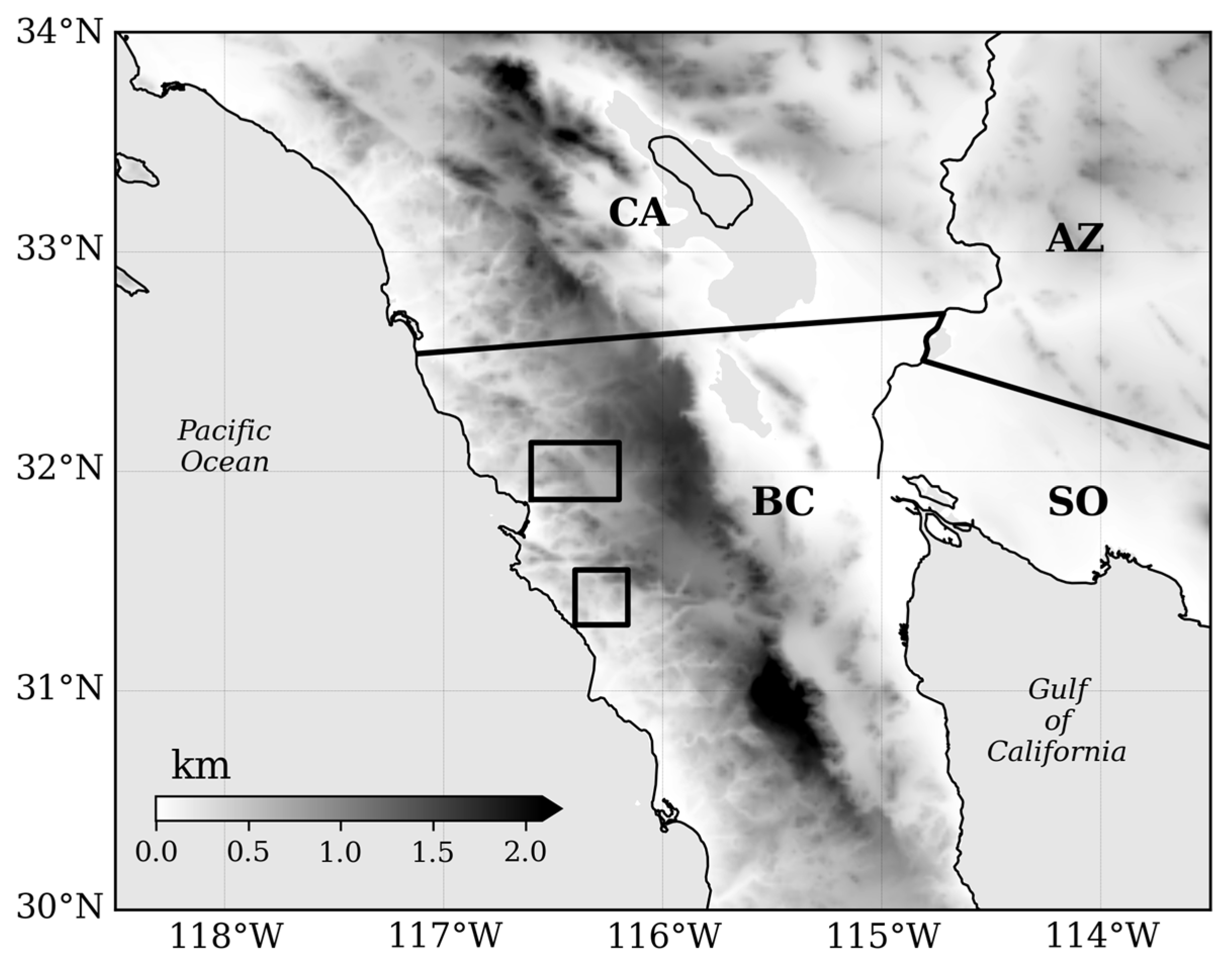
2.1. Study Region
2.2. Data
2.2.1. Climatic Data
2.2.2. Economic Data
2.2.3. Climate Change Scenarios
2.3. Method
2.3.1. Regional Climate
2.3.2. Regression Model
3. Results
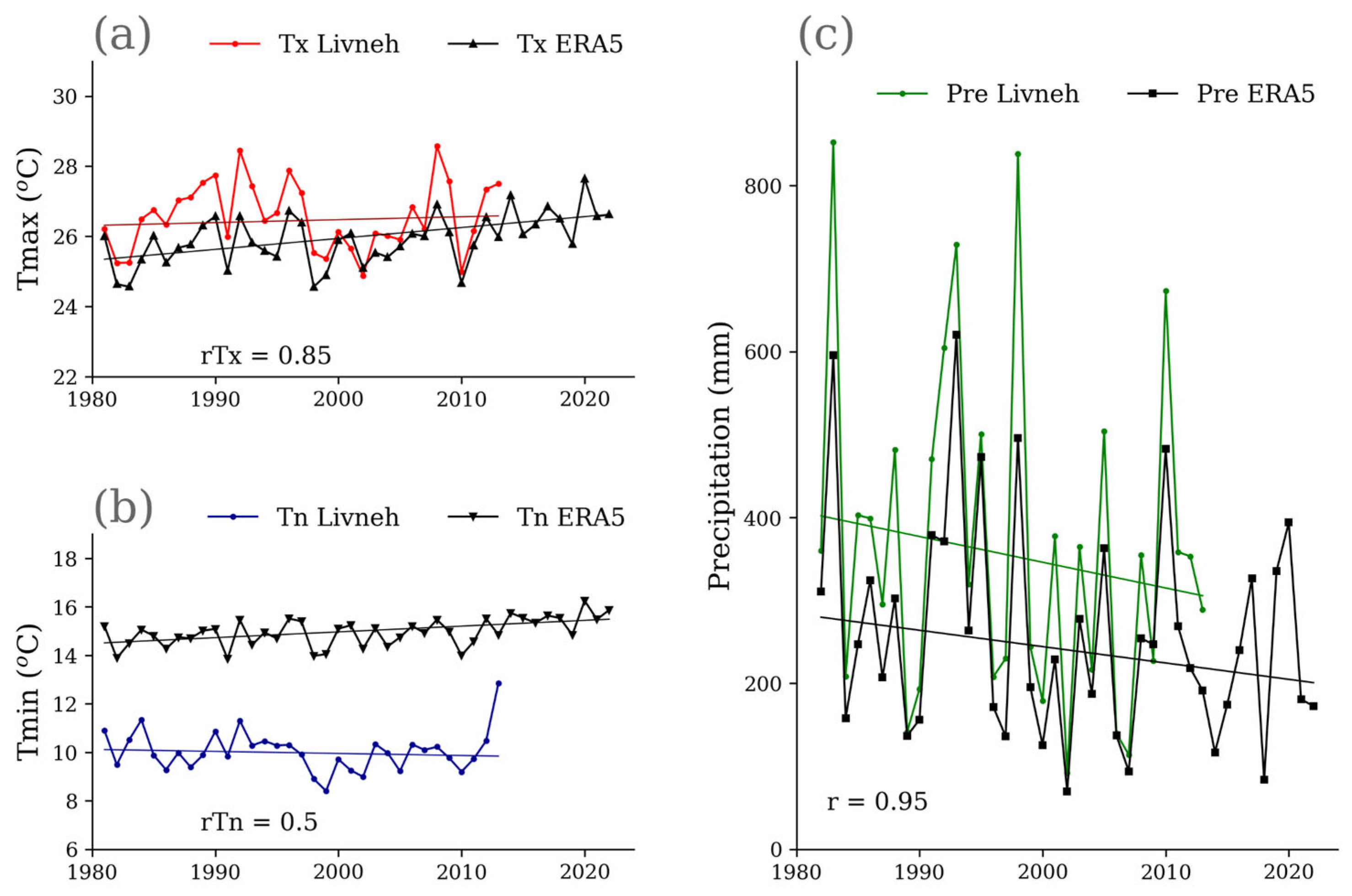
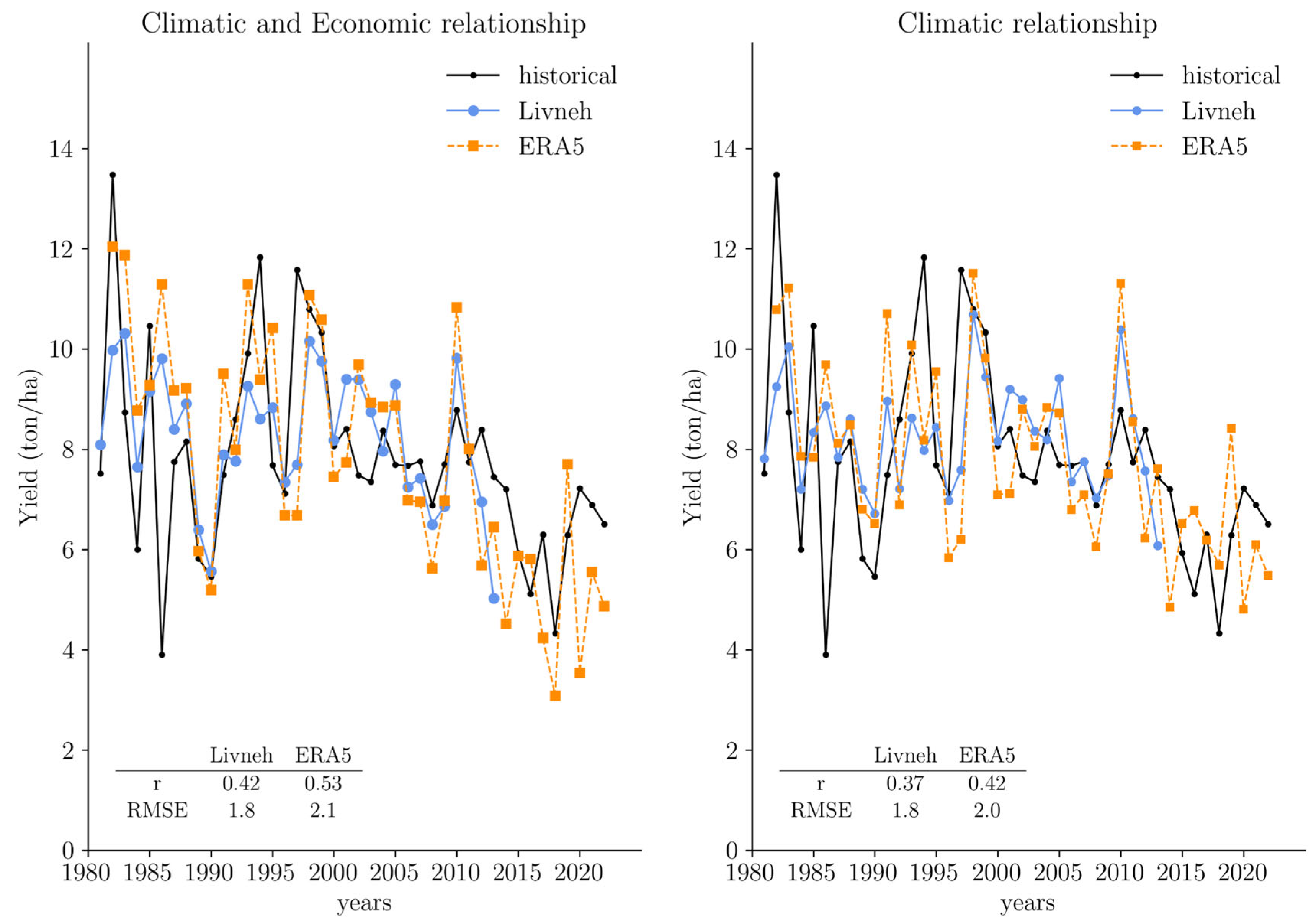
3.1. Climate Characteristics and Regression Models
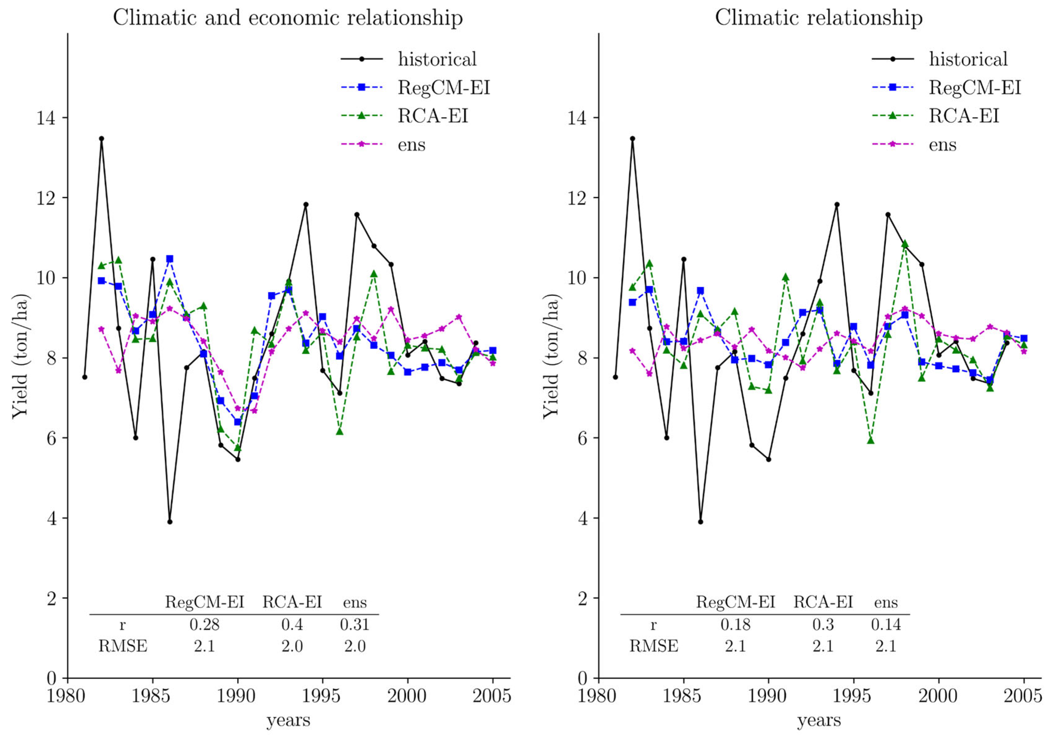
3.2. Seasonal Climatic Conditions with the Ensemble of RCMs
3.3. Regional Climate Change Scenarios
3.4. Winegrape Yield According to Climate Change Scenarios
4. Discussion and Conclusions
Author Contributions
Funding
Data Availability Statement
Acknowledgments
Conflicts of Interest
References
- Castillo, N.; Cavazos, T.; Pavia, E. Impact of Climate Change in Mexican Winegrape Regions. Int. J. Climatol. 2023, 43, 6621–6642. [Google Scholar] [CrossRef]
- CMV. Plan Rector—Consejo Mexicano Vitivinícola; Secretaría de Agricultura, Ganadería, Desarrollo Rural, Pesca y Alimentación: Ciudad de Mexico, Mexico, 2018; p. 92. [Google Scholar]
- Servicio de Información Agroalimentaria y Pesquera—SIAP. Panorama Agroalimentario 2021; Secretaría de Agricultura, Ganadería, Desarrollo Rural, Pesca y Alimentación: Ciudad de Mexico, Mexico, 2021; p. 200. [Google Scholar]
- Servicio de Información Agroalimentaria y Pesquera—SIAP. Panorama Agroalimentario 2022; Secretaría de Agricultura, Ganadería, Desarrollo Rural, Pesca y Alimentación: Progreso, Mexico, 2022; p. 218. [Google Scholar]
- Reyes-Orta, M.; Olague, J.T.; Lobo Rodriguez, M.O.; Cruz Estrada, I. Importance and Valuation of the Components of Satisfaction in the Oenological Experience in Guadalupe Valley Ensenada, Baja California: Contributions to the Process of Sustainable Management. Rev. Análisis Turístico 2016, 22, 39–55. [Google Scholar]
- IPCC. Climate Change 2021—The Physical Science Basis; Contribution of Working Group I to the Sixth Assessment Report of the Intergovernmental Panel on Climate Change; Cambridge University Press: Cambridge, UK; New York, NY, USA, 2021; p. 2391. [CrossRef]
- Jones, G.V.; Goodrich, G.B. Influence of Climate Variability on Wine Regions in the Western USA and on Wine Quality in the Napa Valley. Clim. Res. 2008, 35, 241–254. [Google Scholar] [CrossRef]
- Jones, G.V.; Reid, R.; Vilks, A. Climate, Grapes, and Wine: Structure and Suitability in a Variable and Changing Climate. In The Geography of Wine: Regions, Terroir and Techniques; Springer: Dordrecht, The Netherlands, 2012; pp. 109–133. [Google Scholar] [CrossRef]
- Riekötter, N.; Hassler, M. Agroforestry Systems in Wine Production-Mitigating Climate Change in the Mosel Region. Forests 2022, 13, 1755. [Google Scholar] [CrossRef]
- Trejo-Pech, C.O.; Arellano-Sada, R.; Coelho, A.M.; Weldon, R.N. Is the Baja California, Mexico, Wine Industry a Cluster? Am. J. Agric. Econ. 2012, 94, 569–575. [Google Scholar] [CrossRef]
- Winkler, A.J. General Viticulture; University of California Press: Berkeley, CA, USA, 1974. [Google Scholar]
- Vaudour, E. The Quality of Grapes and Wine in Relation to Geography: Notions of Terroir at Various Scales. J. Wine Res. 2002, 13, 117–141. [Google Scholar] [CrossRef]
- Cramer, W.; Guiot, J.; Fader, M.; Garrabou, J.; Gattuso, J.-P.; Iglesias, A.; Lange, M.A.; Lionello, P.; Llasat, M.C.; Paz, S. Climate Change and Interconnected Risks to Sustainable Development in the Mediterranean. Nat. Clim. Chang. 2018, 8, 972–980. [Google Scholar] [CrossRef]
- IPCC. Climate Change 2023: Synthesis Report; Lee, H., Romero, J., Eds.; Contribution of Working Groups I, II and III to the Sixth Assessment Report of the Intergovernmental Panel on Climate Change; IPCC: Geneva, Switzerland, 2023; p. 184. [CrossRef]
- Romero Azorin, P.; Garcia Garcia, J. The Productive, Economic, and Social Efficiency of Vineyards Using Combined Drought-Tolerant Rootstocks and Efficient Low Water Volume Deficit Irrigation Techniques under Mediterranean Semiarid Conditions. Sustainability 2020, 12, 1930. [Google Scholar] [CrossRef]
- Santillán, D.; Iglesias, A.; La Jeunesse, I.; Garrote, L.; Sotes, V. Vineyards in Transition: A Global Assessment of the Adaptation Needs of Grape Producing Regions under Climate Change. Sci. Total Environ. 2019, 657, 839–852. [Google Scholar] [CrossRef]
- Santillán, D.; Garrote, L.; Iglesias, A.; Sotes, V. Climate Change Risks and Adaptation: New Indicators for Mediterranean Viticulture. Mitig. Adapt. Strateg. Glob. Chang. 2020, 25, 881–899. [Google Scholar] [CrossRef]
- Covarrubias, J.; Thach, L. Wines of Baja Mexico: A Qualitative Study Examining Viticulture, Enology, and Marketing Practices. Wine Econ. Policy 2015, 4, 110–115. [Google Scholar] [CrossRef]
- Nemani, R.R.; White, M.A.; Cayan, D.R.; Jones, G.V.; Running, S.W.; Coughlan, J.C.; Peterson, D.L. Asymmetric Warming over Coastal California and Its Impact on the Premium Wine Industry. Clim. Res. 2001, 19, 25–34. [Google Scholar] [CrossRef]
- Cabello-Pasini, A.; Macias-Carranza, V.; Mejía-Trejo, A. Efecto Del Mesoclima En La Maduración de Uva Nebbiolo (Vitis Vinifera) En El Valle de Guadalupe, Baja California, México. Agrociencia 2017, 51, 617–633. [Google Scholar]
- Asatryan, H.; Aleksanyan, V.; Azatyan, L.; Manucharyan, M. Dynamics of the Development of Viticulture in RA: The Econometric Case Study. Stat. J. IAOS 2022, 38, 1461–1471. [Google Scholar] [CrossRef]
- Markopoulos, T.; Stougiannidou, D.; Kontakos, S.; Staboulis, C. Wine Quality Control Parameters and Effects of Regional Climate Variation on Sustainable Production. Sustainability 2023, 15, 3512. [Google Scholar] [CrossRef]
- OECD/FAO. OECD-FAO Agricultural Outlook 2023–2032; OECD Publishing: Paris, France, 2023. [Google Scholar] [CrossRef]
- De Orduna, R.M. Climate Change Associated Effects on Grape and Wine Quality and Production. Food Res. Int. 2010, 43, 1844–1855. [Google Scholar] [CrossRef]
- Mori, K.; Goto-Yamamoto, N.; Kitayama, M.; Hashizume, K. Loss of Anthocyanins in Red-Wine Grape under High Temperature. J. Exp. Bot. 2007, 58, 1935–1945. [Google Scholar] [CrossRef] [PubMed]
- White, M.A.; Diffenbaugh, N.; Jones, G.V.; Pal, J.; Giorgi, F. Extreme Heat Reduces and Shifts United States Premium Wine Production in the 21st Century. Proc. Natl. Acad. Sci. USA 2006, 103, 11217–11222. [Google Scholar] [CrossRef]
- Camps, J.O.; Ramos, M.C. Grape Harvest and Yield Responses to Inter-Annual Changes in Temperature and Precipitation in an Area of North-East Spain with a Mediterranean Climate. Int. J. Biometeorol. 2012, 56, 853–864. [Google Scholar] [CrossRef]
- Cook, B.I.; Wolkovich, E.M. Climate Change Decouples Drought from Early Wine Grape Harvests in France. Nat. Clim. Chang. 2016, 6, 715–719. [Google Scholar] [CrossRef]
- Duchêne, E.; Huard, F.; Dumas, V.; Schneider, C.; Merdinoglu, D. The Challenge of Adapting Grapevine Varieties to Climate Change. Clim. Res. 2010, 41, 193–204. [Google Scholar] [CrossRef]
- Ferrise, R.; Trombi, G.; Moriondo, M.; Bindi, M. Climate Change and Grapevines: A Simulation Study for the Mediterranean Basin. J. Wine Econ. 2016, 11, 88–104. [Google Scholar] [CrossRef]
- Hannah, L.; Roehrdanz, P.R.; Ikegami, M.; Shepard, A.V.; Shaw, M.R.; Tabor, G.; Zhi, L.; Marquet, P.A.; Hijmans, R.J. Climate Change, Wine, and Conservation. Proc. Natl. Acad. Sci. USA 2013, 110, 6907–6912. [Google Scholar] [CrossRef] [PubMed]
- Jones, G.; Duchêne, E.; Tomasi, D.; Yuste, J.; Braslavska, O.; Schultz, H.; Martinez, C.; Boso, S.; Langellier, F.; Perruchot, C. Changes in European Winegrape Phenology and Relationships with Climate. In Proceedings of the XIV International GESCO Viticulture Congress, Geisenheim, Germany, 23–27 August 2005; pp. 54–61. [Google Scholar]
- Santillán, D.; Sotés, V.; Iglesias, A.; Garrote, L. Adapting Viticulture to Climate Change in the Mediterranean Region: Evaluations Accounting for Spatial Differences in the Producers-Climate Interactions. BIO Web Conf. 2019, 12, 01001. [Google Scholar] [CrossRef]
- Schultz, H.R.; Jones, G.V. Climate Induced Historic and Future Changes in Viticulture. J. Wine Res. 2010, 21, 137–145. [Google Scholar] [CrossRef]
- Van Leeuwen, C.; Darriet, P. The Impact of Climate Change on Viticulture and Wine Quality. J. Wine Econ. 2016, 11, 150–167. [Google Scholar] [CrossRef]
- SEFOA. Panorama General de Valle de Guadalupe, Baja California, 2015; SAGARPA: Tijuana, Mexico, 2015; p. 18. [Google Scholar]
- CONAGUA. Atlas del Agua en México 2018; SEMARNAT: León, Mexico, 2015; p. 143.
- Arriaga-Ramírez, S.; Cavazos, T. Regional Trends of Daily Precipitation Indices in Northwest Mexico and Southwest United States. J. Geophys. Res. Atmos. 2010, 115, D14. [Google Scholar] [CrossRef]
- Cavazos, T.; Rivas, D. Variability of Extreme Precipitation Events in Tijuana, Mexico. Clim. Res. 2004, 25, 229–243. [Google Scholar] [CrossRef]
- SEFOA. Estudio Estadístico Sobre La Producción de Uva En Baja California; SAGARPA: Tijuana, Mexico, 2011; p. 37. [Google Scholar]
- Livneh, B.; Bohn, T.J.; Pierce, D.W.; Munoz-Arriola, F.; Nijssen, B.; Vose, R.; Cayan, D.R.; Brekke, L. A Spatially Comprehensive, Hydrometeorological Data Set for Mexico, the US, and Southern Canada 1950–2013. Sci. Data 2015, 2, 150042. [Google Scholar] [CrossRef]
- Hersbach, H.; Bell, B.; Berrisford, P.; Hirahara, S.; Horányi, A.; Muñoz-Sabater, J.; Nicolas, J.; Peubey, C.; Radu, R.; Schepers, D. The ERA5 Global Reanalysis. Q. J. R. Meteorol. Soc. 2020, 146, 1999–2049. [Google Scholar] [CrossRef]
- Muñoz-Sabater, J.; Dutra, E.; Agustí-Panareda, A.; Albergel, C.; Arduini, G.; Balsamo, G.; Boussetta, S.; Choulga, M.; Harrigan, S.; Hersbach, H. ERA5-Land: A State-of-the-Art Global Reanalysis Dataset for Land Applications. Earth Syst. Sci. Data 2021, 13, 4349–4383. [Google Scholar] [CrossRef]
- Dee, D.P.; Uppala, S.M.; Simmons, A.J.; Berrisford, P.; Poli, P.; Kobayashi, S.; Andrae, U.; Balmaseda, M.; Balsamo, G.; Bauer, d.P. The ERA-Interim Reanalysis: Configuration and Performance of the Data Assimilation System. Q. J. R. Meteorol. Soc. 2011, 137, 553–597. [Google Scholar] [CrossRef]
- Cavazos, T.; Luna-Niño, R.; Cerezo-Mota, R.; Fuentes-Franco, R.; Méndez, M.; Pineda Martínez, L.F.; Valenzuela, E. Climatic Trends and Regional Climate Models Intercomparison over the CORDEX-CAM (Central America, Caribbean, and Mexico) Domain. Int. J. Climatol. 2020, 40, 1396–1420. [Google Scholar] [CrossRef]
- Giorgi, F.; Coppola, E.; Solmon, F.; Mariotti, L.; Sylla, M.; Bi, X.; Elguindi, N.; Diro, G.; Nair, V.; Giuliani, G. RegCM4: Model Description and Preliminary Tests over Multiple CORDEX Domains. Clim. Res. 2012, 52, 7–29. [Google Scholar] [CrossRef]
- Samuelsson, P.; Jones, C.G.; Willén, U.; Ullerstig, A.; Gollvik, S.; Hansson, U.; Jansson, E.; Kjellström, C.; Nikulin, G.; Wyser, K. The Rossby Centre Regional Climate Model RCA3: Model Description and Performance. Tellus A Dyn. Meteorol. Oceanogr. 2011, 63, 4–23. [Google Scholar] [CrossRef]
- Giorgi, F.; Jones, C.; Asrar, G.R. Addressing Climate Information Needs at the Regional Level: The CORDEX Framework. World Meteorol. Organ. (WMO) Bull. 2009, 58, 175. [Google Scholar]
- Giorgi, F.; Gutowski, W.J., Jr. Regional Dynamical Downscaling and the CORDEX Initiative. Annu. Rev. Environ. Resour. 2015, 40, 467–490. [Google Scholar] [CrossRef]
- Collins, W.; Bellouin, N.; Doutriaux-Boucher, M.; Gedney, N.; Halloran, P.; Hinton, T.; Hughes, J.; Jones, C.; Joshi, M.; Liddicoat, S. Development and Evaluation of an Earth-System Model–HadGEM2. Geosci. Model Dev. 2011, 4, 1051–1075. [Google Scholar] [CrossRef]
- Giorgetta, M.A.; Jungclaus, J.; Reick, C.H.; Legutke, S.; Bader, J.; Böttinger, M.; Brovkin, V.; Crueger, T.; Esch, M.; Fieg, K.; et al. Climate and Carbon Cycle Changes from 1850 to 2100 in MPI-ESM Simulations for the Coupled Model Intercomparison Project Phase 5. J. Adv. Model Earth Syst. 2013, 5, 572–597. [Google Scholar] [CrossRef]
- Dunne, J.P.; John, J.G.; Adcroft, A.J.; Griffies, S.M.; Hallberg, R.W.; Shevliakova, E.; Stouffer, R.J.; Cooke, W.; Dunne, K.A.; Harrison, M.J. GFDL’s ESM2 Global Coupled Climate–Carbon Earth System Models. Part I: Physical Formulation and Baseline Simulation Characteristics. J. Clim. 2012, 25, 6646–6665. [Google Scholar] [CrossRef]
- Lobell, D.B.; Field, C.B.; Cahill, K.N.; Bonfils, C. Impacts of Future Climate Change on California Perennial Crop Yields: Model Projections with Climate and Crop Uncertainties. Agric. For. Meteorol. 2006, 141, 208–218. [Google Scholar] [CrossRef]
- González Andrade, S.; Fuentes Flores, N. Matriz de Insumo Producto Vitivinícola de Baja California México. Rev. Econ. 2013, 30, 57. [Google Scholar] [CrossRef]
- González Andrade, S. Cadena de Valor Económico Del Vino de Baja California, México. Estud. Front. 2015, 16, 163–193. [Google Scholar] [CrossRef]
- Gay, C.; Estrada, F.; Conde, C.; Eakin, H.; Villers, L. Potential Impacts of Climate Change on Agriculture: A Case of Study of Coffee Production in Veracruz, Mexico. Clim. Chang. 2006, 79, 259–288. [Google Scholar] [CrossRef]
- Lobell, D.B.; Cahill, K.N.; Field, C.B. Historical Effects of Temperature and Precipitation on California Crop Yields. Clim. Chang. 2007, 81, 187–203. [Google Scholar] [CrossRef]
- Shrestha, N. Detecting Multicollinearity in Regression Analysis. Am. J. Appl. Math. Stat. 2020, 8, 39–42. [Google Scholar] [CrossRef]
- Sen, P.K. Estimates of the Regression Coefficient Based on Kendall’s Tau. J. Am. Stat. Assoc. 1968, 63, 1379–1389. [Google Scholar] [CrossRef]
- Kendall, M.G. Rank Correlation Methods; Griffin: London, UK, 1948. [Google Scholar]
- Colorado-Ruiz, G.; Cavazos, T.; Salinas, J.A.; De Grau, P.; Ayala, R. Climate Change Projections from Coupled Model Intercomparison Project Phase 5 Multi-model Weighted Ensembles for Mexico, the North American Monsoon, and the Mid-summer Drought Region. Int. J. Climatol. 2018, 38, 5699–5716. [Google Scholar] [CrossRef]
- Deser, C.; Phillips, A.S.; Alexander, M.A.; Smoliak, B.V. Projecting North American Climate over the next 50 Years: Uncertainty Due to Internal Variability. J. Clim. 2014, 27, 2271–2296. [Google Scholar] [CrossRef]
- Escalante-Sandoval, C.; Nunez-Garcia, P. Meteorological Drought Features in Northern and Northwestern Parts of Mexico under Different Climate Change Scenarios. J. Arid. Land 2017, 9, 65–75. [Google Scholar] [CrossRef]
- Cavazos, T.; Arriaga-Ramírez, S. Downscaled Climate Change Scenarios for Baja California and the North American Monsoon during the Twenty-First Century. J. Clim. 2012, 25, 5904–5915. [Google Scholar] [CrossRef]
- Torres-Alavez, A.; Cavazos, T.; Turrent, C. Land–Sea Thermal Contrast and Intensity of the North American Monsoon under Climate Change Conditions. J. Clim. 2014, 27, 4566–4580. [Google Scholar] [CrossRef]
- Pavia, E.G.; Graef, F.; Reyes, J. Annual and Seasonal Surface Air Temperature Trends in Mexico. Int. J. Climatol. J. R. Meteorol. Soc. 2009, 29, 1324–1329. [Google Scholar] [CrossRef]
- Wang, J.; Xu, C.; Hu, M.; Li, Q.; Yan, Z.; Jones, P. Global Land Surface Air Temperature Dynamics since 1880. Int. J. Climatol. 2018, 38, e466–e474. [Google Scholar] [CrossRef]
- Wang, J.; Kotamarthi, V. High-Resolution Dynamically Downscaled Projections of Precipitation in the Mid and Late 21st Century over North America. Earth’s Future 2015, 3, 268–288. [Google Scholar] [CrossRef]
- Ashenfelter, O.; Storchmann, K. Climate Change and Wine: A Review of the Economic Implications. J. Wine Econ. 2016, 11, 105–138. [Google Scholar] [CrossRef]
- Kliewer, W. Effect of High Temperatures during the Bloom-Set Period on Fruit-Set, Ovule Fertility, and Berry Growth of Several Grape Cultivars. Am. J. Enol. Vitic. 1977, 28, 215–222. [Google Scholar] [CrossRef]
- Koch, B.; Oehl, F. Climate Change Favors Grapevine Production in Temperate Zones. Agric. Sci. 2018, 9, 247–263. [Google Scholar] [CrossRef]
- Sadras, V.; Bubner, R.; Moran, M. A Large-Scale, Open-Top System to Increase Temperature in Realistic Vineyard Conditions. Agric. For. Meteorol. 2012, 154, 187–194. [Google Scholar] [CrossRef]
- Gentilesco, G.; Coletta, A.; Tarricone, L.; Alba, V. Bioclimatic Characterization Relating to Temperature and Subsequent Future Scenarios of Vine Growing across the Apulia Region in Southern Italy. Agriculture 2023, 13, 644. [Google Scholar] [CrossRef]
- Lereboullet, A.-L.; Beltrando, G.; Bardsley, D.K. Socio-Ecological Adaptation to Climate Change: A Comparative Case Study from the Mediterranean Wine Industry in France and Australia. Agric. Ecosyst. Environ. 2013, 164, 273–285. [Google Scholar] [CrossRef]
- Gouot, J.C.; Smith, J.P.; Holzapfel, B.P.; Walker, A.R.; Barril, C. Grape Berry Flavonoids: A Review of Their Biochemical Responses to High and Extreme High Temperatures. J. Exp. Bot. 2019, 70, 397–423. [Google Scholar] [CrossRef] [PubMed]
- Santos, M.; Fonseca, A.; Fraga, H.; Jones, G.V.; Santos, J.A. Bioclimatic Conditions of the Portuguese Wine Denominations of Origin under Changing Climates. Int. J. Climatol. 2020, 40, 927–941. [Google Scholar] [CrossRef]
- Monteverde, C.; De Sales, F. Impacts of Global Warming on Southern California’s Winegrape Climate Suitability. Adv. Clim. Chang. Res. 2020, 11, 279–293. [Google Scholar] [CrossRef]
- Wunderlich, R.F.; Lin, Y.-P.; Ansari, A. Regional Climate Change Effects on the Viticulture in Portugal. Environments 2022, 10, 5. [Google Scholar] [CrossRef]
- Jones, G.V.; White, M.A.; Cooper, O.R.; Storchmann, K. Climate Change and Global Wine Quality. Clim. Chang. 2005, 73, 319–343. [Google Scholar] [CrossRef]
- Santos, J.A.; Fraga, H.; Malheiro, A.C.; Moutinho-Pereira, J.; Dinis, L.-T.; Correia, C.; Moriondo, M.; Leolini, L.; Dibari, C.; Costafreda-Aumedes, S. A Review of the Potential Climate Change Impacts and Adaptation Options for European Viticulture. Appl. Sci. 2020, 10, 3092. [Google Scholar] [CrossRef]
- Fraga, H.; Molitor, D.; Leolini, L.; Santos, J.A. What Is the Impact of Heatwaves on European Viticulture? A Modelling Assessment. Appl. Sci. 2020, 10, 3030. [Google Scholar] [CrossRef]
- Howden, S.M.; Soussana, J.-F.; Tubiello, F.N.; Chhetri, N.; Dunlop, M.; Meinke, H. Adapting Agriculture to Climate Change. Proc. Natl. Acad. Sci. USA 2007, 104, 19691–19696. [Google Scholar] [CrossRef]
- Gambetta, G.A.; Herrera, J.C.; Dayer, S.; Feng, Q.; Hochberg, U.; Castellarin, S.D. The Physiology of Drought Stress in Grapevine: Towards an Integrative Definition of Drought Tolerance. J. Exp. Bot. 2020, 71, 4658–4676. [Google Scholar] [CrossRef]
- Sun, Q.; Granco, G.; Groves, L.; Voong, J.; Van Zyl, S. Viticultural Manipulation and New Technologies to Address Environmental Challenges Caused by Climate Change. Climate 2023, 11, 83. [Google Scholar] [CrossRef]
- Resco, P.; Iglesias, A.; Bardají, I.; Sotés, V. Exploring Adaptation Choices for Grapevine Regions in Spain. Reg. Environ. Chang. 2016, 16, 979–993. [Google Scholar] [CrossRef]


| Datasets | Equation—Climatic and Economic Variables |
|---|---|
| Livneh | |
| ERA5 | |
| RegCM-EI | |
| RCA-EI | |
| Ens-mean | |
| Equation—Climatic variables only | |
| Livneh | |
| ERA5 | |
| RegCM-EI | |
| RCA-EI | |
| Ens-mean |
| Variable | Mean | MBE | Std | Min | Max | Trend/Decadal |
|---|---|---|---|---|---|---|
| Growing season maximum temperature (Tx, °C) | 26.5 | −0.8 | 0.9 | 24.8 | 28.5 | 0.10 |
| (25.9) | (0.7) | (24.5) | (27.6) | (0.31 *) | ||
| Growing season average temperature (T, °C) | 18.3 | 1.0 | 0.7 | 16.8 | 20.1 | 0.04 |
| (19.9) | (0.6) | (18.7) | (21.4) | (0.23 *) | ||
| Growing season minimum temperature (Tn, °C) | 10.4 | 4.7 | 0.8 | 8.4 | 12.8 | −0.06 |
| (14.9) | (0.5) | (13.8) | (16.2) | (0.23 *) | ||
| Winter precipitation (Pre, mm/season) | 364.1 | −97.2 | 194.9 | 91.9 | 852.2 | −21.65 |
| (261.4) | (132.16) | (69.6) | (620.4) | (−19.72) |
| Climate and Economic | Climate Only | ||||||
|---|---|---|---|---|---|---|---|
| Data | Scenarios | Historical Yield | NF | IF | Historical Yield | NF | IF |
| Livneh | RCP 2.6 | 8.25 ton/ha | −20.8% | −21.6% | 8.25 ton/ha | −18.2% | −18.8% |
| RCP 8.5 | −21.9% | −35.1% | −19.1% | −30.6% | |||
| ERA5 | RCP 2.6 | 7.81 ton/ha | −43.8% | −45.7% | 7.81 ton/ha | −42.7% | −44.3% |
| RCP 8.5 | −46.3% | −78.6% | −44.8% | −72.4% | |||
Disclaimer/Publisher’s Note: The statements, opinions and data contained in all publications are solely those of the individual author(s) and contributor(s) and not of MDPI and/or the editor(s). MDPI and/or the editor(s) disclaim responsibility for any injury to people or property resulting from any ideas, methods, instructions or products referred to in the content. |
© 2024 by the authors. Licensee MDPI, Basel, Switzerland. This article is an open access article distributed under the terms and conditions of the Creative Commons Attribution (CC BY) license (https://creativecommons.org/licenses/by/4.0/).
Share and Cite
Hernandez Garcia, M.; Garza-Lagler, M.C.; Cavazos, T.; Espejel, I. Impacts of Climate Change in Baja California Winegrape Yield. Climate 2024, 12, 14. https://doi.org/10.3390/cli12020014
Hernandez Garcia M, Garza-Lagler MC, Cavazos T, Espejel I. Impacts of Climate Change in Baja California Winegrape Yield. Climate. 2024; 12(2):14. https://doi.org/10.3390/cli12020014
Chicago/Turabian StyleHernandez Garcia, Marilina, María Cristina Garza-Lagler, Tereza Cavazos, and Ileana Espejel. 2024. "Impacts of Climate Change in Baja California Winegrape Yield" Climate 12, no. 2: 14. https://doi.org/10.3390/cli12020014
APA StyleHernandez Garcia, M., Garza-Lagler, M. C., Cavazos, T., & Espejel, I. (2024). Impacts of Climate Change in Baja California Winegrape Yield. Climate, 12(2), 14. https://doi.org/10.3390/cli12020014