Article

A Southeastern United States Warm Season Precipitation Climatology Using Unsupervised Learning

Department of Geosciences, Mississippi State University, Starkville, MS 39762, USA
*
Author to whom correspondence should be addressed.
Climate 2023, 11(1), 2; https://doi.org/10.3390/cli11010002
Submission received: 11 November 2022 / Revised: 15 December 2022 / Accepted: 20 December 2022 / Published: 23 December 2022
(This article belongs to the Section Climate and Environment)

Abstract

:
Agriculture in the southeastern United States (SEUS) is heavily reliant upon water resources provided by precipitation during the warm season (June–August). The convective and stochastic nature of SEUS warm season precipitation introduces challenges in terms of water availability in the region by creating localized maxima and minima. Clearly, a detailed and updated warm season precipitation climatology for the SEUS is important for end users reliant on these water resources. As such, a nonlinear unsupervised learning method (kernel principal component analysis blended with cluster analysis) was used to develop a NARR-derived SEUS warm season precipitation climatology. Three clusters resulted from the analysis, all of which strongly resembled the mean spatially (r > 0.9) but had widely variable precipitation magnitude, as one cluster denoted a mean pattern, one a dry pattern, and one a wet pattern. The clusters were related back to major SEUS warm season precipitation moderators (tropical cyclone landfall and the El Niño–southern oscillation (ENSO)) and revealed a clearer ENSO relationship when discriminating among the cluster patterns. Ultimately, these updated SEUS precipitation patterns can help end users identify areas of notable sensitivity to different climate phenomena, helping to optimize the economic use of these critical water resources.

1. Introduction

The southeastern United States (SEUS) is a critical agricultural region for the nation and relies heavily upon the abundant precipitation associated with its humid subtropical climate. In 2020, the states of Mississippi, Alabama, Georgia, Florida, and Tennessee produced over USD 27 billion in agricultural products, of which roughly USD 13 billion was crop production [1]. This equates to roughly 10% of the total U.S. production by farms within the last two years (USD 137 billion), clearly demonstrating the importance of agriculture in these regions. Most agricultural production in the SEUS relies heavily upon precipitation during the primary growing season, which is centered on the warm season for the region (June–August). However, climatological conditions in the SEUS are notably different during the warm season relative to other months, with dominant weather patterns associated with the subtropical high that limit precipitation events to periodic, unpredictable convective episodes [2]. As a result, agricultural producers in many regions rely heavily upon groundwater resources when warm season rainfall is limited.
In addition to the reliance of groundwater resources, hydrologic patterns in the SEUS are notably affected when precipitation is abnormally high or low for a given warm season. The sporadic nature of warm season precipitation, in both time and space [2], can cause dramatic shifts in the local hydrology if precipitation is not received in primary recharge zones for those hydrologic bodies [3,4]. This in turn can affect hydrologic systems and infrastructure downstream, meaning these critical water resources can have a compounding effect when reacting to anomalous precipitation. Additionally, runoff from these extreme events [5] can transport potentially toxic materials into local hydrologic systems, impacting residential and commercial water sources as well as agricultural productivity.
Previous studies have investigated the climatology of extreme precipitation in the SEUS region owing to the economic impacts resulting from the abundant agriculture. Several studies [6,7] found that extreme precipitation events in the SEUS were most frequently observed in the eastern portion of the region during the warm season, though they were possible at any time, and that western regions of the SEUS experienced their peak precipitation during the transition seasons. Work in [8] linked warm season SEUS precipitation to synoptic scale features derived from their synoptic climatology methodology, noting 850 mb moisture ridges, especially those co-located with 850 mb equivalent potential temperature ridges and minima in 500 mb relative vorticity (i.e., mid-level ridges) were key features associated with extreme heavy rainfall. Other studies [9,10,11] noted the role of tropical cyclones on heavy SEUS precipitation events, though these impacts were confined primarily to the end of the June–August (JJA) warm season period.
While extreme high precipitation events are certainly impactful across the SEUS, extended periods of low precipitation (leading to hydrologic drought) can be equally impactful for the economics of the region. Studies investigating SEUS drought have focused on individual low-precipitation events, such as the 2005–2007 drought [12]. This drought was attributed to precipitation variability within the Pacific North American teleconnection coupled with reduced intertropical convergence zone (ITCZ) precipitation consistent with La Niña conditions. Their study also linked warm season precipitation variability to a teleconnection between the tropical Pacific and conditions from Mexico through the Caribbean, first noted in [13]. The work in [14] described the recent SEUS flash drought of 2019 that began at the end of the JJA warm season and was strongly linked to phases of teleconnections (here the Indian Ocean dipole [IOD] with the El Niño–southern oscillation [ENSO]). In [15], spatial SEUS drought patterns were characterized using simulations from the National Oceanic and Atmospheric Administration’s National Water Model (NOAA-NWM [16]). However, their study did not address the specific role of an excess or dearth of precipitation in simulating SEUS hydrologic patterns. A precipitation climatology noting areas where precipitation is more infrequent relative to a baseline would still have value in identifying locations where hydrologic systems within the SEUS are sensitive to high variability in precipitation amount.
In recent years, the advent of machine learning has opened new methodological approaches to identifying climatological features within weather datasets. Unsupervised learning [17], a technique where the data are provided as a set of rules and asked to identify patterns without any user input, has shown potential to reveal new patterns within atmospheric science problems. In [18], previously unseen severe weather outbreak patterns were observed for the eastern United States when formulated using a kernel principal component analysis (KPCA [19]) combined with cluster analysis [20]. The authors of [21] revealed new useful patterns and variables for identifying rapid intensification within tropical cyclones when utilizing a similar blend of KPCA with clustering. SEUS precipitation studies such as [8,22] have employed basic cluster analysis (without any component analysis preprocessing), while [23] utilized self-organizing maps (an unsupervised technique) to identify synoptic patterns associated with southern Appalachian hydrometeorology. These studies focused heavily on the synoptic conditions driving the precipitation and considered annual SEUS precipitation, not necessarily confined to the warm season. Furthermore, no study has investigated the utility of incorporating nonlinear relationships within the SEUS precipitation fields when constructing a warm season climatology. As such, in this study we develop a warm season SEUS precipitation climatology employing unsupervised learning methods, including KPCA preprocessing to test for nonlinear relationships, with the underlying context of future hydrologic applications.
The primary objective of this paper is to employ unsupervised learning to identify the most prevalent spatial patterns of warm season precipitation across the SEUS. Here, SEUS precipitation is quantified as 15-day precipitation accumulations, as described below. These patterns will be used in future studies to link back to local SEUS hydrologic features to identify areas for further study within the context of SEUS hydrology. In Section 2, we discuss the data and methods used herein. Section 3 describes the primary results and shows the patterns revealed from the cluster analysis, while Section 4 provides a summary and conclusions.

2. Data and Methods

2.1. Datasets

Unsupervised learning methods and KPCA require spatially and temporally continuous datasets. The geographic shape of the Gulf Coast makes this a unique challenge for more traditional high-resolution datasets that rely heavily upon gauge data and thus are only valid over land (such as the Multi-Sensor Precipitation Estimates dataset [24]). Furthermore, a dataset with high spatial resolution was desirable to ensure smaller-scale variability was able to be visualized. While many datasets exist that meet these criteria, the North American Regional Reanalysis (NARR [25]) precipitation product was selected for this study owing to its long period of record (1979–present) and the 32 km Lambert Conformal grid that spans the full contiguous United States. According to [25], the precipitation data within the NARR employed real-time data assimilation to build the product by disaggregating hourly rain gauge data for the entirety of the contiguous United States (e.g., no model data were used in its creation). Data over the Gulf of Mexico (where no gauge exists) were disaggregated from the Climate Diagnostics Center’s Merged Analysis of Precipitation (CMAP) pentad dataset, which relies primarily on satellite estimates of precipitation as well as some estimates from National Centers for Environmental Prediction/National Center for Atmospheric Research (NCEP/NCAR) reanalysis datasets [26]. Though the reliability of data over the Gulf of Mexico may be lower, our study is most interested in precipitation patterns over land where these errors are minimized. That is, the spatial continuity within the NARR, as well as its longer period of record, were deemed more suitable for the methods employed in this study, despite these limitations. Note that while hourly data were used in the creation of the NARR, the precipitation provided by the NARR dataset is a 3-hourly accumulation.
In this study, the warm season is confined to all days from 1 June–31 August for each study year (1979–2021). We used the 3-hourly accumulated precipitation diagnostic variable from the NARR to build a database of daily SEUS precipitation. In this study, a day spanned from 0600 UTC (roughly local midnight) to 0300 UTC the following day to ensure local midnight was not counted twice. Even when upscaling the temporal resolution to daily, an abundance of zeroes led to a highly Γ-distributed dataset (Figure 1a). To limit the influence of excessive zeroes on the unsupervised learning methods (a critical step [20]), a 15-day centered moving sum of precipitation was computed at each grid point for each warm season day, which approximates a 2-week precipitation accumulation. This modified the precipitation distributions considerably (Figure 1b) and reduced the frequency of zero-value observations.
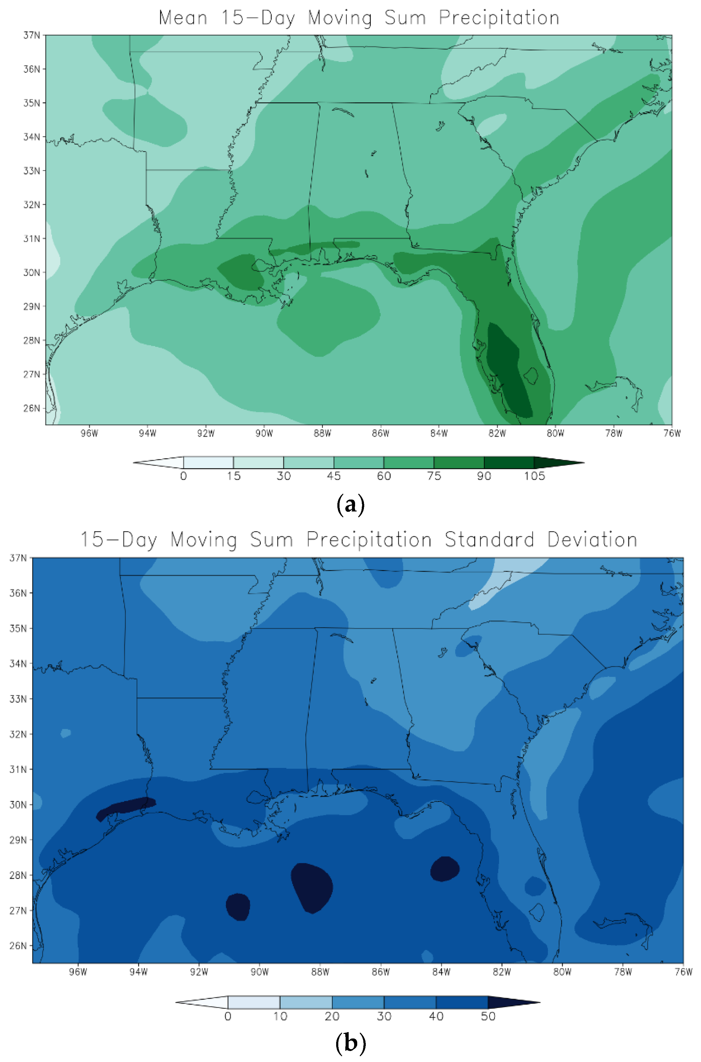
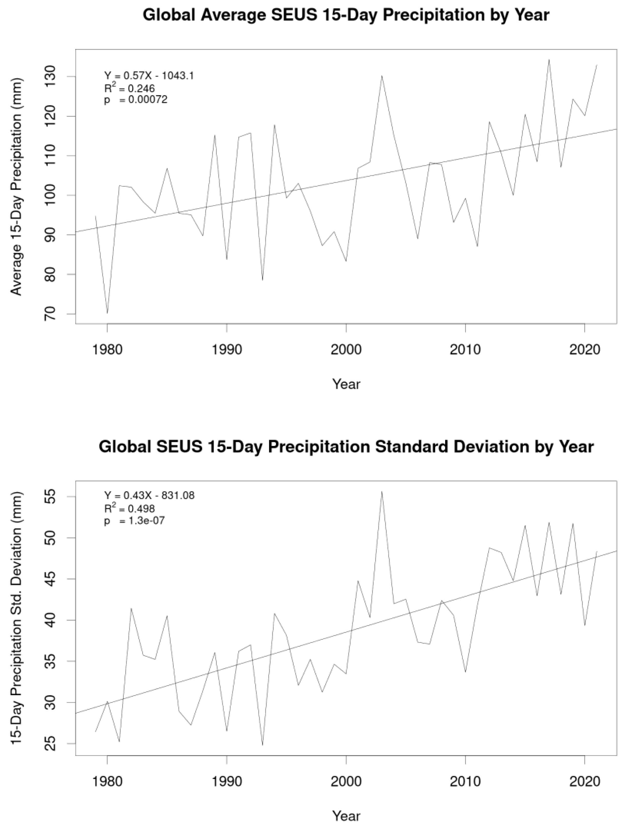
Spatially, the selected study domain comprised 3341 NARR grid points over the SEUS. Figure 2a shows the mean 15-day moving sum warm season SEUS precipitation accumulation for the full period over the study domain. The standard deviation is provided as well as a measure of spread about the mean (Figure 2b). The mean pattern (Figure 2a) shows the well-established [2] maximum of precipitation along the Gulf and Atlantic coasts. As expected, the increased variability associated with the less reliable satellite-derived precipitation estimates over the Gulf of Mexico and Atlantic was also evident in the standard deviation fields (Figure 2b). Related to the spatial means, we also computed the annual means for each spatial field, as well as their standard deviations (Figure 3).
This analysis revealed a statistically significant positive trend in both the mean (p = 0.0007) and standard deviation (p = 1.3 × 10⁻⁷), suggesting that, for the entirety of the domain, 15-day aggregated precipitation has become both more plentiful and more variable over the 40-year study period.
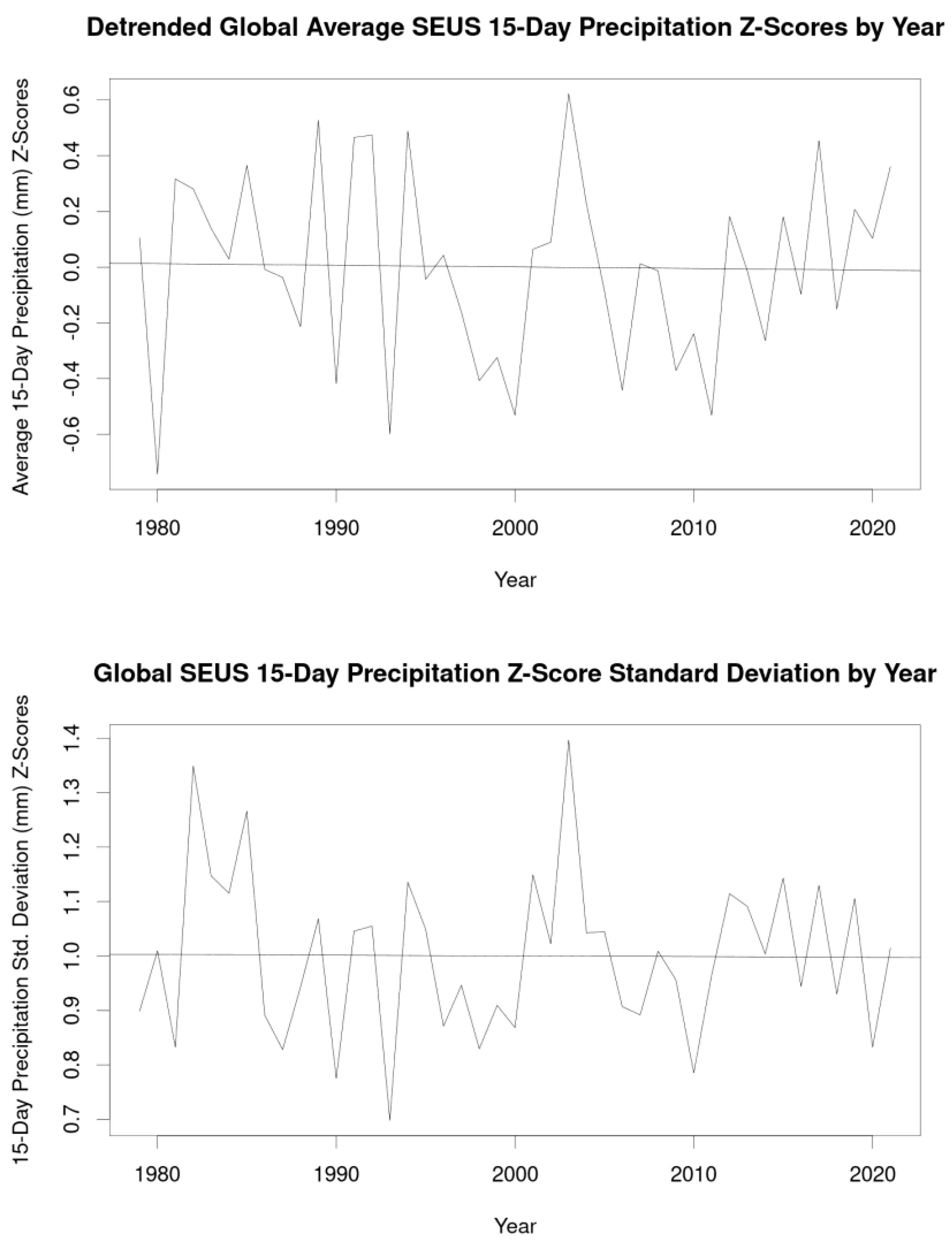
When performing cluster analysis on data with a strong temporal trend (Figure 3), it is important to detrend the fields prior to the analysis to ensure the primary clustering is not simply detecting the temporal shift. Thus, we standardized these fields by formulating a linear fit (equations provided in Figure 3) for the annual means and standard deviations. We computed the modeled annual mean and standard deviation for each year and computed z-scores at each grid point using those detrended annual mean and standard deviations. The resulting time series (Figure 4) showed no upward trend, as well as nonsignificant slopes (p = 0.89 for the means, p = 0.94 for the standard deviations), which ensured the cluster analysis would be standardized relative to individual precipitation years, not based on the strong upward trend portrayed in Figure 3. These detrended annual z-scores were used as input into the cluster analysis methods described below.

2.2. Cluster Analysis Methodology

As shown above, numerous studies [8,22,23] have employed cluster analysis when isolating synoptic-scale structures associated with SEUS precipitation patterns. The two most common types of cluster analysis methods (k-means and hierarchical) utilize statistical distance (often Euclidean) to quantify the similarity among points within a dataset [20]. Hierarchical methods group clusters with the smallest Euclidean distance, based on a given cluster linkage method, while k-means attempts to minimize intracluster separation while maximizing intercluster separation through convergence of the algorithm on a set of optimal cluster centers. An important limitation of these approaches is an underlying assumption that the data are linearly separable, which is not always the case.
Recent studies have shown improved clustering by preprocessing the analysis using principal component analysis [PCA-20], which decomposes the database into dominant variability modes. This method has shown some benefit, but as PCA uses a linearly based similarity matrix (traditionally the correlation or covariance matrix), this approach still has an inherent linear assumption. More recent developments by [19] suggested an alternative similarity matrix could be employed to characterize nonlinear variability. This alternative matrix, the kernel matrix K from support vector machines [27], retains the original characteristics of a correlation/covariance matrix (positive definite, symmetric, and nonsingular) while representing the data in a nonlinear Hilbert space where previously unseen nonlinear separability can be discovered and quantified. This approach, known as kernel PCA (KPCA), was used in our study to assess the presence of any such nonlinear relationships within the SEUS precipitation anomaly fields.
The KPCA mathematical approach [19,21] is almost identical to linear PCA (except for the computation and centering of the similarity matrix) in that it employs eigenanalysis on a similarity matrix (here K) to obtain basis vectors that describe the data variability. The eigenanalysis equation used in KPCA (Equation (1)) is calculated by:
K c e n t e r α i = λ i α i
where αi and λi are eigenvalues and eigenvectors of Kcenter, and Kcenter is a centered kernel matrix computed from Equation (2):
K c e n t e r = K 2 1 1 n K + 1 1 n K 1 1 n
where 1 1 n is a matrix whose elements are all 1 n where n is the number of columns of K (in our study, the 43 years of data). The centering step is required as K does not guarantee a centered similarity matrix, a requirement of eigenanalysis. While numerous matrices can serve as K, there are two functions that are used most frequently when computing K, a polynomial kernel (Equation (3)) or a radial basis function (RBF) kernel (Equation (4)):
K ( x , y ) = ( x y + 1 ) d
K ( x , y ) = exp ( 1 2 σ 2 | | x y | | 2 ) .
In most applications of KPCA, the vector y is simply y = x T , as this approach constructs a symmetric K. For the polynomial kernel, the variable d represents the degree of the polynomial, while σ represents the spread of the radial basis function kernel. These values should be tuned to yield different solutions for K, with the goal of finding the global minimum in cluster cohesion (intracluster separation) with a maximum in intercluster separation. Note that traditional PCA will yield similar results to polynomial kernel KPCA when d = 1 (a linear kernel).
An important limitation of KPCA is its direct interpretability. In many rotated PCA studies [28,29], it is possible to interpret the resulting loading matrix (eigenvectors scaled by the square root of their eigenvalue) directly, since the transformation was linear. With KPCA, the use of an unknown kernel map function φ(x) confounds the ability to back-transform the data to the original data space. Instead, the dot product of φ(x) with itself or another kernel map function yields the matrix K by the kernel trick [27], which does not require a priori knowledge of φ(x). While this limits direct interpretability, the resulting KPC loadings can be used as an input into a traditional cluster analysis method (in our study we used k-means), which potentially provides updated clusters based on the nonlinear relationships characterized by the kernel transformation.
Selecting the optimal number of loadings to retain, which is a recurring problem with all PCA approaches [28,29], becomes more challenging with KPCA for reasons outlined above. Additionally, the k-means approach has an inherent limitation that the number of clusters must be known before the method can be used. For our study, we tested between three and eight clusters. These values were somewhat arbitrary, though more than eight clusters decreased the quality of the analysis by resulting in multiple single-member clusters (not shown), while two clusters yielded results very similar to the SEUS mean. We also tested retaining between two to 42 KPC loadings (as the 43rd eigenvalue always has a magnitude of zero), as well as multiple values for d (all integers spanning 1 to 4) and σ (all integers from 10 to 200) for the polynomial and RBF kernels, respectively. In total, 47,970 permutations of retained clusters, loadings kept, and kernel configurations were tested to search for an optimal maximum that minimized cluster cohesion and maximized inter-cluster separation. This extensive testing increased the likelihood that a global maximum in cluster analysis performance could be found. As a baseline, we also formulated a k-means analysis directly on the anomaly fields to ascertain what benefit, if any, the KPCA preprocessing offered to the analysis, and thereby determine the extent of nonlinear relationships within the precipitation fields.
Quantifying the quality of the clustering, which was critical for identifying the optimal configuration from among the possible tested analysis methods, was done uing a combined method implementing the silhouette coefficient [30] and the average correlation between the cluster members and their composite mean. A metric derived from [31] was used to quantify the global silhouette coefficient performance from each permutation using Equation (5):
S * = ( 1 m s N ) ( S ¯ )  
where N is the total number of samples, ms is the number of misclassified clusters (based on negative S values), and S ¯ is the average of all silhouettes for the given cluster configuration. Some kernel configurations (mostly the polynomial kernels) yielded multiple clusters that comprised only 1–2 precipitation years, with one cluster retaining the remaining 40 years. These configurations yielded the highest values for S * owing to the proximity of a single case with its composite mean (e.g., the mean of a cluster of one is just that case, so its distance from the mean is zero). These results were undesirable, as the resulting analysis yielded one large cluster composite that closely resembled the global mean for all years while remaining clusters comprised individual cases with inflated S* values. We minimized this issue by using a weighted mean for S*, computed using Equation (6) as:
S ¯ = i = 1 n N i N ( S ¯ i )
where i represents a given cluster number from the given analysis. This approach placed higher emphasis on clusters with larger numbers of members, which reduced the inflation of S * with clusters that contained only 1–2 events.
Once the weighted S* value was computed for each permutation, they were compared against a baseline S* from the cluster analysis that did not include any KPCA preprocessing. All KPCA-preprocessed results, if any, whose S* value exceeded the baseline value for the given number of clusters were retained for further analysis.
Once the subset of KPCA preprocessed cluster results was obtained, the composite mean of each cluster’s precipitation anomalies was computed. These composite means were correlated against the individual cluster’s constituent years, and the average of these cluster correlations was computed as a measure of cluster match to its constituent cases. The configuration that yielded both an S* exceeding the baseline and the highest average correlation among clusters was retained as the optimal configuration. Note that this was calculated for each number of retained clusters separately, since the average correlation between clusters and their members naturally increases as the number of clusters increases (owing to smaller cluster memberships with larger numbers of clusters—see Table 1 and Table 2 below). This trend was not noticeable with S*. Outcomes from these analyses, as well as the composite fields that resulted from the optimal clustering method, are presented in Section 3.

3. Results

3.1. Cluster Analysis Overall Results

As mentioned above, 47,970 possible loading–kernel–cluster combinations were tested to search for the clustering methodology that maximized S * . The highest S * (0.105) resulted from retaining three clusters using a linear kernel with KPCA preprocessing. However, the benefits of KPCA were minimal, as seen in the results for the baseline (Table 1) and KPCA-preprocessed (Table 2) cluster analysis. Note that S * values considerably higher than the best performing cluster analysis method were observed when employing polynomial kernels (discussed above) but given how the cases were distributed among the clusters (not shown), these results were discarded.
The optimal KPCA-preprocessed results differed from the baseline cluster analysis by moving one year, 2005, from cluster 2 to cluster 1, which led to a minimal increase of S* (in the 4th decimal place, not shown). This result was consistent among all cluster configurations apart from retaining six clusters, in which no KPCA preprocessed result outperformed regular k-means analysis. For most configurations tested (except three clusters), the best kernel for KPCA was consistently the radial basis function (RBF) with σ values of similar magnitude as the NARR grid spacing (32-km). Overall, the three-cluster solution using KPCA preprocessing with a linear kernel was used as the primary analysis method for constructing the precipitation composites.
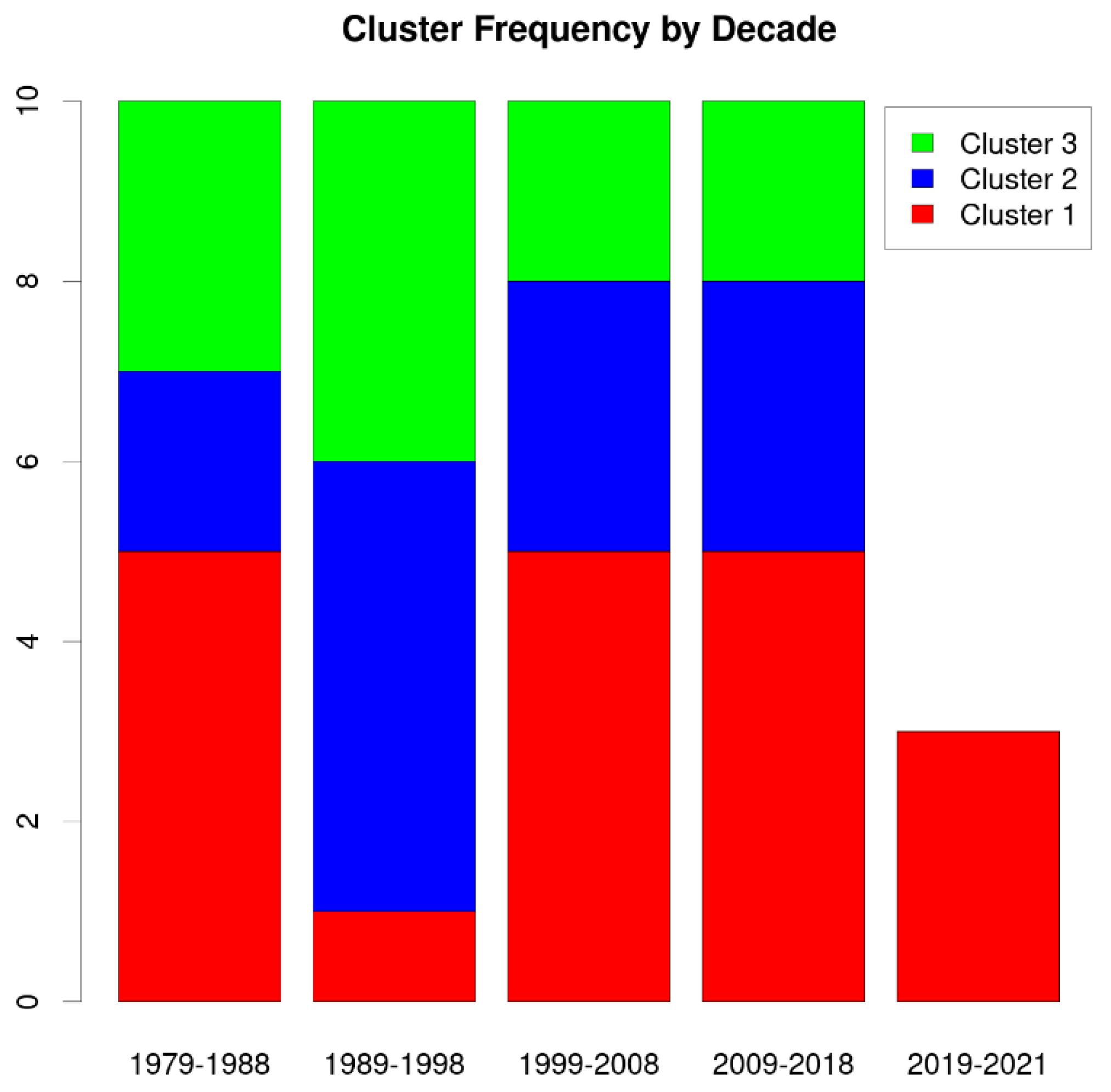
The selected optimal configurations resulted in groups of size 19, 13, and 11 for clusters 1–3 (note that cluster number is arbitrary so for this study they are sorted by decreasing size). The resulting clusters showed interesting temporal trends (Figure 5). First, other than the notable drop in frequency during the 1989–1998 period, the cluster 1 occurrence rate remained relatively consistent over the study period, suggesting it could be related to a mean pattern. Notably, the last three study years were also all entirely grouped into cluster 1. Cluster 2′s frequency shows a different yet consistent trend, as its frequency was highest during the 1989–1998 period and held steady for the last 20 years of the study period. The results suggest that a possible decadal trend in the precipitation arrangement in the SEUS is plausible, but more study years are needed to ensure this is the case. Cluster 3′s results maintained a similar occurrence rate for all four decades presented in Figure 5 but has become slightly more infrequent in recent decades.
The silhouette coefficients for the optimal configuration used in this study were telling as well. The configuration yielded seven negative (misclustered) S values, six of which were with cluster 1 (and were proximal to cluster 2). Cluster 1′s average S among its members was 0.037, which was the lowest of all clusters (a result of the abundant negative S values). Cluster 2′s results showed the highest overall average S (0.222), while cluster 3 had a value near the global S* for the entire analysis (0.086). These results are important for several reasons. First, they suggest there may be additional clusters to be gained from cluster 1, which we deemed the mean cluster (see below). Second, the distinctiveness of cluster 2′s silhouette values show it is the best separated of all clusters and its results are most likely to match its respective cases. Finally, the cluster 3 average S values falling near the global S* suggests cluster 3 is showing a pattern that is consistently distributed in time among the clusters, which is seen in Figure 5 above.
In addition to quantifying the cluster quality via the silhouette coefficient, we also computed the average correlation between the constituent members and each cluster’s composite mean precipitation map. These correlations scaled as a function of sample size, with cluster 1′s average correlation at 0.830, cluster 2 at 0.706, and cluster 3 at 0.792. Cluster 1 resembles the mean pattern (see below), and this elevated correlation coupled with the largest sample size suggests the mean pattern is frequently in place in the SEUS and has been consistent outside of the 1989–1998 decade. Likewise, the cluster 2 results (the dry cluster, see below) have a much lower correlation, suggesting there may be multiple configurations of “dry” SEUS conditions that should be explored in future work. Cluster 3′s intermediate correlation suggests the wet pattern (see below) is more consistent than the dry pattern but there is still likely greater variability than with the mean.
Overall, the global S* values were quite low relative to other clustering studies that used a similar metric [18,21,29,31]. This relatively low performance demonstrates the lack of separability in these precipitation fields, suggesting precipitation patterns over the SEUS likely deviate only slightly from the mean in most instances.

3.2. Cluster Map Results

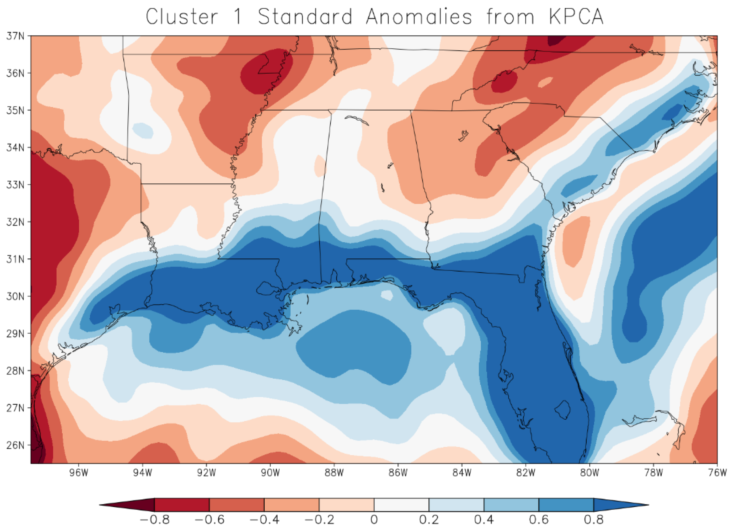
The presented cluster analysis results are provided by arbitrary cluster numbers, so the clusters are sorted by decreasing sample size (same as discussed in Section 3.1). Cluster 1′s composite map (Figure 6) correlated most strongly with the mean of all years (r = 0.963). Its local precipitation maximum along the Gulf and Atlantic Coasts was also evident in the mean field (Figure 2), and the areas of low precipitation farther inland in the mean field were portrayed as well. This cluster had the highest membership count (N = 19), suggesting that the mean pattern is overall most prevalent. The coastal maxima in precipitation seen in these fields are consistent with daily sea breeze precipitation as well as tropical cyclone landfalls (discussed further below). Additionally, work in [4,32] showed the impacts of agriculture in reducing precipitation amount in the Mississippi Delta region and along the Mississippi River in Arkansas and Tennessee. The mean field reflected this lack of precipitation relative to the background mean state, suggesting that this pattern is not only present, but it is the most frequently observed precipitation state for this part of the study region. The dry regions along the Appalachians are associated with similar impacts and seen in [33] as well, as their study noted a localized precipitation magnitude ridge along the Georgia–South Carolina–North Carolina border, slightly west of the minimum over the central Carolinas and Virginia.
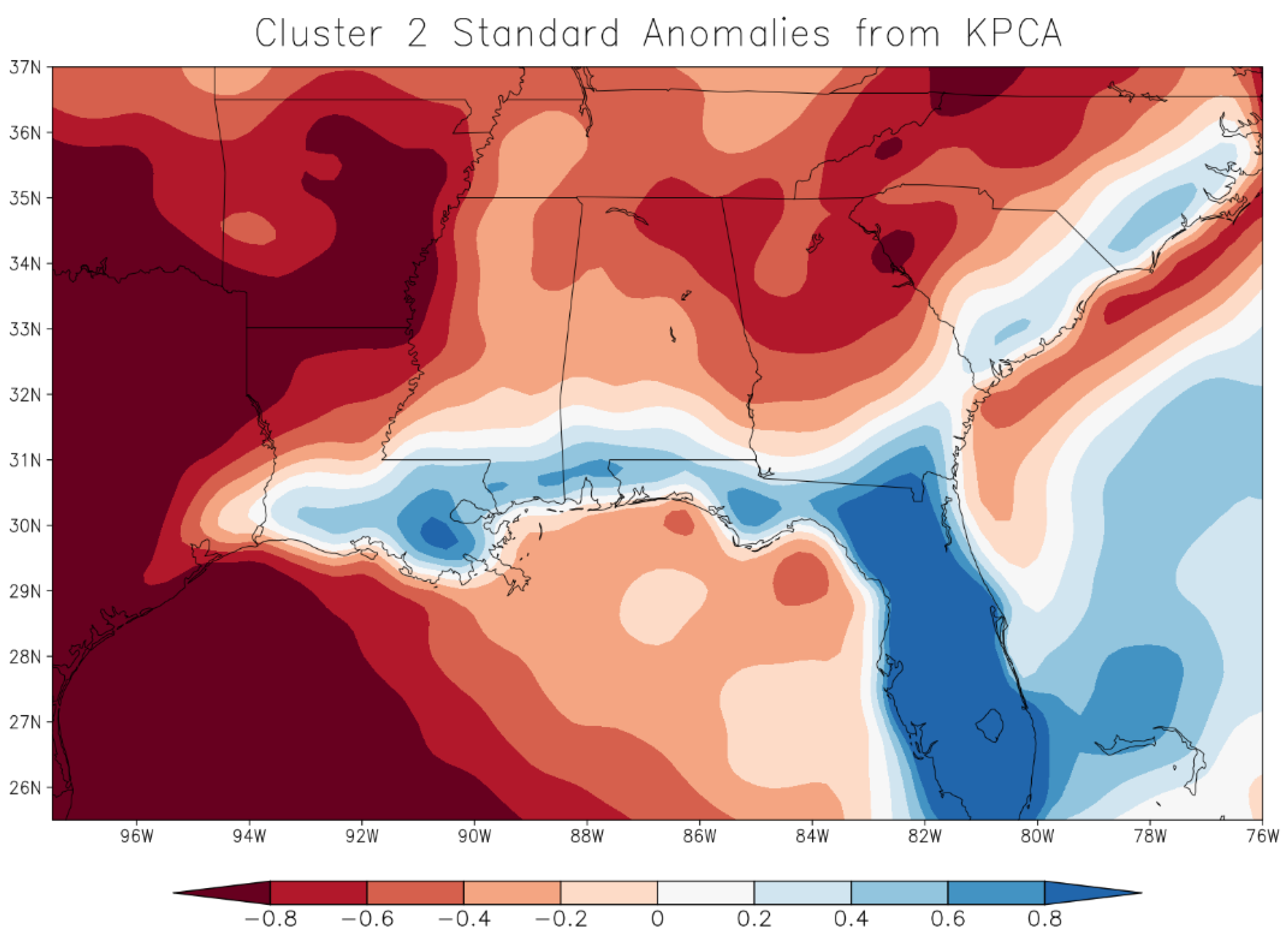
In Cluster 2 (Figure 7), the general shape of the pattern matches the mean pattern, though its correlation with the mean is the lowest of the three clusters (r = 0.903). Instead, the largest differences result from magnitude shifts in the pattern, as precipitation magnitudes are consistently lower across the entire study region. Notably, the dry regions in the western SEUS states have expanded much farther eastward in this cluster, now encompassing central and eastern states as well. The two separate dry regions in cluster 1 seemingly have merged into a larger dry region. Additionally, the coastal precipitation, while still elevated relative to the remaining SEUS regions, showed considerable shrinking of the maximum. This suggests that disregarding the precipitation associated with the sea breeze circulation along the coast, precipitation patterns are drier across the entire study domain. These results are consistent with their cluster membership, as the highly impactful droughts of 1988 [34] and 1993 [35], among others, were members of cluster 2 and highly correlated with its spatial pattern (r = 0.863 and r = 0.765, respectively). The results shown in Figure 5 suggest each decade is associated with roughly 30% of years constituting drought conditions, though in recent years cluster 2′s membership has dwindled as its last member year was 2014.
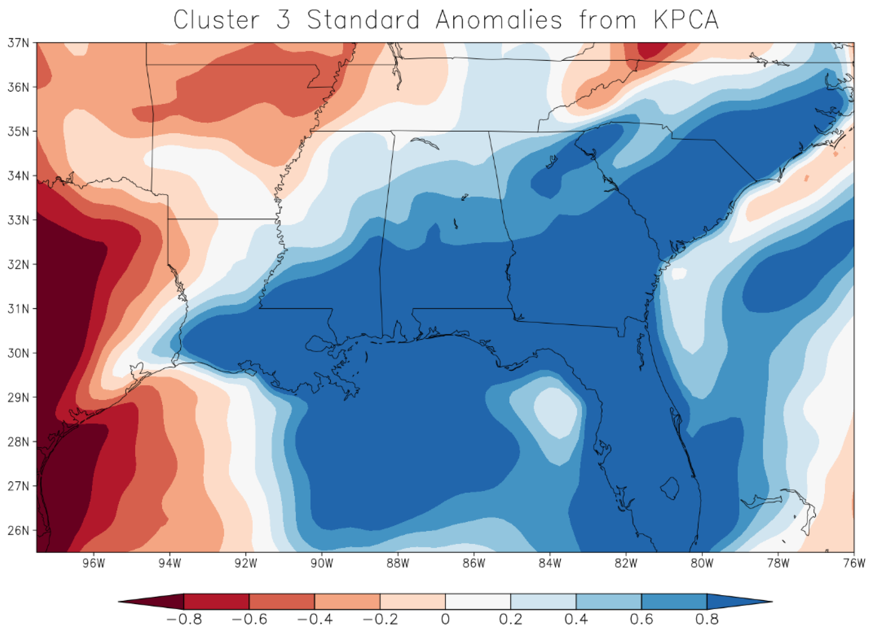
Cluster 3′s results (Figure 8) contrasted most prominently with cluster 2, as it showed abundant above-average precipitation across most of the SEUS study region. It matches the global mean pattern slightly better than cluster 2 (r = 0.930) but not as well as cluster 1. The pattern showed an apparent spreading of the precipitation maximum along the Gulf Coast to extend into central regions of the Gulf and Atlantic Coast states. The influence of the drier air in the Desert Southwest is still evident in the western portions of this cluster, but the region is confined much farther west as was seen in cluster 1. New key features emerged in this cluster as well. First, the small precipitation ridge in northeastern Georgia and along the western North Carolina/South Carolina border discussed in [33] was more pronounced in this pattern than in cluster 1. Likewise, the relative dryness in the Mississippi Delta region was missing in this cluster, despite lower precipitation values remaining in Arkansas (a consequence of its proximity to the Great Plains and the influence of the drier conditions in the southwest).
Overall, the clusters showed strong similarities in terms of the dominant spatial features. All clusters showed the driest conditions in the western portions of the SEUS study domain, which resulted from the influence of more abundant drier conditions from the desert southwest and its continental tropical air mass. All patterns also showed the abundant coastal precipitation observed in the mean field, as well as relatively reduced precipitation in the southern Appalachians (with the notable exception of the small precipitation ridge in the western Carolinas and northeastern Georgia that was most apparent in cluster 3). The similarities in these clusters were apparent in their correlations, as clusters 1 and 2 correlated at 0.837, clusters 1 and 3 at 0.852, and 2 and 3 at 0.835. Clearly, the cluster analysis was detecting differences in magnitudes, not pattern, in establishing the dominant precipitation patterns for the SEUS.

4. Discussion

To quantify the physical nature of the environment characterizing the different SEUS warm-season precipitation clusters, simple composite average maps of base-state meteorological fields were constructed for each cluster using fields from the NARR. Expectedly, these fields characterized a nearly barotropic environment for the full SEUS, with minimal kinematic influences on precipitation as upper-level winds did not exceed 15 m/s for any upper-level composite (not shown). Similarly, low-level kinematics were largely barotropic, as seen by the minimal height gradient observed in Figure 9 for the 850 mb composite fields. Moisture was largely the same for each composite field as well, but the warmer conditions associated with the dry composite (cluster 2—Figure 9b) were clear in the western third of the domain as the hot dry air from the desert southwest had advanced farther eastward in that composite. All fields, as expected via the traditional general circulation model, are dominated by the subtropical high, further reinforcing the thermodynamic nature of the precipitation processes that dominate SEUS warm season precipitation.
In addition to the composite analysis, we investigated how each pattern related to important climate drivers for SEUS warm season precipitation, namely the El-Niño–southern oscillation [36] and tropical cyclone activity [10,11]. To quantify the ENSO phase associated with each cluster, we used Oceanic Niño Index (ONI [37]) monthly data for the warm season months for each year, using their mean to establish a single ONI for each annual warm season (Figure 10 top panel). Instances where the ONI fell below −0.5 or above 0.5 were indicated as a La Niña or El Niño event, respectively [37].
For our full study period, the ONI data showed 7 warm season SEUS La Niña patterns, 6 El Niño patterns, and 30 neutral phases (Figure 10, top panel). In cluster 1, 73.7% of its member years were neutral ENSO phases, while 15.8% were El Niño and 10.5% La Niña. However, cluster 1′s results did include two very strong El Niño events (1987 and 2015) as well as one moderately strong La Niña in 2010. The prevalence of neutral patterns and balance between El Niño and La Niña did not show a favorability of cluster 1 towards a given phase of ENSO, which reinforces the earlier conclusion that this field is most like a mean pattern for precipitation.
This result contrasts starkly with the results for cluster 2, which had numerous members in the La Niña phase (30.8%) with only 61.5% neutral and 7.7% in the El Niño phase. This second pattern, which is a strongly dry pattern, is consistent with the literature regarding ENSO phase and SEUS precipitation, namely that La Niña patterns are associated with drier conditions [36]. Cluster 3′s results showed the highest prevalence of El Niño events (18.1%) relative to its cluster size, as well as a similar prevalence of neutral ENSO phases (72.7%) and the lowest La Niña percentage (9.1%). However, the differences in these ratios between clusters 1 and 3 are not dramatic, which suggests that an El Niño could result in a structure more in line with either cluster 1 or 3. As the El Niño phase is generally associated with more abundant SEUS precipitation, this result is consistent with the patterns portrayed by the cluster analysis.
Previous studies ([10,11] and others) have shown the importance of landfalling tropical cyclones (Figure 10 bottom panel) on above-average SEUS precipitation. To establish significant differences among the clusters in terms of tropical cyclone landfalls, we computed 95% bootstrap confidence intervals [38] for each cluster’s landfall count (Table 3). These results revealed a statistically significant decrease in tropical cyclone landfalls for cluster 2 when compared to both clusters 1 and 3. This result reinforces the results in [10,11] that suggest tropical cyclone landfalls are important precipitation moderators during the SEUS warm season. Notably, no significant differences exist between clusters 1 and 3, suggesting abundant tropical cyclone landfalls are having less of an effect on high precipitation SEUS warm season patterns.
The year 2005 was isolated as a unique year by the cluster analysis, as the only difference between the KPCA and traditional analyses was the placement of 2005 in cluster 1 (with KPCA) versus cluster 2 (without KPCA). The precipitation anomaly field for 2005 (Figure 11) shows a pattern with highly abundant precipitation along the coast and into Georgia and South Carolina, more in line with a pattern expected to fall in cluster 3. However, notably dry conditions were present across the Mississippi River Valley, which was more aligned with cluster 2′s pattern. Hence, the placement in cluster 1 (the near-mean pattern) was deemed more appropriate for 2005. The 2005 hurricane season was an historic event, with six strong landfalling tropical cyclones (including hurricanes Katrina, Rita, and Wilma) that all traversed the heavy precipitation region in Figure 11. It is likely that without those strong storms, 2005 would have been clustered with cluster 2, based on its relatively low precipitation elsewhere, showing how a single year had a dramatic influence on the overall SEUS precipitation climatology. This result shows KPCA’s ability to detect anomalous features within the dataset and cluster those features more appropriately, demonstrated by the boost in S* and the overall blend of clusters 2 and 3 present in the 2005 season. We expect that as the sample size of precipitation years increases, this sensitivity of the cluster analysis to individual outlier years will be reduced.

5. Conclusions

SEUS warm season precipitation is a critical resource for regional agricultural productivity and hydrologic processes, making it a key factor in social and economic sustainability. However, as warm season rainfall is driven primarily by thermodynamic (convective) processes that have inherently low predictability, prior knowledge of abundant and limited precipitation regions via climatological analysis can have value when identifying water resource patterns and sensitive areas. Numerous previous studies [2,3,4,5,6,7,8,9,10,11,12,14,15,22,23,24] have investigated different aspects of SEUS precipitation, either by region (such as the Appalachian or coastal areas) or by meteorological mechanisms responsible for the precipitation. However, these studies were inherently limited to monthly time scales and utilized primarily linear techniques when identifying dominant precipitation patterns. This limitation could result in the loss of nonlinear variability information that may be important in SEUS precipitation climatology. Hence, the objective of our study was to develop an updated warm season SEUS precipitation climatology based on 15-day moving sums and employ a nonlinear cluster analysis method via kernel PCA to define temporal clusters.
When applying KPCA-preprocessing to the 15-day moving sum SEUS precipitation fields, we found that three primary clusters were consistently prevalent within those fields. All three clusters (Figure 6, Figure 7 and Figure 8) strongly resembled the mean field (Figure 2a) in terms of the spatial shape of the precipitation (r > 0.9), but magnitudes of each cluster were dramatically different. Cluster 1 (N = 19) showed a pattern that most strongly resembled the mean pattern in terms of its shape, and the precipitation anomaly magnitudes were intermediate between the other two clusters, suggesting cluster 1 was the mean precipitation pattern. This pattern, much like the global mean in Figure 2a, was associated with abundant precipitation along the Gulf and Atlantic Coasts that was primarily associated with sea breeze effects and tropical cyclone landfalls, as well as a relative lack of precipitation over the western portion of the domain and southern Appalachians. We also identified a small regional precipitation ridge encompassing northeastern Georgia and the western North Carolina/South Carolina border that was consistent with precipitation climatology work seen in [33]. Cluster 2′s pattern (N = 13) showed considerably drier conditions throughout the study domain, while cluster 3′s pattern (N = 11) showed the wettest conditions of the three clusters. All clusters correlated strongly with the mean pattern, with cluster 1 showing the strongest relationship (0.963).
Expectedly, the synoptic composite fields associated with each cluster revealed a strongly barotropic environment with minimal thermal gradients that was dominated by the subtropical high. When comparing the resulting composites with climate-scale precipitation drivers, we noted that cluster 2 was strongly associated with La Niña conditions, while clusters 1 and 3 showed a similar percentage of both neutral and El Niño phases. Likewise, cluster 2 showed a statistically significantly lower tropical cyclone landfall frequency, suggesting that the drier conditions from the La Niña coupled with reduced landfalling tropical cyclones led to the dearth of precipitation. Notably, KPCA preprocessing made only a marginal improvement in the cluster metric S* (roughly 2%) as it suggested shifting the 2005 annual pattern from cluster 2 (the dry cluster) to cluster 1 (the mean cluster). As 2005 was associated with notably high tropical cyclone frequency but had drier conditions throughout the rest of the SEUS, the difficulty in clustering 2005 was not surprising but demonstrated the added value of the KPCA.
There were several limitations to this work. First, the NARR precipitation data, while continuous in time and space, are still based on a model-derived reanalysis product that has some inherent limitations (especially over water). The somewhat arbitrary selection of a 15-day moving sum could have affected the results as well, though we tested 31- and 45-day centered moving sums (not shown) and results were similar. It is possible the KPCA methodology did not identify the local maximum in cluster analysis performance, as several configurations yielded notably high S* values but retained a mean field with clusters of 1–2 members as the remaining cases. Additional cluster analysis methods should be explored in future work.
Overall, we have reinforced the work of several studies that considered SEUS precipitation climatology and have found that those results hold up even when tested with a nonlinear cluster analysis method. These results revealed localized challenges in water resources, most notably the risk for flooding in southern Appalachian areas and along the coastlines, as well as those areas which may be more sensitive to drought in the western SEUS region and along the Mississippi River. This climatology can help inform future studies investigating water resources available from warm season SEUS precipitation.

Author Contributions

Conceptualization, A.M. and J.D.; methodology, A.M.; software, A.M.; validation, A.M. and J.D.; formal analysis, A.M. and J.D.; data curation, A.M.; writing—original draft preparation, A.M.; writing—review and editing, A.M. and J.D.; visualization, A.M.; project administration, A.M.; funding acquisition, J.D. All authors have read and agreed to the published version of the manuscript.

Funding

This research was funded by the National Oceanic and Atmospheric Administration award number NA19OAR4590411.

Institutional Review Board Statement

Not applicable.

Informed Consent Statement

Not applicable.

Data Availability Statement

Data used in this study are freely available from the National Oceanic and Atmospheric Administration’s National Center for Environmental Information.

Conflicts of Interest

The authors declare no conflict of interest.

References

  1. United States Department of Agriculture. Quick Statistics. National Agricultural Statistics Service. 2021. Available online: https://quickstats.nass.usda.gov (accessed on 31 October 2022).
  2. Qian, J.; Viner, B.; Noble, S.; Werth, D. Precipitation characteristics of warm season weather types in the Southeastern United States of America. Atmosphere 2021, 12, 1001. [Google Scholar] [CrossRef]
  3. Lu, C.; Zhang, J.; Tian, H.; Crumpton, W.; Helmers, M.; Cai, W.; Hopkinson, C.; Lohrenz, S. Increased extreme precipitation challenges load management to the Gulf of Mexico. Nat. Commun. Earth Environ. 2020, 1, 1–10. [Google Scholar] [CrossRef]
  4. Dyer, J.; Mercer, A. Identification of recharge zones in the Lower Mississippi River alluvial aquifer using high-resolution precipitation estimates. J. Hydrol. 2015, 531, 360–369. [Google Scholar] [CrossRef]
  5. Tashie, A.; Mirus, B.; Pavelsky, T. Identifying long-term empirical relationships between storm characteristics and episodic groundwater recharge. Water Resour. Res. 2015, 52, 21–35. [Google Scholar] [CrossRef] [Green Version]
  6. Moore, B.; Mahoney, K.; Sukovich, E.; Cifelli, R.; Hamill, T. Climatology and environmental characteristics of extreme precipitation events in the Southeastern United States. Mon. Weather Rev. 2015, 143, 718–741. [Google Scholar] [CrossRef]
  7. Keim, B. Spatial, synoptic, and seasonal patterns of rainfall in the southeastern United States. Phys. Geogr. 1996, 17, 313–328. [Google Scholar] [CrossRef]
  8. Konrad, C. Synoptic-scale features associated with warm season heavy rainfall over the interior Southeastern United States. Weather Forecast. 1997, 12, 557–571. [Google Scholar] [CrossRef]
  9. Shepherd, J.; Grundstein, A.; Mote, T. Quantifying the contribution of tropical cyclones to extreme rainfall along the coastal southeastern United States. Geophys. Res. Lett. 2007, 34, L23810. [Google Scholar] [CrossRef]
  10. Knight, D.; Davis, R. Contribution of tropical cyclones to extreme rainfall events in the southeastern United States. J. Geophys. Res. 2009, 114, D23102. [Google Scholar] [CrossRef] [Green Version]
  11. Konrad, C.; Perry, L. Relationships between tropical cyclones and heavy rainfall in the Carolina region of the USA. Int. J. Climatol. 2010, 30, 522–534. [Google Scholar] [CrossRef]
  12. Seager, R.; Tzanova, A.; Nakamura, J. Drought in the southeastern United States: Causes, variability over the last millennium, and the potential for future hydroclimate change. J. Climate 2009, 22, 5021–5045. [Google Scholar] [CrossRef] [Green Version]
  13. Seager, R.; Ting, M.; Davis, M.; Cane, M.; Naik, N.; Nakamura, J.; Li, C.; Cook, E.; Stahle, D. Mexican drought: An observational modeling and tree ring study of variability and climate change. Atmósphera 2009, 22, 1–31. [Google Scholar]
  14. Schubert, S.; Chang, Y.; DeAngelis, A.; Wang, H.; Koster, R. On the development and demise of the Fall 2019 Southeast U.S. flash drought: Links to an extreme positive IOD. J. Climate 2021, 34, 1701–1723. [Google Scholar] [CrossRef]
  15. Dyer, J.; Mercer, A.; Raczynski, K. Quantifying spatial patterns of hydrologic drought over the Southeast US using retrospective National Water Model simulations. Water 2022, 14, 1525. [Google Scholar] [CrossRef]
  16. National Oceanic and Atmospheric Administration Office of Weather Prediction (OWP). The National Water Model. 2022. Available online: https://water.noaa.gov/about/nwm (accessed on 31 October 2022).
  17. Hsieh, W. Machine Learning Methods in the Environmental Sciences; Cambridge University Press: Cambridge, UK, 2009; pp. 16–18. [Google Scholar]
  18. Mercer, A.; Leslie, L.; Richman, M. Identification of severe weather outbreaks using kernel principal component analysis. Proc. Comp. Sci. 2011, 6, 231–236. [Google Scholar] [CrossRef] [Green Version]
  19. Schölkopf, B.; Smola, A.; Müller, K. Kernel principal component analysis. In International Conference on Artificial Neural Networks; Springer: Berlin/Heidelberg, Germany, 1997; pp. 583–588. [Google Scholar]
  20. Wilks, D. Statistical Methods in the Atmospheric Sciences; Elsevier Press: Amsterdam, The Netherlands, 2019; pp. 721–738. [Google Scholar]
  21. Mercer, A.; Grimes, A.; Wood, K. Application of unsupervised learning techniques to identify Atlantic tropical cyclone rapid intensification environments. J. Appl. Meteorol. Clim. 2021, 60, 119–138. [Google Scholar] [CrossRef]
  22. Sugg, J.; Konrad, C. Defining hydroclimatic regions using daily rainfall characteristics in the southern Appalachian Mountains. Int. J. Digit. Earth 2019, 1–18. [Google Scholar] [CrossRef]
  23. Sugg, J.; Konrad, C. Relating warm season hydroclimatic variability in the Southern Appalachians to synoptic weather patterns using self-organizing maps. Clim. Res. 2017, 74, 145–160. [Google Scholar] [CrossRef]
  24. Dyer, J. Basin-scale precipitation analysis for southeast U.S. watersheds using high-resolution radar precipitation estimates. Phys. Geogr. 2008, 29, 320–340. [Google Scholar] [CrossRef]
  25. Mesinger, F.; DiMego, G.; Kalnay, E.; Mitchell, K.; Shafran, P.; Ebisuzaki, W.; Jović, D.; Woolen, J.; Rogers, E.; Berbery, E.; et al. North American Regional Reanalysis. Bull. Am. Meteorol. Soc. 2006, 87, 343–360. [Google Scholar] [CrossRef] [Green Version]
  26. Kalnay, E.; Kanamitsu, M.; Kistler, R.; Collins, W.; Deaven, D.; Gandin, L.; Iredell, M.; Saha, S.; White, G.; Woollen, J.; et al. The NCEP/NCAR 40-year reanalysis project. Bull. Am. Meteorol. Soc. 1996, 77, 437–472. [Google Scholar] [CrossRef]
  27. Cristianini, N.; Shawe-Taylor, J. An Introduction to Support Vector Machines; Cambridge University Press: Cambridge, UK, 2000; pp. 1–182. [Google Scholar]
  28. Barnston, A.G.; Livezey, R.E. Classification, seasonality and persistence of low-frequency atmospheric circulation patterns. Mon. Weather Rev. 1987, 115, 1083–1126. [Google Scholar] [CrossRef]
  29. Mercer, A.; Richman, M. Assessing atmospheric variability using kernel principal component analysis. Proc. Comp. Sci. 2012, 7, 288–293. [Google Scholar] [CrossRef] [Green Version]
  30. Rousseeuw, P. Silhouettes, a graphical aid for the interpretation and validation of cluster analysis. J. Comp. Appl. Math. 1987, 20, 53–65. [Google Scholar] [CrossRef] [Green Version]
  31. Mercer, A. Dominant United States cold-season near surface temperature anomaly patterns derived from kernel principal component analysis. Int. J. Climatol. 2021, 41, 2383–2396. [Google Scholar] [CrossRef]
  32. Dyer, J. Evaluation of Surface and Radar-Estimated Precipitation Data Sources Over the Lower Mississippi River Alluvial Plain. Phys. Geogr. 2009, 30, 430–452. [Google Scholar] [CrossRef]
  33. Gaffin, D.; Hotz, D. A precipitation and flood climatology with synoptic features of heavy rainfall across the southern Appalachian mountains. Natl. Weather Dig. 2000, 24, 3–15. [Google Scholar]
  34. Chagnon, S. The 1988 drought, barges, and diversion. Bull. Am. Meteorol. Soc. 1989, 70, 1092–1104. [Google Scholar] [CrossRef]
  35. Lott, N. The summer of 1993: Flooding in the Midwest and drought in the Southeast. Nat. Clim. Data Center Tech. Rep. 1993, 17. [Google Scholar]
  36. Jong, B.; Ting, M.; Seager, R.; Anderson, W. ENSO teleconnections and impacts on U.S. summertime temperature during a multiyear La Niña life cycle. J. Climate 2020, 33, 6009–6024. [Google Scholar] [CrossRef]
  37. Cold & Warm Episodes by Season. Available online: https://origin.cpc.ncep.noaa.gov/products/analysis_monitoring/ensostuff/ONI_v5.php (accessed on 31 October 2022).
  38. Efron, B.; Tibshirani, R. An Introduction to the Bootstrap; CRC Press: Boca Raton, FL, USA, 1993; pp. 153–159. [Google Scholar]
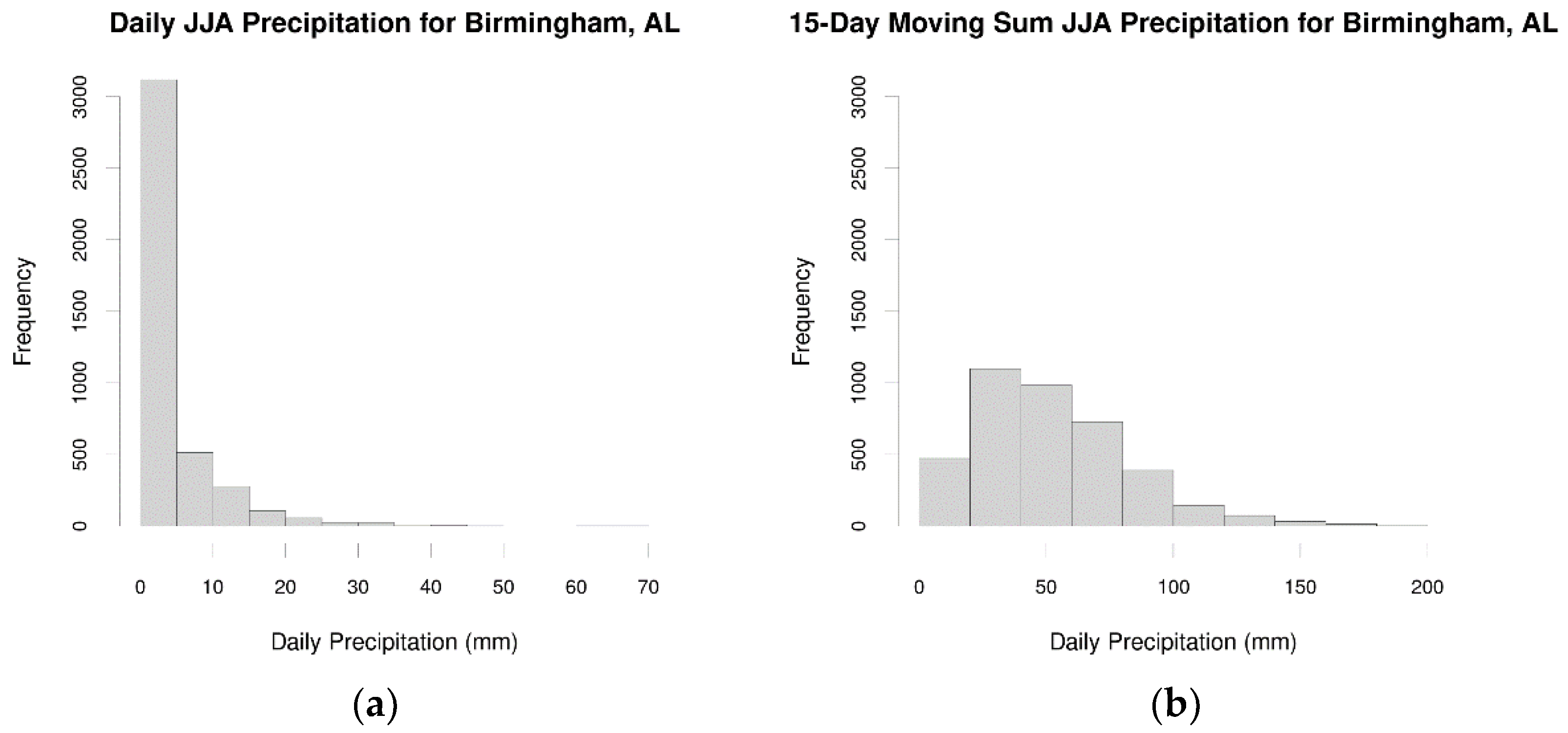
Figure 1. Daily precipitation (panel (a)) for NARR grid point nearest Birmingham, AL (33.24277° N, 86.79012° W) and 15-day moving sum of precipitation for the same grid point (panel (b)). Note the near elimination of the impacts of zeroes when employing the moving sum.
Climate 11 00002 g001
Figure 2. Mean precipitation (mm—panel (a)) and precipitation standard deviation (mm—panel (b)) for all 15-day moving sum data for the study domain.
Climate 11 00002 g002
Figure 3. Annual average (top panel) and standard deviation (bottom panel) 15-day moving sum precipitation for the full SEUS study domain. Information on the linear fit for each positive trend is provided in the respective top left corner of the panel.
Climate 11 00002 g003
Figure 4. Same as Figure 3, but for the detrended z-scores of precipitation mean (top panel) and standard deviation (bottom panel). Note that both trends are now nonsignificant (p = 0.93 for the means, p = 0.91 for the standard deviations).
Climate 11 00002 g004
Figure 5. Frequency of each cluster’s members by decade. The frequency of each cluster’s occurrence was highly consistent by decade with the exception of 1989–1998.
Climate 11 00002 g005
Figure 6. Cluster 1′s 15-day precipitation standard anomalies derived from KPCA-preprocessed cluster analysis. This pattern closely matched the composite with no KPCA-preprocessing, but 2005 was included as part of this cluster.
Climate 11 00002 g006
Figure 7. Cluster 2′s 15-day precipitation standard anomalies derived from KPCA-preprocessed cluster analysis. This pattern was slightly different than the one with no KPCA-preprocessing as 2005 was not included as part of this composite.
Climate 11 00002 g007
Figure 8. Cluster 3′s 15-day precipitation standard anomalies derived from KPCA-preprocessed cluster analysis. This pattern matched the cluster analysis with no KPCA-preprocessing.
Climate 11 00002 g008
Figure 9. Composite averages for clusters 1–3 (panels (ac)) of geopotential height (black contours—m), temperature (red dashed contours—K) and specific humidity (green dotted contours—g/kg) for 850 mb.
Climate 11 00002 g009
Figure 10. Oceanic Niño Index by year (top panel) and SEUS landfalling tropical cyclone frequency by year (bottom panel) for each cluster.
Climate 11 00002 g010
Figure 11. Precipitation anomalies for the 2005 warm season. Note the elevated precipitation along the Gulf Coast and into Georgia and the Carolinas coupled with the anomalously dry conditions in the northern and western portions of the study domain.
Climate 11 00002 g011
Table 1. Baseline cluster analysis (no KPCA) for each number of retained clusters.
Retained Clusters S ¯ Avg. Correlation
30.1050.763
40.0970.777
50.0960.790
60.0880.807
70.0970.812
80.0800.825
Table 2. Same as Table 1, but for the best KPCA configuration. No results for six or seven clusters outperformed the baseline, so the values were not provided. The loadings column refers to the number of retained loadings for the optimal KPCA configuration.
KernelLoadingsRetained Clusters S ¯ Avg. Correlation
Linear polynomial930.1050.765
RBF ( σ = 29 ) 2440.1000.788
RBF ( σ = 42 ) 2150.0970.794
RBF ( σ = 41 ) 3680.0810.829
Table 3. Bootstrap confidence intervals of 95% and medians for average annual SEUS landfalling tropical cyclones, broken down by cluster. If the median bootstrap replicate falls outside the interval for the other clusters, the difference was deemed statistically significant. Here, cluster 2 is significantly different than clusters 1 and 3, though clusters 1 and 3 are not statistically significantly different.
PercentileCluster 1Cluster 2Cluster 3
2.5%1.1580.6150.907
50%1.8951.0771.910
97.5%2.7371.6153.090
Disclaimer/Publisher’s Note: The statements, opinions and data contained in all publications are solely those of the individual author(s) and contributor(s) and not of MDPI and/or the editor(s). MDPI and/or the editor(s) disclaim responsibility for any injury to people or property resulting from any ideas, methods, instructions or products referred to in the content.