
Evaluation of the Urban Microclimate in Catania Using Multispectral Remote Sensing and GIS Technology


Abstract
:1. Introduction
2. Materials and Methods
2.1. Satellite Data
- Four bands with spatial resolution of 10 m.
- Six bands with spatial resolution of 20 m.
- Three bands with spatial resolution of 60 m.
2.2. Normalized Difference Vegetation Index
2.3. Weather Data
2.4. Land Surface Temperature
- M1 is the LST slope,
- M2 is the sum of the fixed and random Urban Percent slopes.
- M3 is the sum of the fixed and random elevation slopes.
- M4 is the sum of the fixed and random NDVI slopes.
- LST is the LSTHRES derived by Equation (6).
- Urban Percent is the percentage of urban area in the grid.
- Elevation is calculated from DEM (Digital Elevation Model).
- NDVI is the NDVIHRES.
- B is a datum obtained as the sum of the fixed intercepts and random intercepts.
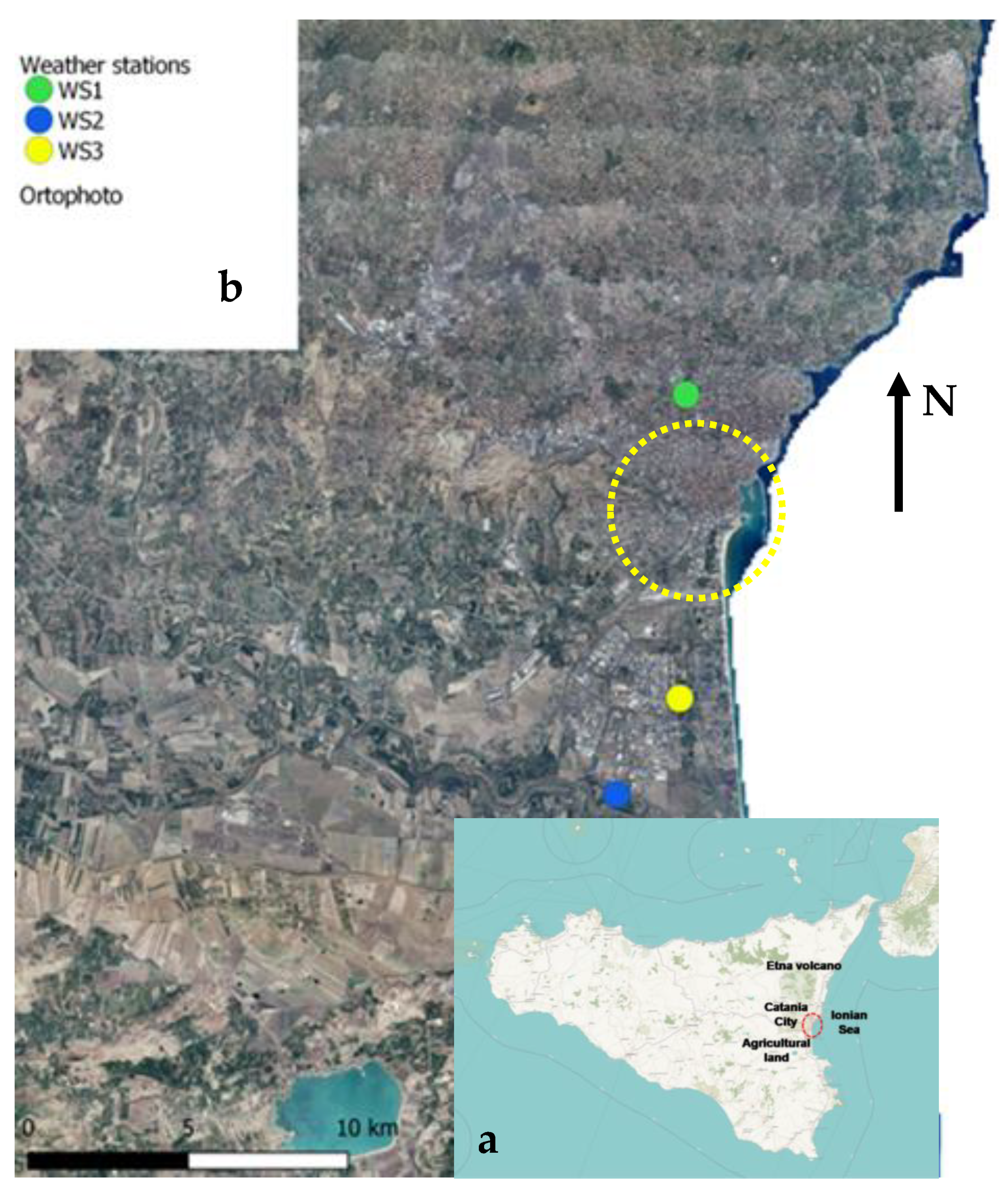
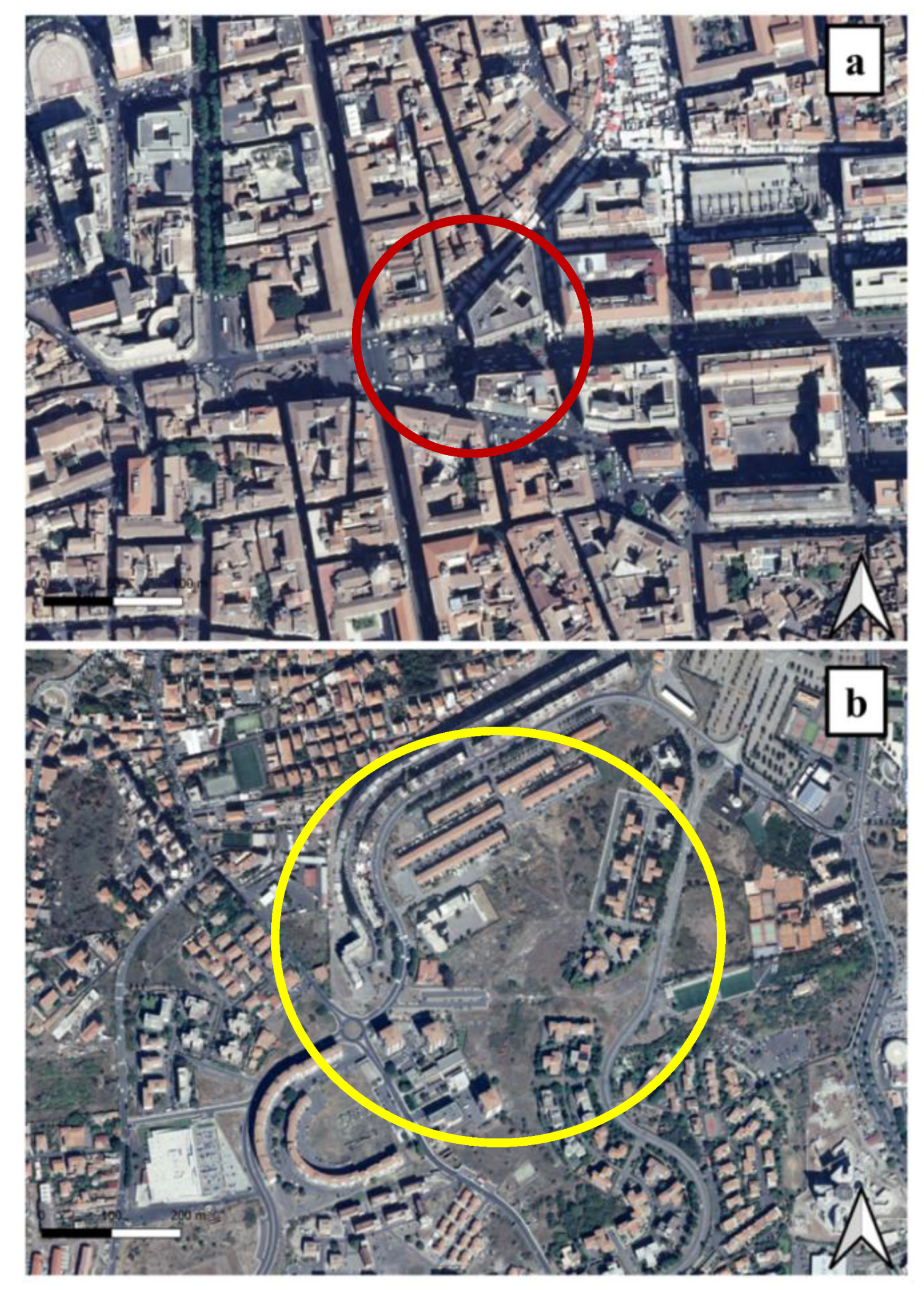
2.5. Case Study
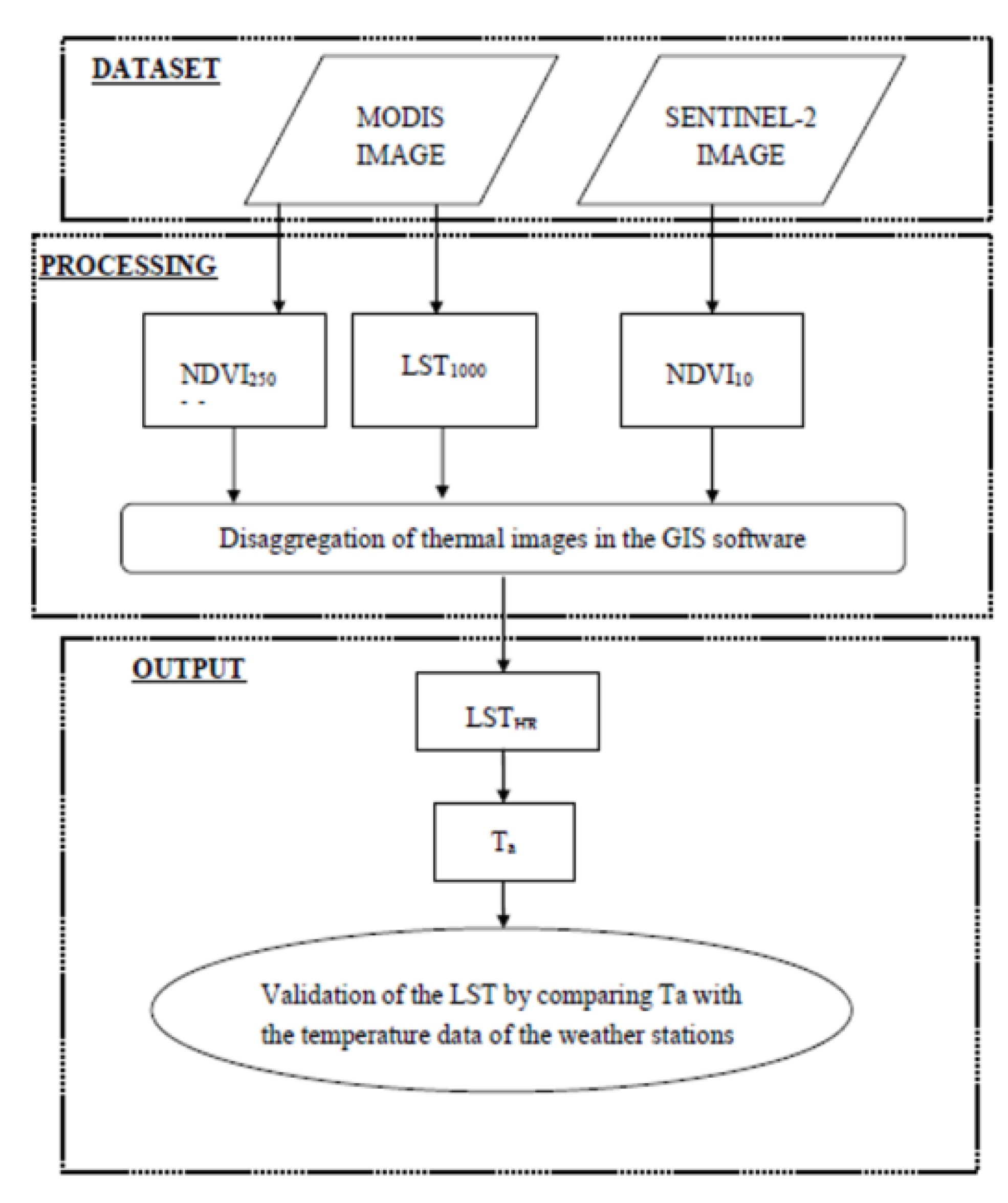
- Selection of the days to analyse based on the availability of both weather station and satellite data.
- Processing of MODIS and SENTINEL-2 satellite images in a GIS environment.
- Application to the investigated area.
- Analysis of the atmospheric temperatures.
3. Results
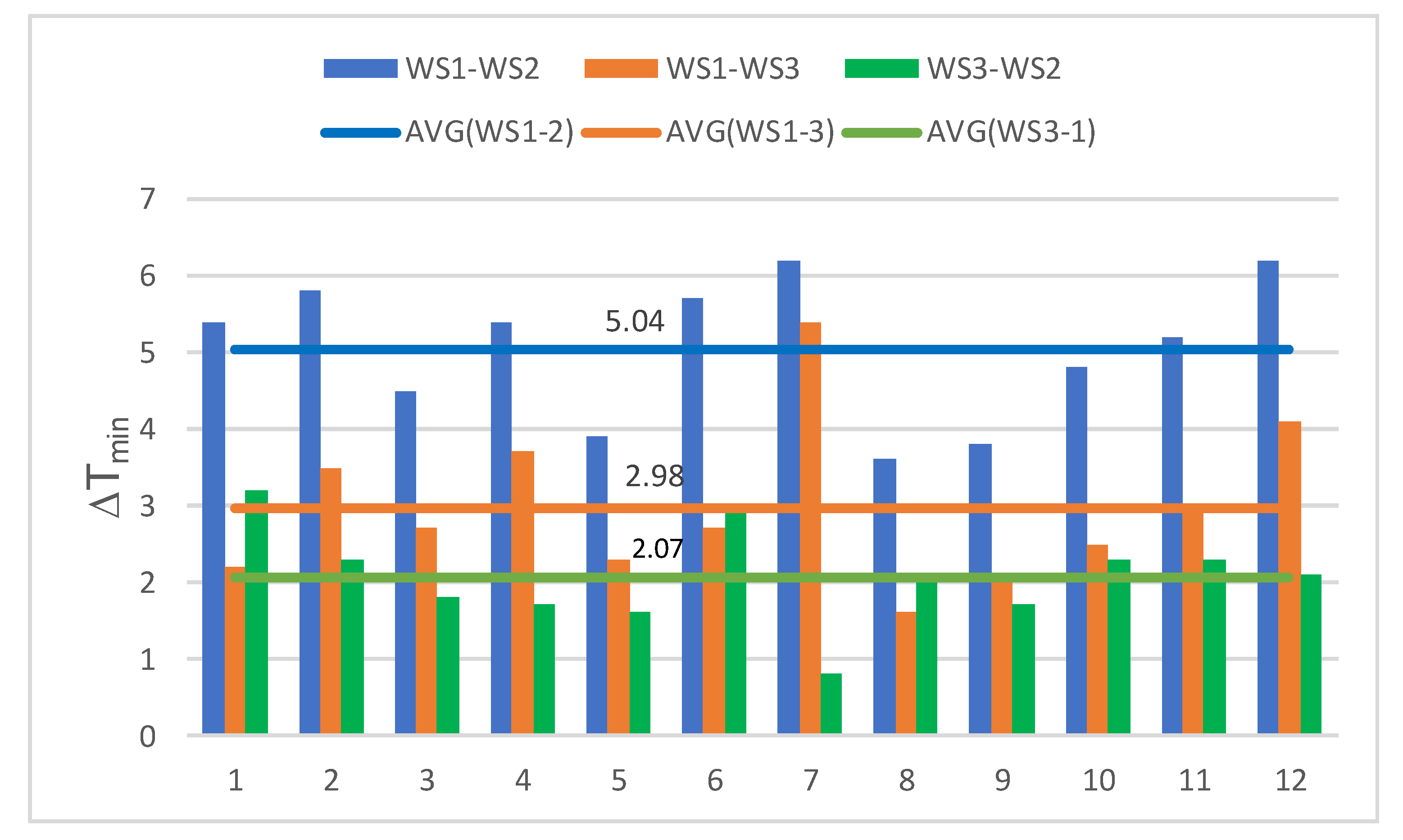
3.1. Data Measured by the Weather Stations
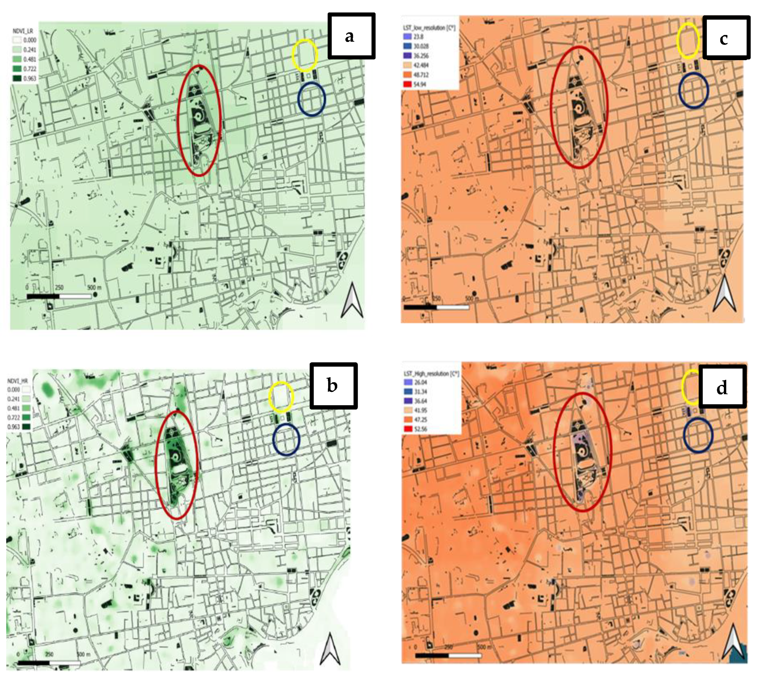
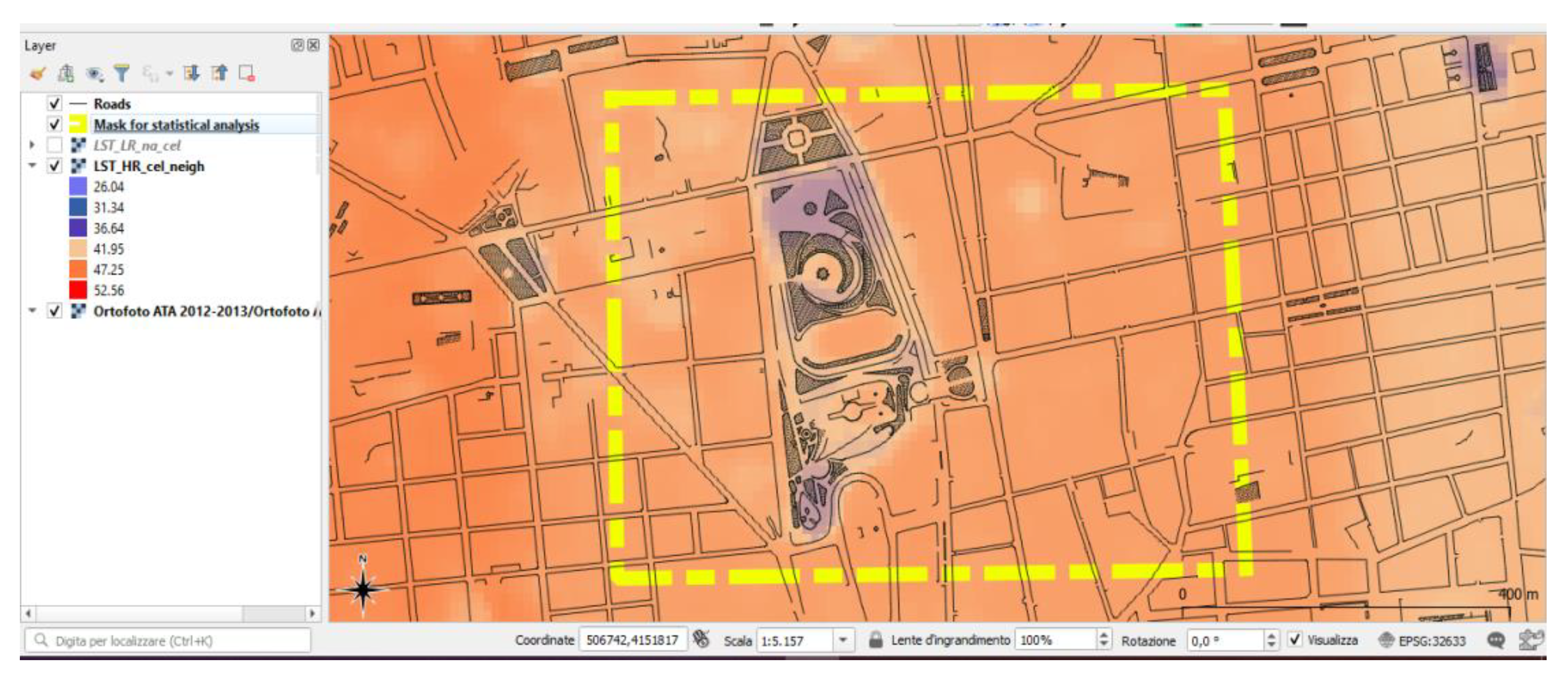
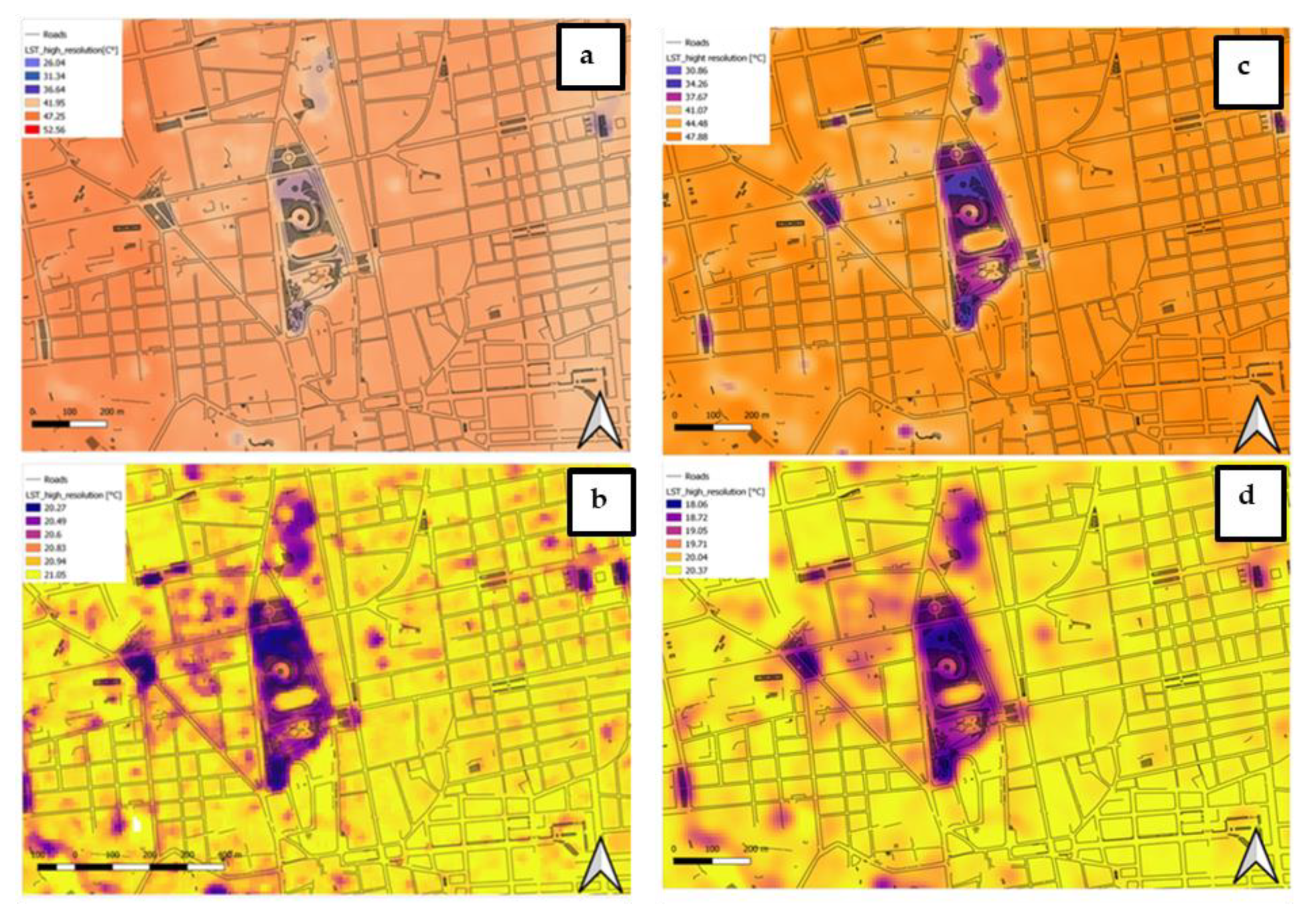
3.2. NDVI and LST Derived by Satellite Images
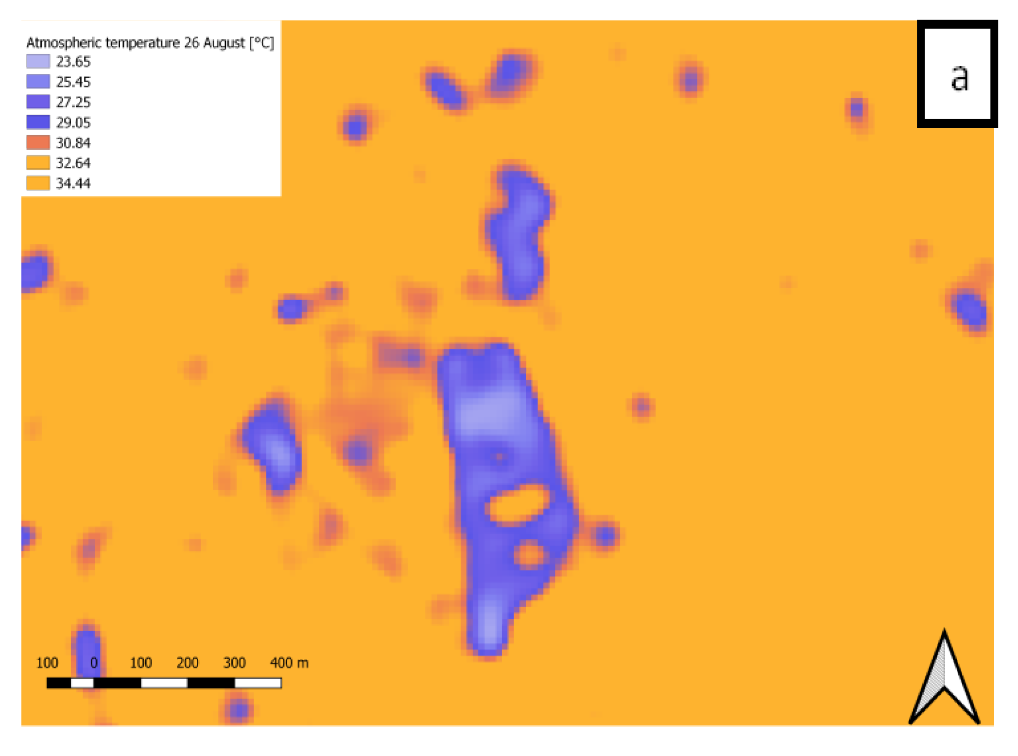
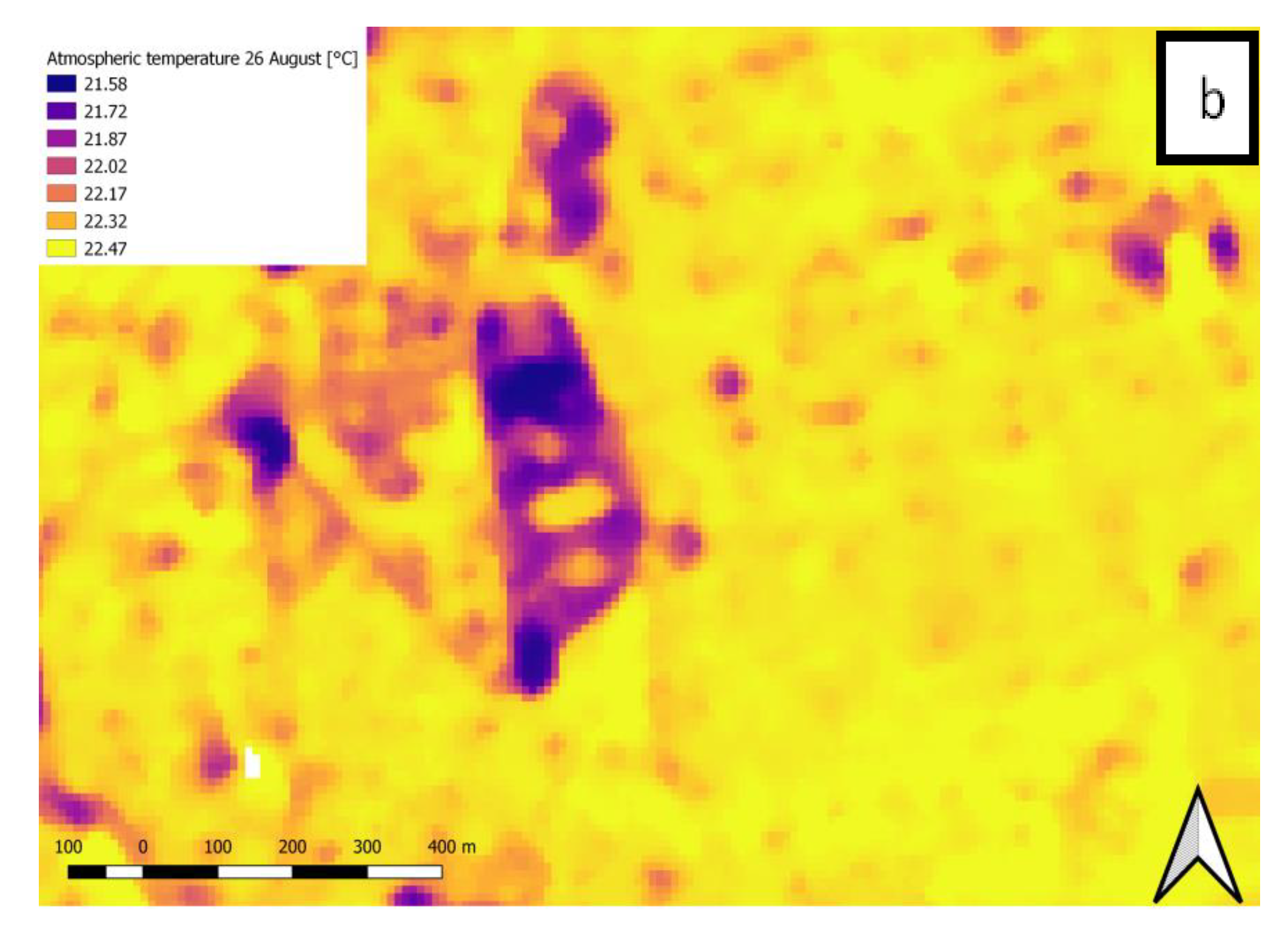
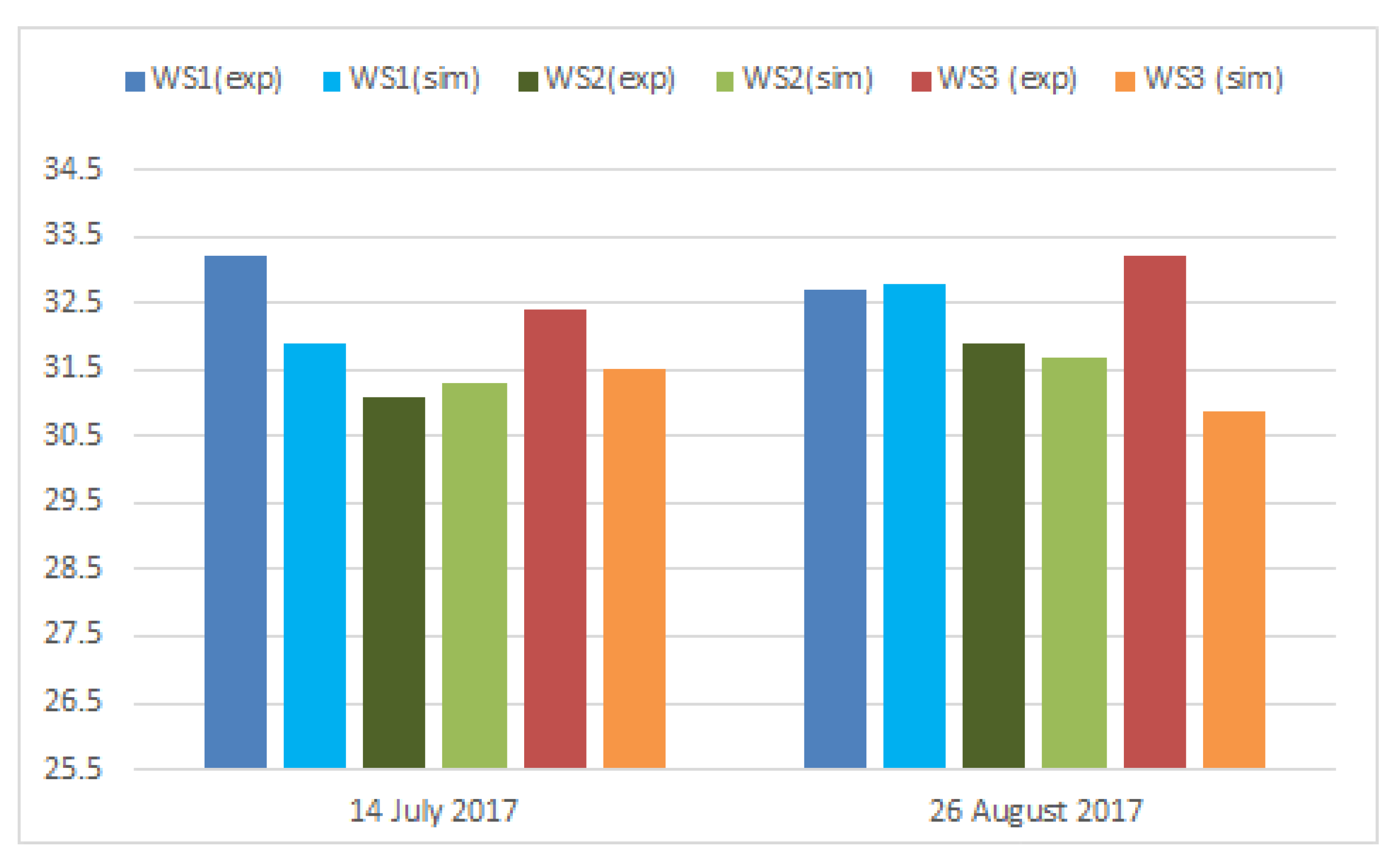
3.3. Atmospheric Temperature
4. Discussion
Author Contributions
Funding
Data Availability Statement
Acknowledgments
Conflicts of Interest
References
- Zeng, Y.; Huang, W.; Zhan, F.B.; Zhang, H.; Liu, H. Study on the urban heat island effects and its relationship with surface biophysical characteristics using MODIS imageries. Geo Spat. Inf. Sci. 2010, 13, 1–7. [Google Scholar] [CrossRef] [Green Version]
- Shahmohamadi, P.; Che-Ani, A.I.; Etessam, I.; Maulud, K.N.A.; Tawil, N.M. Healthy environment: The need to mitigate urban heat island effects on human health. Proc. Eng. 2011, 20, 61–70. [Google Scholar] [CrossRef] [Green Version]
- Heaviside, C.; Macintyre, H.; Vardoulakis, S. The urban heat island: Implications for health in a changing environment. Curr. Environ. Health Rep. 2017, 4, 296–305. [Google Scholar] [CrossRef] [PubMed]
- Gagliano, A.; Nocera, F.; Aneli, S. Computational fluid dynamics analysis for evaluating the urban heat island effects. Energy Procedia 2017, 134, 508–517. [Google Scholar] [CrossRef]
- Cascone, S.; Catania, F.; Gagliano, A.; Sciuto, G. A comprehensive study on green roof performance for retrofitting existing buildings. Build. Environ. 2018, 136, 227–239. [Google Scholar] [CrossRef]
- Jiang, D.; Huang, S.; Han, D. Monitoring and modelling terrestrial ecosystems response to climate change. Adv. Meterology 2014, 2014, 374987. [Google Scholar] [CrossRef]
- Ahmed, S. Assessment of urban heat islands and impact of climate change on socioeconomic over Suez governorate using remote sensing and GIS techniques. Egypt. J. Remote Sens. Space Sci. 2018, 21, 15–25. [Google Scholar] [CrossRef]
- Unger, J. Connection between urban heat island and sky view factor approximated by a software tool on a 3D urban database. Int. J. Environ. Pollut. 2009, 36, 59. [Google Scholar] [CrossRef] [Green Version]
- U.S. Environmental Protection Agency. Reducing Urban Heat Islands: Compendium of Strategies. Draft. 2008. Available online: https://www.epa.gov/heat-islands/heat-island-compendium (accessed on 21 April 2020).
- Susca, T.; Gaffin, S.R.; Dell’Osso, G.R. Positive effects of vegetation: Urban heat island and green roofs. Environ. Pollut. 2011, 159, 2119–2126. [Google Scholar] [CrossRef]
- Xie, P.; Wang, H. Potential benefit of photovoltaic pavement for mitigation of urban heat island effect. Appl. Therm. Eng. 2021, 191, 116883. [Google Scholar] [CrossRef]
- Li, H.; Harvey, J.T.; Holland, T.J.; Kayhanian, M. The use of reflective and permeable pavements as a potential practice for heat island mitigation and storm water management. Environ. Res. Lett. 2013, 8, 015023. [Google Scholar] [CrossRef]
- Mohajerani, A.; Bakaric, J.; Jeffrey-Bailey, T. The urban heat island effect, its causes, and mitigation, with reference to the thermal properties of asphalt concrete. J. Environ. Manag. 2017, 197, 522–538. [Google Scholar] [CrossRef] [PubMed]
- Cortes, A.; Murashita, Y.; Matsuo, T.; Kondo, A.; Shimadera, H.Y. Numerical evaluation of the effect of photovoltaic cell installation on urban thermal environment. Sustain. Cities Soc. 2015, 19, 250–258. [Google Scholar] [CrossRef]
- Cilek, M.U.; Cilek, A. Analyses of land surface temperature (LST) variability among local climate zones (LCZs) comparing Landsat-8 and ENVI-met model data. Sustain. Cities Soc. 2021, 69, 102877. [Google Scholar] [CrossRef]
- Mutiibwa, D.; Strachan, S.; Albright, T. Land surface temperature and surface air temperature in complex terrain. IEEE J. Select. Topics Appl. Earth Observat. Remote Sens. 2015, 8, 4762–4774. [Google Scholar] [CrossRef]
- Mejbel Salih, M.; Zakariya Jasim, O.; Hassoon, K.I.; Jameel Abdalkadhum, A. Land surface temperature retrieval from LANDSAT-8 thermal infrared sensor data and validation with infrared thermometer camera. Int. J. Eng. Technol. 2018, 7, 608. [Google Scholar] [CrossRef] [Green Version]
- Algretawee, H.; Rayburg, S.; Neave, M. Estimating the effect of park proximity to the central of Melbourne city on Urban Heat Island (UHI) relative to Land Surface Temperature (LST). Ecol. Eng. 2019, 138, 374–390. [Google Scholar] [CrossRef]
- Jin, M.; Dickinson, R.E. Land surface skin temperature climatology: Benefitting from the strengths of satellite observations. Environ. Res. Lett. 2010, 5, 044004. [Google Scholar] [CrossRef] [Green Version]
- Qin, Z.H.; Karnieli, A.; Berliner, P. A mono-window algorithm for retrieving land surface temperature from Landsat TM data and its application to the Israel-Egypt border region. Int. J. Remote Sens. 2001, 22, 3719–3746. [Google Scholar] [CrossRef]
- Otaghsara, M.P.T.; Arefi, H. Modelling urban heat island using remote sensing and city morphological parameters. In Proceedings of the International Archives of the Photogrammetry, Remote Sensing and Spatial Information Sciences, Karaj, Iran, 12–14 October 2019; International Society of Photogrammetry and Remote Sensing (ISPRS): Nice, France, 2019; Volume XLII-4/W18. [Google Scholar]
- Mamdouh, E.H.; Amany, S.M.; Lamia, G.E. Monitoring and assessment of urban heat islands over the Southern region of Cairo Governorate. Egypt. Egypt. J. Remote Sens. Space Sci. 2018, 21, 311–323. [Google Scholar]
- Katsoulis, B.D.; Theoharatos, G.A. Indications of urban heat island in Athens, Greece. Appl. Meteorol. 1985, 24, 1296–1302. [Google Scholar] [CrossRef] [Green Version]
- Gagliano, A.; Patania, F.; Nocera, F.; Capizzi, A.; Galesi, A. GIS-based decision support for solar photovoltaic planning in urban environment. In Sustainability in Energy and Buildings; Springer: Berlin/Heidelberg, Germany, 2013; pp. 865–874. [Google Scholar]
- Mineo, S.; Pappalardo, G.; Mangiameli, M.; Campolo, S.; Mussumeci, G. Rockfall Analysis for Preliminary Hazard Assessment of the Cliff of Taormina Saracen Castle (Sicily). Sustainability 2018, 10, 417. [Google Scholar] [CrossRef] [Green Version]
- Gennaro, A.; Candiano, A.; Fargione, G.; Mangiameli, M.; Mussumeci, G. Multispectral remote sensing for post--dictive analysis of archaeological remains. A case study from Bronte (Sicily). Archaelogical Prospect. 2019, 26, 299–311. [Google Scholar] [CrossRef]
- Gennaro, A.; Candiano, A.; Fargione, G.; Mussumeci, G.; Mangiameli, M. GIS and remote sensing for post-dictive analysis of archaeological features. A case study from the Etnean region (Sicily). Archeol. Calc. 2019, 30, 309–328. [Google Scholar] [CrossRef]
- Mangiameli, M.; Mussumeci, G. Gis approach for preventive evaluation of roads loss of efficiency in hydrogeological emergencies, 2013, International Archives of the Photogrammetry. In Proceedings of the Remote Sensing and Spatial Information Sciences—ISPRS Archives, Padua, Italy, 27–28 February 2013; ISPRS: Nice, France, 2013; Volume 40, pp. 79–87. [Google Scholar]
- Mangiameli, M.; Mussumeci, G.; Candiano, A. A low cost methodology for multispectral image classification. In Proceedings of the 18th International Conference on Computational Science and Its Applications, Melbourne, VIC, Australia, 2–5 July 2018; ICCSA: Melbourne, VIC, Australia, 2018; Volume 10964, pp. 263–280. [Google Scholar]
- Equere, V.; Mirzaei, P.A.; Riffa, S.; Wang, Y. Integration of topological aspect of city terrains to predict the spatial distribution of urban heat island using GIS and ANN. Sustain. Cities Soc. 2021, 69, 102825. [Google Scholar] [CrossRef]
- Zhou, X.; Okaze, T.; Ren, C.; Cai, M.; Ishida, Y.; Watanabe, H.; Mochida, A. Evaluation of urban heat islandsusing local climate zones and the influence of sea-land breeze. Sustain. Cities Soc. 2020, 55, 102060. [Google Scholar] [CrossRef]
- Bauer, T.J. Interaction of urban heat island e_ects and land–sea breezes during a new york city heat event. J. Appl. Meteorol. Climatol. 2020, 59, 477–495. [Google Scholar] [CrossRef]
- Papanastasiou, D.K.; Melas, D.; Bartzanas, T.; Kittas, C. Temperature, comfort and pollution levels duringheat waves and the role of sea breeze. Int. J. Biometeorol. 2010, 54, 307–317. [Google Scholar] [CrossRef]
- Freitas, E.D.; Rozo, C.M.; Cotton, W.R.; Silva Dias, P.L. Interactions of an urban heat island and sea-breeze circulations during winter over the metropolitan area of São Paulo, Brazil. Bound. Layer Meteorol. 2007, 122, 43–65. [Google Scholar] [CrossRef]
- Martinelli, A.; Kolokotsa, D.D.; Fiorito, F. Urban heat island in Mediterranean coastal cities: The case of Bari (Italy). Climate 2020, 8, 79. [Google Scholar] [CrossRef]
- Kang, X.; Huiping, X. RS and GIS-based analysis of urban heat island effect in Shanghai. In Proceedings of the 18th International Conference on Geoinformatics, Beijing, China, 18–20 June 2010; IEEE: Piscataway, NJ, USA, 2010. [Google Scholar] [CrossRef]
- Viana, C.M.; Oliveira, S.; Oliveira, S.C.; Rocha, J. Land Use/Land Cover Change Detection and Urban Sprawl Analysis. In Spatial Modeling in GIS and R for Earth and Environmental Sciences; Elsevier: Amsterdam, The Netherlands, 2019; pp. 621–651. [Google Scholar] [CrossRef]
- Baghdadi, N.; Mallet, C.; Zribi, M. QGIS and Applications in Agriculture and Forest; Wiley Blackwell: Hoboken, NJ, USA, 2018; Volume 3, pp. 1–270. [Google Scholar] [CrossRef]
- Li, Z.L.; Tang, B.H.; Wu, H.; Ren, H.; Yan, G.; Wan, Z.; Trigo, I.F.; Sobrino, J.A. Satellite-derived land surface temperature: Current status and perspectives. Remote Sens. Environ. 2013, 131, 14–37. [Google Scholar] [CrossRef] [Green Version]
- Sobrino, J.A.; ElKharraz, J.; Li, Z.L. Surface temperature and water vapour retrieval from MODIS data. Int. J. Remote Sens. 2003, 24, 5161–5182. [Google Scholar] [CrossRef]
- Pettorelli, N. The Normalized Difference Vegetation Index; Oxford University Press: Oxford, UK, 2013. [Google Scholar]
- Bisquert, M.; Sánchez, T.; Juan, M.; Caselles, V. Evaluation of Disaggregation Methods for Downscaling MODIS Land Surface Temperature to Landsat Spatial Resolution in Barrax Test Site. IEEE J. Sel. Top. Appl. Earth Obs. Remote Sens. 2016, 9, 1430–1438. [Google Scholar] [CrossRef]
- Liu, S.; Su, H.; Zhang, R.; Tian, J.; Wang, W. Estimating the surface air temperature by remote sensing in Northwest China using an improved advection-energy balance for air temperature model. Adv. Meteorol. 2016, 2016, 11. [Google Scholar] [CrossRef] [Green Version]
- Alqasemi, A.S.; Hereher, M.E.; Al-Quraishi, A.M.F.; Saibid, H.; Aldahan, A.; Abuelgasim, A. Retrieval of monthly maximum and minimum air temperature using MODIS aqua land surface temperature data over the United Arab Emirates. Geocarto Int. 2020, 767, 144330. [Google Scholar] [CrossRef]
- Kloog, I.; Nordio, F.; Coull, B.A.; Schwartz, J. Predicting spatiotemporal mean air temperature using MODIS satellite surface temperature measurements across the Northeastern USA. Remote Sens. Environ. 2014, 150, 132–139. [Google Scholar] [CrossRef]
- City of Cambridge. Massachusetts Climate Change Vulnerability Assessment November 2015; Appendix D: Urban Heat Island Protocol for Mapping Temperature Projections; City of Cambridge: Cambridge, MS, USA, 2015.
- Colston, J.M.; Ahmed, T.; Mahopo, C.; Kang, G.; Kosek, M.; de Sousa, F., Jr.; Shrestha, P.S.; Svensen, E.; Turab, A.; Zaitchik, B. Evaluating meteorological data from weather stations, and from satellites and global models for a multi-site epidemiological study. Environ. Res. 2018, 165, 91–109. [Google Scholar] [CrossRef]
- Giannaros, T.M.; Melas, D. Study of the urban heat island in a coastal Mediterranean City: The case study of Thessaloniki, Greece. Atmos. Res. 2012, 118, 103–120. [Google Scholar] [CrossRef]
- Battista, G.; Evangelisti, L.; Guattari, C.; Vollaro, E.D.L.; Vollaro, R.D.L.; Asdrubali, F. Urban Heat Island Mitigation Strategies: Experimental and Numerical Analysis of a University Campus in Rome (Italy). Sustainability 2020, 12, 7971. [Google Scholar] [CrossRef]
- Georgakis, C.; Santamouris, M. Determination of the Surface and Canopy Urban Heat Island in AthensCentral Zone Using Advanced Monitoring. Climate 2017, 5, 97. [Google Scholar] [CrossRef] [Green Version]
- Giannopoulos, A.; Caouris, Y.G.; Souliotis, M.; Sntamouris, M. Characteristics of the urban heat island effect, in the coastal city of Patras, Greece. Int. J. Sustain. Energy 2021, 0, 1–16. [Google Scholar] [CrossRef]


| Days | Daytime | Nighttime |
|---|---|---|
| 4 July 2017 | 10:36 | 21:36 |
| 9 July 2017 | 10:54 | 22:00 |
| 12 July 2017 | 11:24 | 22:20 |
| 14 July 2017 | 11:12 | 22:18 |
| 22 July 2017 | 10:24 | 21:30 |
| 29 July 2017 | 10:30 | 21:36 |
| 3 August 2017 | 10:48 | 21:54 |
| 11 August 2017 | 11:36 | 22:42 |
| 16 August 2017 | 10:18 | 21:18 |
| 18 August 2017 | 11:42 | 22:48 |
| 26 August 2017 | 10:54 | 22:00 |
| 28 August 2017 | 10:42 | 21:48 |
| Days | WS1-DIEEI (Lat 37.525, Long 15.072) | WS2-ENEL (Lat 37.414, Long 15.047) | WS3-SIAS (Lat 37.441, Long 15.069) | ||||||
|---|---|---|---|---|---|---|---|---|---|
| Tmax | Tmin | Tavg | Tmax | Tmin | Tavg | Tmax | Tmin | Tavg | |
| 4 July 2017 | 29.2 | 22.0 | 25.9 | 31.5 | 16.6 | 25.6 | 29.7 | 19.8 | 25.5 |
| 9 July 2017 | 36.8 | 24.7 | 30.5 | 36.1 | 18.9 | 27.6 | 34.2 | 24.7 | 27.5 |
| 12 July 2017 | 39.9 | 28.2 | 33.3 | 42.1 | 23.7 | 31.2 | 40.8 | 25.5 | 31.7 |
| 14 July 2017 | 33.2 | 25.3 | 29.1 | 32.4 | 19.9 | 27.1 | 31.1 | 21.6 | 27.1 |
| 22 July 2017 | 36.2 | 25.8 | 31.7 | 40.0 | 21.9 | 30.8 | 37.9 | 23.5 | 31.3 |
| 29 July 2017 | 33.3 | 23.3 | 27.2 | 32.1 | 17.6 | 25.6 | 30.7 | 20.6 | 25.6 |
| 3 August 2017 | 37.5 | 26.4 | 32.1 | 39.1 | 20.2 | 28.8 | 34.2 | 21.2 | 28.8 |
| 11 August 2017 | 35.3 | 26.4 | 31.2 | 35.3 | 22.8 | 28.8 | 34.2 | 24.8 | 29.0 |
| 16 August 2017 | 31.6 | 23.7 | 27.6 | 31.9 | 19.9 | 26.3 | 30.9 | 21.6 | 26.9 |
| 18 August 2017 | 32.8 | 24.1 | 28.7 | 34.1 | 19.3 | 27.0 | 33.5 | 21.6 | 27.4 |
| 26 August 2017 | 32.7 | 23.9 | 27.8 | 33.2 | 18.7 | 25.9 | 31.9 | 21.0 | 26.2 |
| 28 August 2017 | 32.2 | 24.1 | 28.2 | 33.0 | 17.9 | 26.0 | 31.1 | 20.0 | 26.2 |
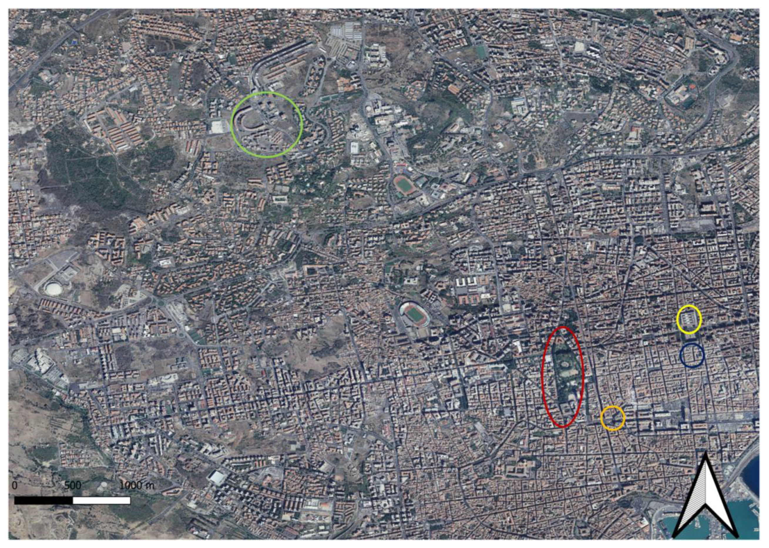
| Daytime Temperature on 14 July | Daytime Temperature on 26 August | Nighttime Temperature on 14 July | Nighttime Temperature on 26 August | |
|---|---|---|---|---|
| Villa Bellini | 29 | 31 | 20 | 18 |
| Skyscraper | 45 | 44 | 21 | 20 |
| Courthouse | 42 | 45 | 21 | 20 |
Publisher’s Note: MDPI stays neutral with regard to jurisdictional claims in published maps and institutional affiliations. |
© 2022 by the authors. Licensee MDPI, Basel, Switzerland. This article is an open access article distributed under the terms and conditions of the Creative Commons Attribution (CC BY) license (https://creativecommons.org/licenses/by/4.0/).
Share and Cite
Mangiameli, M.; Mussumeci, G.; Gagliano, A. Evaluation of the Urban Microclimate in Catania Using Multispectral Remote Sensing and GIS Technology. Climate 2022, 10, 18. https://doi.org/10.3390/cli10020018
Mangiameli M, Mussumeci G, Gagliano A. Evaluation of the Urban Microclimate in Catania Using Multispectral Remote Sensing and GIS Technology. Climate. 2022; 10(2):18. https://doi.org/10.3390/cli10020018
Chicago/Turabian StyleMangiameli, Michele, Giuseppe Mussumeci, and Antonio Gagliano. 2022. "Evaluation of the Urban Microclimate in Catania Using Multispectral Remote Sensing and GIS Technology" Climate 10, no. 2: 18. https://doi.org/10.3390/cli10020018
APA StyleMangiameli, M., Mussumeci, G., & Gagliano, A. (2022). Evaluation of the Urban Microclimate in Catania Using Multispectral Remote Sensing and GIS Technology. Climate, 10(2), 18. https://doi.org/10.3390/cli10020018