Does the Choice of Realized Covariance Measures Empirically Matter? A Bayesian Density Prediction Approach

Abstract

This paper suggests a new approach to evaluate realized covariance (RCOV) estimators via their predictive power on return density. By jointly modeling returns and RCOV measures under a Bayesian framework, the predictive density of returns and ex-post covariance measures are bridged. The forecast performance of a covariance estimator can be assessed according to its improvement in return density forecasting. Empirical applications to equity data show that several RCOV estimators consistently perform better than others and emphasize the importance of RCOV selection in covariance modeling and forecasting.

1. Introduction

The past two decades have seen dramatic growth in the amount of literature on estimating and modeling realized covariance (RCOV) measures. On the one hand, various methods have been proposed to extract covariation information from noisy and non-synchronous high-frequency data. On the other hand, the literature on RCOV modeling has focused on improving models’ flexibility and predictability. Which RCOV measure leads to superior out-of-sample forecasting is an important but not fully answered question. This paper suggests a joint return and RCOV modeling approach to assess RCOV measures based on return density forecasts. This direction of research contributes not only to the ex-post covariance estimation literature by proposing a new evaluation method but also to the RCOV modeling literature as we show that the choice of estimator matters to a model’s predictability.

Most studies regarding ex-post covariance estimation focus on developing a high-frequency covariance estimator that can accommodate market microstructure noise and non-synchronous trading without losing consistency and efficiency. Andersen et al. (2003) and Barndorff-Nielsen and Shephard (2004) build the theoretical foundation of RCOV in an ideal setting. Zhang et al. (2005) suggest the subsampling approach and Zhang (2011) designs a two-scales realized covariance (TSRC). Griffin and Oomen (2011) analyze the statistical properties of RCOV with lead-lag adjustments (RCLL). Barndorff-Nielsen et al. (2011) design a multivariate realized kernel (RK) based on refresh-time based returns. Christensen et al. (2010) extend the idea of pre-averaging in Jacod et al. (2009) to the multivariate setting and propose pre-averaged covariance estimators. Aït-Sahalia et al. (2010) introduce a quasi-maximum likelihood approach to estimate the ex-post covariance. Other estimation methods include those of Hayashi and Yoshida (2005), Voev and Lunde (2007), Hansen et al. (2008), Bannouh et al. (2009), Tao et al. (2011), Corsi et al. (2015), Peluso et al. (2015) and Lunde et al. (2016).

A common practice for assessing the accuracy of covariance estimators is via simulation-based exercises. For example, works by Voev and Lunde (2007), Jacod et al. (2009), Aït-Sahalia et al. (2010), Barndorff-Nielsen et al. (2011), Corsi et al. (2015), and Peluso et al. (2015) compare several RCOV estimators via simulation studies. This approach is useful in studying estimation accuracy and efficiency but cannot evaluate estimators’ empirica performance.

An alternative RCOV evaluation approach is based on out-of-sample portfolio performance. For example, among competing covariance estimators, the estimator that leads to the least volatile minimum-variance portfolio is preferred. In the context of portfolio optimization, de Pooter et al. (2008) evaluate the choice of sampling frequency in constructing RCOVs. Fan et al. (2012) study covariance matrix estimation from the perspective of portfolio selection with gross-exposure constraints. Corsi et al. (2015) and Lunde et al. (2016) conduct portfolio allocation experiments to compare their proposed estimators with benchmarks. Compared with statistical evaluation based on simulation studies, the mean-variance portfolio optimization provides an indirect criterion for assessing estimator performance from an economic perspective.

Recent developments in RCOV modeling facilitate the application of realized measures to forecast future covariance. Gourieroux et al. (2009) pioneer RCOV modeling by suggesting a non-central Wishart distribution to accommodate the positivity and symmetry of RCOV measures. Golosnoy et al. (2012) introduce a conditional autoregressive Wishart (CAW) model, and Yu et al. (2017) suggest a generalized CAW. Jin and Maheu (2013) propose a class of joint return-RCOV models based on Wishart distributions with additive or multiplicative components. Chiriac and Voev (2010), Bauer and Vorkink (2011) and Cech and Barunik (2017) apply standard time-series methods to model transformations of RCOV. Hansen et al. (2014) propose a multivariate GARCH model incorporating RCOV measures. Noureldin et al. (2012) design a multivariate high-frequency volatility (HEAVY) model and Opschoor et al. (2018) extend the HEAVY model to allow for better fitting. Jin and Maheu (2016) introduce a Bayesian nonparametric framework for RCOV modeling. Asai and McAleer (2015), Jin et al. (2019) and Shen et al. (2020) design factor models for RCOV. Amendola et al. (2020) propose a strategy based on the model confidence set to evaluate a group of multivariate volatility models. The literature surrounding RCOV modeling emphasizes the flexibility and predictability of models, while the practical importance of selecting RCOV measures has typically been ignored. In most works, RCOV constructed using low-frequency returns and realized kernel are the main choices of ex-post covariance measures.

Investigating the predictive power of RCOV measures is important to both academia and industry. However, directly measuring the accuracy of covariance prediction is infeasible as volatility is unobservable. In a univariate setting, Aït-Sahalia and Mancini (2008) rely on simulated data to compare out-of-sample forecasts of two realized volatility (RV) estimators. This paper suggests an approach based on return density forecasts to evaluate RCOV estimators. Our approach is inspired by several works on joint return-RCOV modeling, such as Noureldin et al. (2012), Jin and Maheu (2013) and Jin and Maheu (2016). By jointly modeling returns and RCOV measures under a Bayesian framework, the predictive density of returns and ex-post covariance measures are bridged, which allows the use of observed returns as the criterion for evaluating RCOV estimators. The density forecast improvement offered by a covariance estimator can be quantified using the predictive likelihood of returns. We evaluate a group of RCOV estimators using three joint return-RCOV models with different specifications. Empirical results support that the density-forecast-based method is an efficient way of assessing the out-of-sample performance of RCOV estimators. Our results also show that with regard to the pursuit of better predictability, the choice of RCOV estimator is as important as the model specification.

Compared with the evaluation method based on portfolio allocation, the density-forecast-based approach requires stochastic assumptions on returns and RCOV estimates, but offers several advantages. First, predictive likelihood reflects the accuracy of forecasting the return distribution. In contrast, portfolio analysis typically only considers the first two moments of the distribution. Second, portfolio exercise requires a reasonable long out-of-sample period to summarize portfolio performance, whereas the predictive likelihood measures the density forecast at each period and is not sensitive to the out-of-sample size. Third, forming a portfolio reduces the data dimension from multivariate to univariate. As a result, the difference among various RCOV measures may be averaged out and not be revealed based on portfolio returns. In contrast, the density forecast approach directly uses return vectors as the criterion, which reduces potential information loss. Overall, the density-forecast-based approach offers a direct and improved way to evaluate the out-of-sample performance of RCOV measures.

This paper is organized as follows. Section 2 provides a review of seven commonly used ex-post covariance estimation approaches. Section 3 discusses joint return-RCOV models, prediction and comparison criteria. Section 4 summarizes the data. Empirical results are reported in Section 5. Section 6 concludes, followed by an Appendix A.

2. Review of Ex-Post Covariance Estimation

Suppose the d dimensional log price follows a continuous stochastic process

$$\mathrm{d}P\left(t\right)=m\left(t\right)dt+\mathsf{\Pi }\left(t\right)dw\left(t\right),$$

(1)

where $m\left(t\right)$ is a $d\times 1$ vector of drift terms, $\mathsf{\Pi }\left(t\right)$ is a $d\times d$ instantaneous volatility matrix and $w\left(t\right)$ is a $d\times 1$ vector of standard Brownian motions. As shown in Andersen et al. (2003),

$$P\left(t\right)-P\left(0\right)\sim N\left({\int }_0^{t}m\left(\tau \right)d\tau ,{\int }_0^t\mathsf{\Pi }\left(\tau \right)\mathsf{\Pi }{\left(\tau \right)}^{\prime }d\tau \right),$$

(2)

where ${\int }_0^t\mathsf{\Pi }\left(\tau \right)\mathsf{\Pi }{\left(\tau \right)}^{\prime }\mathrm{d}\tau$ is the quadratic covariation which measures the covariance of the log return over time $(0,t)$.

Let ${\tilde{p}}_{t,{\tau }_l^{\left(j\right)}}^{\left(j\right)},l=1,\cdots ,n_t^{\left(j\right)}$, denotes the $l^{th}$ observed intraday price of asset j, where ${\tau }_l^{\left(j\right)}$ represents its arrival time and $n_t^{\left(j\right)}$ is the number of observations on day t. For most high-frequency covariance estimators, data synchronization is required. Under the previous-tick scheme with grid length h, regularly-spaced log prices are sampled as

$$p_{t,i}^{\left(j\right)}={\tilde{p}}_{t,max\left({\tau }_l^{\left(j\right)}\right|{\tau }_l^{\left(j\right)}\le ih)}^{\left(j\right)},j=1,\cdots ,d.$$

(3)

Let $R_{t,i}=(r_{t,i}^{\left(1\right)},r_{t,i}^{\left(2\right)},\cdots ,r_{t,i}^{\left(d\right)})$, where $r_{t,i}^{\left(j\right)}=p_{t,i}^{\left(j\right)}-p_{t,i-1}^{\left(j\right)}$, represents the intraday return vector over time $\left(\right(i-1)h,ih)$ on day t.

An alternative data synchronization approach is the refresh time scheme proposed by Barndorff-Nielsen et al. (2011), under which prices are sampled when all asset prices are refreshed. The $i^{th}$ refreshed price ${\dot{p}}_{t,i}^{\left(j\right)}$ is sampled as

$${\dot{p}}_{t,i}^{\left(j\right)}={\tilde{p}}_{t,max\left({\tau }_l^{\left(j\right)}\right|{\tau }_l^{\left(j\right)}\le s_i)}^{\left(j\right)},j=1,\cdots ,d,$$

(4)

where $s_1=max({\tau }_1^{\left(1\right)},{\tau }_1^{\left(2\right)},\cdots ,{\tau }_1^{\left(d\right)})$, $s_i=max({\tau }_{{\dot{n}}_{s_{i-1}}^{\left(1\right)}+1}^{\left(1\right)},{\tau }_{{\dot{n}}_{s_{i-1}}^{\left(2\right)}+1}^{\left(2\right)},\cdots ,{\tau }_{{\dot{n}}_{s_{i-1}}^{\left(d\right)}+1}^{\left(d\right)})$ and ${\dot{n}}_{s_i}^{\left(j\right)}$ denotes the number of asset j’s observations before time $s_i$. Unlike previous-tick data, refresh time sampled prices are irregularly spaced. The return under the refresh time scheme is denoted as ${\dot{R}}_{t,i}=({\dot{r}}_{t,i}^{\left(1\right)},{\dot{r}}_{t,i}^{\left(2\right)},\cdots ,{\dot{r}}_{t,i}^{\left(d\right)})$, where ${\dot{r}}_{t,i}^{\left(j\right)}={\dot{p}}_{t,i}^{\left(j\right)}-{\dot{p}}_{t,i-1}^{\left(j\right)}$.

In reality, price observations are contaminated with market microstructure noise. Furthermore, different assets have different trading frequencies and their prices are not realized simultaneously. As a result, the estimation of the diagonal elements of the covariance matrix suffers from upward bias and the off-diagonal estimates have downward bias, especially when the sampling frequency is high. The remaining part of this section reviews seven ex-post covariance estimation approaches.

2.1. Realized Covariance

The simplest RCOV estimator based on synchronized returns is defined as

$${\mathrm{RC}}_t=\sum _{i=1}^n{R}_{t,i}{R}_{t,i}^{\prime }.$$

(5)

RC is a consistent estimator of the quadratic covariation if observations are free of error and arrived simultaneously. However, RC is not robust to microstructure noise and non-synchronous trading, which restricts forming RC using returns sampled at high frequencies.

2.2. Subsampled Realized Covariance

The formation of realized covariance using sparsely sampled data controls estimation bias, but eliminates considerable amounts of informative data. Zhang et al. (2005) suggest that an improved ex-post volatility estimator can be constructed by averaging subsampled estimators. Each subsampled estimator is formed using returns with the same sampling frequency but different starting points. For example, the 5-min time interval could start from 9:31 a.m. or 9:32 a.m., instead of 9:30 a.m. Subsampled realized covariance (SRC) with K subsampled groups is defined as

$$\mathrm{SRC}{\left(K\right)}_t={\displaystyle \frac{1}{K}}\sum _{k=1}^K{\mathrm{RC}}_t^k,\mathrm{where}{\mathrm{RC}}_t^k=\sum _{i=1}^n{R}_{t,i_k}{R}_{t,i_k}^{{}^{\prime }},$$

(6)

where $R_{t,i_k}$ is the return vector over an alternative subsample that shifts the grid in (3) by $h_{k/K}$. As noted by Zhang et al. (2005), subsampling reduces the variance of covariance estimates but fails to eliminate the bias.

2.3. Two-Scales Realized Covariance

Zhang et al. (2005) propose a way to correct the bias of subsampled realized variance using information over two time scales. Zhang (2011) develops a multivariate extension and introduces the two-scales covariance estimator, which is robust to non-synchronous trading and microstructure noise. The two-scales covariance estimator between assets g and l is given as

$$\mathrm{TSRC}{(K,J)}_t^{(g,l)}=c_n\left(\mathrm{SRC}{\left(K\right)}^{(g,l)}-{\displaystyle \frac{{\overline{n}}_K}{{\overline{n}}_J}}\mathrm{SRC}{\left(J\right)}^{(g,l)}\right),$$

(7)

where ${\overline{n}}_K={\displaystyle \frac{n-K+1}{K}}$, ${\overline{n}}_J={\displaystyle \frac{n-J+1}{J}}$ and $c_n={\displaystyle \frac{n}{(K-J)\times {\overline{n}}_K}}$. The diagonal elements of $\mathrm{TSRC}{(K,J)}_t$ are the two-scales realized variances (TSRV) defined in Zhang et al. (2005). TSRV of the $l^{th}$ asset is calculated as

$$\mathrm{TSRV}{(K,J)}_t^{\left(l\right)}={\left(1-{\displaystyle \frac{{\overline{n}}_K}{{\overline{n}}_J}}\right)}^{-1}\left(\mathrm{SRV}{\left(K\right)}^{\left(l\right)}-{\displaystyle \frac{{\overline{n}}_K}{{\overline{n}}_J}}\mathrm{SRV}{\left(J\right)}^{\left(l\right)}\right),$$

(8)

where $\mathrm{SRV}{\left(K\right)}^{\left(l\right)}$ is the average of K subsampled RV of asset l.

2.4. Realized Covariance with Lead-Lag Adjustments

Adding lead-lag realized autocovariance terms to the RC defined in Equation (5) reduces the downward bias caused by non-synchronous trading (Scholes and Williams 1977; Dimson 1979), and mitigates the upward bias in realized variance due to microstructure noise (Hansen and Lunde 2006). The RCOV with lead and lag adjustments (RCLL) is defined as

$$\mathrm{RCLL}{\left(U\right)}_t=\sum _{i=1}^n{R}_{t,i}{R}_{t,i}^{\prime }+\sum _{l=-U}^U{d}_l{\mathsf{\Gamma }}_{t,l},$$

(9)

where

$${\mathsf{\Gamma }}_{t,l}=\sum _{i=1}^{n-l}{R}_{t,i+l}{R}_{t,i}^{\prime }$$

(10)

is the $l^{th}$ realized autocovariance matrix and $d_l=1-l/(U+1)$ is the Bartlett-kernel weight.

2.5. Realized Kernel

Barndorff-Nielsen et al. (2011) design a multivariate realized kernel (RK) by integrating lead-lag autocovariance adjustments, suitably chosen kernel weight functions and a refresh-time sampling scheme. RK is a consistent and positive semi-definite covariance estimator. Based on refresh time sampled data, RK is defined as

$${\mathrm{RK}}_t=\sum _{j=-H}^H\left(k\left(\frac{j}{H}\right)\sum _{i=j+1}^{\dot{n}}{\dot{R}}_{t,i}{\dot{R}}_{t,i-j}^{\prime }\right),$$

(11)

where $k(·)$ is the Parzen kernel function1 and the bandwidth H is determined as $H=c_0{\dot{n}}^{0.6}\left(d^{-1}{\sum }_{l=1}^d{\xi }_l^{0.8}\right)$. For the Parzen kernel function, $c_0=3.5143$. ${\xi }_l^2$ is the noise-to-signal ratio for the lth asset, which can be estimated as ${\mathrm{RV}}_{\mathrm{dense}}^{\left(l\right)}/\left(2n{\mathrm{RV}}_{\mathrm{sparse}}^{\left(l\right)}\right)$, as suggested in Barndorff-Nielsen et al. (2009).

2.6. Pre-Averaged Realized Covariance

Christensen et al. (2010) extend the pre-averaging method introduced in Jacod et al. (2009) to the multivariate setting and propose a class of pre-averaged realized covariance (PARC) estimators. The idea behind the pre-averaging method is that noise can be averaged away by averaging high-frequency data. Christensen et al. (2010) show that PARC remains efficient in a setting with non-synchronous trading. Based on synchronized data, PARC is defined as

$${\mathrm{PARC}}_t={\displaystyle \frac{n}{n-k_n+2}}{\displaystyle \frac{12}{k_n}}\sum _{i=0}^{n-k_n+1}{\overline{R}}_{t,i}{\left({\overline{R}}_{t,i}\right)}^{\prime }.$$

(12)

where ${\overline{R}}_{t,i}$ is the pre-averaged return defined as

$${\overline{R}}_{t,i}={\displaystyle \frac{1}{k_n}}\left(\sum _{j=k_n/2}^{k_n-1}{P}_{t,i+j}-\sum _{j=0}^{k_n/2-1}{P}_{t,i+j}\right).$$

(13)

A conservative window length can be set as $k_n=\sqrt{n}$. More detailed discussion of the window length can be found in Christensen et al. (2010).

The cumulative covariance (HY) estimator introduced by Hayashi and Yoshida (2005) can be applied directly to raw observations without data synchronization. Christensen et al. (2010) developed the pre-averaged version of the HY estimator (PAHY), which estimates the covariance between assets g and l as

$${\mathrm{PAHY}}_t^{(g,l)}={\displaystyle \frac{16}{{\left(k_n\right)}^2}}\sum _{i=0}^{n^{\left(g\right)}-k_n+1}\sum _{j=0}^{n^{\left(l\right)}-k_n+1}{\overline{r}}_{t,i}^{\left(g\right)}{\overline{r}}_{t,j}^{\left(l\right)}·𝟙\left(({\tau }_i^{\left(g\right)},{\tau }_{i+k_n}^{\left(g\right)}]\cap ({\tau }_j^{\left(l\right)},{\tau }_{i+k_n}^{\left(l\right)}]\ne ⌀\right),$$

(14)

where $𝟙\left(\right)$ is the indicator function.

2.7. Quasi-Maximum Likelihood Covariance Estimator

Aït-Sahalia et al. (2010) introduce a covariance estimator based on the quasi-maximum likelihood (QML) estimation. The quasi-maximum likelihood covariance (QMLC) estimator between assets g and l is based on the following:

$${\mathrm{QMLC}}_t^{(g,l)}={\displaystyle \frac{1}{4}}\left(\widehat{\mathrm{var}}(p_t^{\left(g\right)}+p_t^{\left(l\right)})-\widehat{\mathrm{var}}(p_t^{\left(g\right)}-p_t^{\left(l\right)})\right)$$

(15)

where $\widehat{\mathrm{var}}(·)$ is estimated using the quasi-maximum likelihood method. The QMLC estimation method does not require adjustment of tuning parameters, but yields only pairwise estimates. Diagonal elements of the covariance matrix can be estimated using the QML volatility estimation method introduced in Xiu (2010).

2.8. Regularization

Portfolio allocation and covariance modeling typically require the covariance matrix to be positive definite. We apply the regularization method in Hautsch et al. (2012) to convert ill-conditioned matrices into positive definite matrices using the following steps.

i.

Decompose the non-positive definite covariance matrix as $\Delta C{\Delta }^{\prime }$, where C is the correlation matrix and $\Delta$ is a matrix with standard deviations on the diagonal. Decompose the correlation matrix as $C=Q\Lambda Q^{\prime }$, where $\Lambda =\mathrm{diag}({\lambda }_1,{\lambda }_2,\cdots ,{\lambda }_d)$ is the diagonal matrix of eigenvalues and Q is the matrix of eigenvectors.

ii.

Calculate threshold value ${\lambda }_c=\left(1-\frac{{\lambda }_{max}}{d}\right)\left(1+\frac{d}{n}+2\sqrt{\frac{d}{n}}\right)$. Eigenvalues less than ${\lambda }_c$ are replaced by $\overline{\lambda }=\frac{1}{d-k}\sum _{{\lambda }_i<{\lambda }_c}\max (0,{\lambda }_j)$, where k is the number of eigenvalues greater than ${\lambda }_c$.

iii.

The positive definite matrix is reconstructed as $\Delta \tilde{C}{\Delta }^{\prime }$, where $\tilde{C}=Q\tilde{\Lambda }{Q}^{\prime }$ and $\tilde{\Lambda }$ is the matrix with updated eigenvalues.

3. Joint Return-RCOV Models

We consider three joint return-RCOV models with different distributional assumptions and volatility specifications to evaluate the predictive power of RCOV estimators. Let ${\mathcal{F}}_t\equiv \{R_{1:t},{\mathsf{\Sigma }}_{1:t}\}$ represent the information set up to t, where $R_{1:t}=\{R_1,R_2,\dots ,R_t\}$ represents the series of d-dimensional return vectors and ${\mathsf{\Sigma }}_{1:t}=\{{\mathsf{\Sigma }}_1,{\mathsf{\Sigma }}_2,\dots ,{\mathsf{\Sigma }}_t\}$ denotes RCOV matrices over t periods.

3.1. Inverse-Wishart Additive Model

Jin and Maheu (2013) introduce a joint return-RCOV model based on Wishart distribution with additive components. They suggest decomposing the scale matrix in the Wishart density into several additive components formed by past RCOVs. Later, Jin and Maheu (2016) find that the inverse-Wishart framework offers superior out-of-sample performance over the Wishart version. The joint inverse-Wishart additive (IW-A) model is defined as

$$\begin{array}{ccc}\hfill R_t|\mu ,{\mathsf{\Sigma }}_t& \sim & \mathrm{N}(\mu ,{\mathsf{\Sigma }}_t),\hfill \end{array}$$

(16)

$$\begin{array}{ccc}\hfill {\mathsf{\Sigma }}_t|V_t,\nu & \sim & \mathrm{IW}\left(\nu ,(\nu -d-1)V_t\right),\hfill \end{array}$$

(17)

$$\begin{array}{ccc}\hfill V_t& =& B_0+\sum _{j=1}^3{B}_j\odot {\mathsf{\Gamma }}_{t-1,{\ell }_j},{\mathsf{\Gamma }}_{t-1,\ell }=\frac{1}{\ell }\sum _{i=1}^{\ell }{\mathsf{\Sigma }}_{t-i},\hfill \end{array}$$

(18)

where $\mathrm{IW}(\nu ,(\nu -d-1)V_t)$ denotes an inverse-Wishart distribution with degrees of freedom $\nu$ and scale matrix $(\nu -d-1)V_t$. The conditional mean of ${\mathsf{\Sigma }}_t$ is $V_t$, which is fully determined according to parameters $B_{0:3},{\ell }_{1:3}$ and ${\mathsf{\Sigma }}_{t-l:t-1}$2. $B_0$ is a $d\times d$ positive-definite matrix. $B_j=b_j{b}_j^{\prime }$ for $j=1,2,3$ and $b_j$’s are $d\times 1$ vectors. ${\mathsf{\Gamma }}_{t-1,{\ell }_j}$ is the $j^{th}$ additive component defined as the average of the past ${\mathsf{\Sigma }}_t$ over ${\ell }_j$ terms. The first component is equal to ${\mathsf{\Sigma }}_{t-1}$ by setting ${\ell }_1=1$. ${\ell }_2$ and ${\ell }_3$ are treated as parameters such that the sizes of past RCOVs in the second and third components can be determined endogenously.

In Bayesian inference, the model is estimated through Markov chain Monte Carlo (MCMC) techniques. The parameter set $\mathsf{\Theta }$ includes $\mu ,\nu ,B_0,b_1,b_2,b_3,{\ell }_2$ and ${\ell }_3$. Following the prior specifications in Jin and Maheu (2016), we set the priors of $\mu$ and all elements of $b_j$’s as $\mathrm{N}(0,100)$, the prior of $\nu$ as $exp\left(100\right){\mathrm{I}}_{\nu >d+1}$ and the priors of ${\ell }_2$ and ${\ell }_3$ as discrete uniform distribution $\mathrm{U}(2,200)$. To avoid identification issues, we impose ${\ell }_2<{\ell }_3$ and the first element of $b_j$ being positive as prior restrictions. A Metropolis-Hastings algorithm with a joint random walk proposal is used to sample $\mu ,\nu ,b_1,b_2$ and $b_3$. The proposal for sampling ${\ell }_2$ and ${\ell }_3$ is a random walk with Poisson increments. $B_0$ is computed as $B_0=(\iota {\iota }^{\prime }-B_1-B_2-B_3)\odot \overline{\mathsf{\Sigma }}$, where $\overline{\mathsf{\Sigma }}$ is the sample average of RCOVs, following the RCOV targeting technique. Any draws with a singular $B_0$ matrix are dropped. Additional details of sampling steps are collected in the Appendix A.

3.2. Conditional Autoregressive Wishart Model

We extend the conditional autoregressive Wishart (CAW) model proposed in Golosnoy et al. (2012) to a joint return-RCOV model by linking RCOV estimates and returns via Equation (19). The joint CAW model is given as

$$\begin{array}{ccc}\hfill R_t|\mu ,{\mathsf{\Sigma }}_t& \sim & \mathrm{N}(\mu ,{\mathsf{\Sigma }}_t),\hfill \end{array}$$

(19)

$$\begin{array}{ccc}\hfill {\mathsf{\Sigma }}_t|\nu ,V_t& \sim & \mathrm{W}(\nu ,V_t/\nu ),\hfill \end{array}$$

(20)

$$\begin{array}{ccc}\hfill V_t& =& C+\sum _{i=1}^p{B}_i{V}_{t-i}{B}_i^{\prime }+\sum _{i=1}^q{A}_i{\mathsf{\Sigma }}_{t-i}{A}_i^{\prime },\hfill \end{array}$$

(21)

where $\mathrm{W}(\nu ,V_t/\nu )$ is a Wishart distribution with degrees of freedom $\nu$ and scale matrix $V_t/\nu$. $A_i$s and $B_i$s and C are $d\times d$ matrices and C is positive definite. In addition to the distributional difference, the CAW model differs from IW-A in that it assumes conditional covariance has an autoregressive structure. $V_t$ depends on its lagged value as well as the previous RCOVs, which technically suggests that all past ${\mathsf{\Sigma }}_t$ are accountable for explaining $V_t$.

We adapt the diagonal version of CAW with $p=q=2$, which restricts $A_i$ and $B_i$ to be diagonal matrices. The priors of $\mu$ and diagonal elements of $A_i$ and $B_i$ are all $\mathrm{N}(0,100)$ and the first diagonal elements of $A_i$ and $B_i$ are restricted to be positive. The prior of $\nu$ is $exp\left(100\right){\mathrm{I}}_{\nu >d}$. Similar to the estimation of $B_0$ in the IW-A model, C is set to $(\iota {\iota }^{\prime }-A_1-A_2-B_1-B_2)\odot \overline{\mathsf{\Sigma }}$, where $\overline{\mathsf{\Sigma }}$ is the sample average of RCOVs. Other model parameters are sampled using the Metropolis-Hastings algorithm with a multivariate random walk proposal. Additional details of posterior sampling are presented in the Appendix A.

3.3. HEAVY Model

The multivariate high-frequency-based volatility (HEAVY) model introduced by Noureldin et al. (2012) is also considered. We add Student-t innovations to the HEAVY model as follows:

$$\begin{array}{ccc}\hfill R_t|{\nu }_r,H_t& \sim & \mathrm{St}\left(0,\frac{{\nu }_r-2}{{\nu }_r}{H}_t,{\nu }_r\right),\hfill \end{array}$$

(22)

$$\begin{array}{ccc}\hfill {\mathsf{\Sigma }}_t|\nu ,V_t& \sim & \mathrm{W}\left(\nu ,V_t/\nu \right),\hfill \end{array}$$

(23)

$$\begin{array}{ccc}\hfill H_t& =& C_H+B_H{H}_{t-1}{B}_H^{\prime }+A_H{\mathsf{\Sigma }}_{t-1}{A}_H^{\prime },\hfill \end{array}$$

(24)

$$\begin{array}{ccc}\hfill V_t& =& C_V+B_V{V}_{t-1}{B}_V^{\prime }+A_V{\mathsf{\Sigma }}_{t-1}{A}_V^{\prime },\hfill \end{array}$$

(25)

where $C_H$ and $C_V$ are $d\times d$ positive definite matrices, and $A_H$, $B_H$, $A_V$ and $A_V$ are $d\times d$ diagonal matrices. ${\nu }_r$ and $\nu$ are the degrees of freedom of the Student-t and Wishart distributions, respectively. The HEAVY model exploits the conditional covariance of low-frequency returns and the conditional mean of RCOV in a GARCH-like setting. Equations (22) and (24) are similar to a multivariate GARCH(1,1) model with $R_{t-1}{R}_{t-1}^{\prime }$ replaced by ${\mathsf{\Sigma }}_{t-1}$. Unlike IW-A and CAW models that assume RCOV is an unbiased measure of return covariance, the HEAVY model estimates return covariance $H_t$ conditional on both return and RCOV information.

For Bayesian inference, we set the priors of all diagonal elements of $A_H$, $B_H$, $A_V$ and $A_H$ to be $\mathrm{N}(0,100)$, and the priors of $\nu$ and ${\nu }_r$ are $exp\left(100\right){\mathrm{I}}_{\nu >d}$ and $exp\left(100\right){\mathrm{I}}_{\nu >2}$. $C_H$ and $C_V$ are calculated using RCOV targeting. Metropolis-Hastings sampling steps with a multivariate random walk proposal are used for posterior simulation. Additional details of posterior sampling are presented in the Appendix A.

3.4. Prediction

Given that covariances are not observable, while returns are, the density forecast of returns provides a fair benchmark to evaluate the out-of-sample performance of RCOV estimators. Conditional on a particular model $\mathcal{M}$ and information set ${\mathcal{F}}_t$, the predictive density of the next-period return is given as

$$p\left(R_{t+1}\right|{\mathcal{F}}_t,\mathcal{M})=\int p\left(R_{t+1}\right|\mathsf{\Theta },{\mathcal{F}}_t,\mathcal{M})p\left(\mathsf{\Theta }\right|{\mathcal{F}}_t,\mathcal{M})d\mathsf{\Theta },$$

(26)

where $p\left(R_{t+1}\right|\mathsf{\Theta },{\mathcal{F}}_t,\mathcal{M})$ is the density conditional on parameter set $\mathsf{\Theta }$ and the information set at time t and $p\left(\mathsf{\Theta }\right|{\mathcal{F}}_t,\mathcal{M})$ is the posterior density. Based on G MCMC outputs, the predictive likelihood is computed by integrating out the parameter uncertainty as

$$\begin{array}{c}\hfill p\left(R_{t+1}\right|{\mathcal{F}}_t,\mathcal{M})\approx \frac{1}{G}\sum _{i=1}^{G}p\left(R_{t+1}\right|{\mathsf{\Theta }}^{\left(i\right)},{\mathcal{F}}_t,\mathcal{M}),\end{array}$$

(27)

where ${\mathsf{\Theta }}^{\left(i\right)}\sim p\left(\mathsf{\Theta }\right|{\mathcal{F}}_t,\mathcal{M})$.

Let ${\mathcal{M}}_1,{\mathcal{M}}_2$ and ${\mathcal{M}}_3$ represent the IW-A, CAW and HEAVY models, respectively. For the IW-A model, after integrating out ${\mathsf{\Sigma }}_{t+1}$, the conditional distribution of $R_{t+1}$ is a multivariate Student-t given as:

$$\begin{array}{cc}\hfill p\left(R_{t+1}\right|{\mathsf{\Theta }}^{\left(i\right)},{\mathcal{F}}_t,{\mathcal{M}}_1)& =\mathrm{St}\left(R_{t+1}|\mu ,\frac{{\nu }^{\left(i\right)}-d-1}{{\nu }^{\left(i\right)}-d+1}{V}_{t+1}^{\left(i\right)},{\nu }^{\left(i\right)}-d+1\right),\hfill \end{array}$$

(28)

$$\begin{array}{cc}\hfill V_{t+1}^{\left(i\right)}& =B_0^{\left(i\right)}+\sum _{j=1}^3{B}_j^{\left(i\right)}\odot {\mathsf{\Gamma }}_{t,{\ell }_j^{\left(i\right)}}.\hfill \end{array}$$

(29)

For the CAW model, the distribution of $R_{t+1}$ conditional on ${\mathsf{\Theta }}^{\left(i\right)}$ and ${\mathcal{F}}_t$ is given as

$$p\left(R_{t+1}\right|{\mathsf{\Theta }}^{\left(i\right)},{\mathcal{F}}_t,{\mathcal{M}}_2)\propto p\left(R_{t+1}\right|{\mathsf{\Sigma }}_{t+1},{\mathsf{\Theta }}^{\left(i\right)},{\mathcal{F}}_t,{\mathcal{M}}_2)p\left({\mathsf{\Sigma }}_{t+1}\right|{\mathsf{\Theta }}^{\left(i\right)},{\mathcal{F}}_t,{\mathcal{M}}_2).$$

(30)

$p\left(R_{t+1}\right|{\mathsf{\Theta }}^{\left(i\right)},{\mathcal{F}}_t,{\mathcal{M}}_2)$ can be approximated by averaging $p\left(R_{t+1}\right|{\mathsf{\Sigma }}_{t+1}^{\left(i\right)},{\mathsf{\Theta }}^{\left(i\right)},{\mathcal{F}}_t,{\mathcal{M}}_2)$, where ${\mathsf{\Sigma }}_{t+1}^{\left(i\right)}\sim \mathrm{W}(\nu ,V_{t+1}^{\left(i\right)}/\nu )$ and $V_{t+1}^{\left(i\right)}=C^{\left(i\right)}+{\sum }_{i=1}^2{B}_i^{\left(i\right)}{V}_t^{\left(i\right)}{B}_i^{{\left(i\right)}^{\prime }}+{\sum }_{i=1}^2{A}_i^{\left(i\right)}{\mathsf{\Sigma }}_t{A}_i^{{\left(i\right)}^{\prime }}$.

For the HEAVY model, conditional on the $i^{th}$ draw of model parameters, the predictive density of $R_{t+1}$ is

$$\begin{array}{cc}\hfill p\left(R_{t+1}\right|{\mathcal{F}}_t,{\mathsf{\Theta }}^{\left(i\right)},{\mathcal{M}}_3)=& \mathrm{St}\left(R_{t+1}|0,\frac{{\nu }_r^{\left(i\right)}-2}{{\nu }_r^{\left(i\right)}}{H}_{t+1}^{\left(i\right)},{\nu }_r^{\left(i\right)}\right),\hfill \end{array}$$

(31)

$$\begin{array}{cc}\hfill H_{t+1}^{\left(i\right)}=& C_H^{\left(i\right)}+B_H^{\left(i\right)}{H}_t^{\left(i\right)}{B}_H^{{\left(i\right)}^{\prime }}+A_H^{\left(i\right)}{\mathsf{\Sigma }}_t{A}_H^{{\left(i\right)}^{\prime }}.\hfill \end{array}$$

(32)

There are several differences among the three models’ predictive densities of return. Under the HEAVY model, the degrees of freedom ${\nu }_r$ and covariance matrix $H_{t+1}$ are estimated conditional on both returns and RCOVs, while the IW-A or CAW model relies on RCOV data only to infer the covariance and kurtosis of return densities. Another distinction is that the three models capture time-series dependence in RCOVs differently. IW-A determines the size of historical RCOVs endogenously by learning from the data. In contrast, all past RCOVs are involved in explaining future covariance under the CAW and HEAVY models.

The density forecast improvement offered by a RCOV estimator can be measured by the predictive likelihood, which is the predictive density evaluated at $R_{t+1}$. Let ${\mathcal{F}}_t^{\mathcal{A}}$ stand for the information set contains estimator $\mathcal{A}$. The log-predictive likelihood ($\mathcal{LPL}$) conditional on ${\mathcal{F}}_t^{\mathcal{A}}$ over the out-of-sample period from $t_0+1$ to T is

$${\mathcal{LPL}}_{\mathcal{A}}=\sum _{t=t_0}^{T-1}\log p\left(R_{t+1}\right|{\mathcal{F}}_t^{\mathcal{A}},\mathcal{M}).$$

(33)

One could compare the predictive likelihoods conditional on different information set within the same model. Based on the model $\mathcal{M}$, the log-Bayes factor (log-BF) of RCOV estimator $\mathcal{A}$ versus $\mathcal{B}$ is defined as ${\mathcal{LPL}}_{\mathcal{A}}-{\mathcal{LPL}}_{\mathcal{B}}$, where $\mathcal{A}$ is preferred if the log-Bayes factor is positive. To investigate subsample density forecast performance, the cumulative log-Bayes factor, which is a sequence of log-Bayes factors, is computed as follows.

$$\mathrm{cum}log{\mathrm{BF}}_s=\sum _{t=t_0}^s\left[logp\left(R_{t+1}\right|{\mathcal{F}}_t^{\mathcal{A}},\mathcal{M})-logp\left(R_{t+1}\right|{\mathcal{F}}_t^{\mathcal{B}},\mathcal{M})\right]\mathrm{for}s=t_0,\cdots ,T-1.$$

(34)

An increasing trend suggests that estimator $\mathcal{A}$ consistently outperforms $\mathcal{B}$ over the out-of-sample period. Similarly, we could compare any two models via the log-Bayes factor by conditioning on the same information set $\mathcal{F}$.

Mean-variance portfolio analysis requires point predictions of the covariance matrix. Given G MCMC outputs, the predictive means of the next-period covariance matrix in IW-A, CAW and HEAVY models are computed as follows:

$$\widehat{\mathrm{Cov}}\left(R_{t+1}\right|{\mathcal{F}}_t,{\mathcal{M}}_1)=\frac{1}{G}\sum _{i=1}^G\left(B_0^{\left(i\right)}+\sum _{j=1}^3{B}_j^{\left(i\right)}\odot {\mathsf{\Gamma }}_{t,{\ell }_j^{\left(i\right)}}\right).$$

(35)

$$\widehat{\mathrm{Cov}}\left(R_{t+1}\right|{\mathcal{F}}_t,{\mathcal{M}}_2)=\frac{1}{G}\sum _{i=1}^G\left(C^{\left(i\right)}+\sum _{i=1}^2{B}_i^{\left(i\right)}{V}_t^{\left(i\right)}{B}_i^{{\left(i\right)}^{\prime }}+\sum _{i=1}^2{A}_i^{\left(i\right)}{\mathsf{\Sigma }}_t{A}_i^{{\left(i\right)}^{\prime }}\right).$$

(36)

$$\widehat{\mathrm{Cov}}\left(R_{t+1}\right|{\mathcal{F}}_t,{\mathcal{M}}_3)=\frac{1}{G}\sum _{i=1}^G\left(C_H^{\left(i\right)}+B_H^{\left(i\right)}{H}_t^{\left(i\right)}{B}_H^{{\left(i\right)}^{\prime }}+A_H^{\left(i\right)}{\mathsf{\Sigma }}_t{A}_H^{{\left(i\right)}^{\prime }}\right).$$

(37)

4. Data

The transaction prices of 20 equities from 2 January 2002 to 31 December 2014 are obtained from the TAQ database, and the data from 2 January 2015 to 31 December 2018 are obtained from Tick Data. The raw intraday data are cleaned following the method used by Barndorff-Nielsen et al. (2009).

The returns are defined as the difference between log prices and are scaled by 100. We compute ex-post covariance matrix estimates in both 10 and 20 dimensions. BAC, CAT, DIS, GS, IBM, JNJ, KO, PG, WMT and XOM compose the 10 assets group A, and the 20 assets group contains an additional 10 assets: AXP, C, CVX, HD, HON, JPM, MCD, NKE, PFE, and VZ3. The last 10 assets form the 10 assets group B.

Twenty RCOV measures are constructed using the seven estimation approaches summarized in Section 2. They are (i) RC based on 10-min, 5-min and 1-min (${\mathrm{RC}}_{600s}$, ${\mathrm{RC}}_{300s}$ and ${\mathrm{RC}}_{60s}$), (ii) 10-min SRC with 10 and 20 subsamples ($\mathrm{SRC}{\left(10\right)}_{600s}$, $\mathrm{SRC}{\left(20\right)}_{600s}$) and 5-min SRC with 5 and 10 subsamples ($\mathrm{SRC}{\left(10\right)}_{300s}$, $\mathrm{SRC}{\left(5\right)}_{300s}$), (iii) two-scales estimators: $\mathrm{TSRC}{(60,1)}_{5s}$, $\mathrm{TSRC}{(60,10)}_{5s}$ and $\mathrm{TSRC}{(30,1)}_{5s}$, (iv) 1-min and 30-sec RCLL with $U=1$ and $U=2$ ($\mathrm{RCLL}{\left(1\right)}_{60s}$, $\mathrm{RCLL}{\left(2\right)}_{60s}$, $\mathrm{RCLL}{\left(1\right)}_{30s}$ and $\mathrm{RCLL}{\left(2\right)}_{30s}$), (v) RK, (vi) Pre-averaged RC based on 1-min, 30-s and refresh-time data (${\mathrm{PARC}}_{60s}$ and ${\mathrm{PARC}}_{30s}$ and ${\mathrm{PARC}}_{\mathrm{refresh}}$) and pre-averaged HY estimator, (vi) QMLC estimator. Table 1 lists the twenty estimators and their synchronization schemes and provides statistical summaries of the diagonal and off-diagonal elements of the covariance matrix estimates in the 20 assets case.

Table 1. List of RCOV measures.

Estimator	Description	Synchronization	$\overline{\mathbf{mean}\left(\mathbf{RV}\right)}$	$\overline{\mathbf{var}\left(\mathbf{RV}\right)}$	$\overline{\mathbf{mean}\left(\mathbf{RC}\right)}$	$\overline{\mathbf{var}\left(\mathbf{RC}\right)}$
${\mathrm{RC}}_{300s}$	5-min realized covariance	Previous-tick	2.4980	6.6307	0.8518	2.5601
${\mathrm{RC}}_{600s}$	10-min realized covariance	Previous-tick	2.4127	6.6639	0.8502	2.6526
${\mathrm{RC}}_{\mathrm{60}s}$	1-min realized covariance	Previous tick	2.8160	8.3463	0.8063	2.4790
$\mathrm{SRC}{\left(20\right)}_{600s}$	Average of 20 subsampled 10-min RC	Previous-tick	2.3851	6.5081	0.8389	2.5811
$\mathrm{SRC}{\left(10\right)}_{600s}$	Average of 10 subsampled 10-min RC	Previous-tick	2.3920	6.5578	0.8412	2.5992
$\mathrm{SRC}{\left(10\right)}_{300s}$	Average of 10 subsampled 5-min RC	Previous-tick	2.4959	6.9792	0.8545	2.6526
$\mathrm{SRC}{\left(5\right)}_{300s}$	Average of 5 subsampled 5-min RC	Previous-tick	2.5081	7.0812	0.8590	2.6889
$\mathrm{TSRC}{(60,10)}_{5s}$	Two-scale RC ($K=60$ and $J=10$)	Previous-tick	2.3301	6.5662	0.8676	2.7205
$\mathrm{TSRC}{(60,1)}_{5s}$	Two-scale RC ($K=60$ and $J=1$)	Previous-tick	2.2979	6.4629	0.8578	2.6576
$\mathrm{TSRC}{(30,1)}_{5s}$	Two-scale RC ($K=30$ and $J=1$)	Previous-tick	2.3880	6.8016	0.8561	2.6138
$\mathrm{RCLL}{\left(1\right)}_{60s}$	1-min RC with 1 lead and 1 lag	Previous-tick	2.8061	8.2185	0.7951	2.4085
$\mathrm{RCLL}{\left(1\right)}_{30s}$	30-s RC with 1 lead and 1 lag	Previous-tick	2.6857	7.8036	0.8499	2.6106
$\mathrm{RCLL}{\left(2\right)}_{60s}$	1-min RC with 2 lead and 2 lag	Previous-tick	2.7165	7.8183	0.8246	2.4848
$\mathrm{RCLL}{\left(2\right)}_{30s}$	30-s RC with 2 lead and 2 lag	Previous-tick	2.6185	7.5414	0.8632	2.6984
RK	Multivariate realized kernel	Refresh time	2.5072	7.0398	0.8375	2.4260
${\mathrm{PARC}}_{60s}$	1-min pre-averaged RC	Previous-tick	2.0961	5.7833	0.8171	2.4796
${\mathrm{PARC}}_{30s}$	30-s pre-averaged RC	Previous-tick	2.1581	5.9694	0.8312	2.5417
${\mathrm{PARC}}_{\mathrm{refresh}}$	Refresh-time pre-averaged RC	Refresh time	2.2563	6.8222	0.8552	2.6614
PAHY	Pre-averaged Hayashi-Yoshida	-	2.4172	7.1006	0.8622	2.6612
QMLC	Quasi-maximum likelihood covariance	Refresh time	2.4760	6.7113	0.8120	2.1383

This table reports mean and variance of diagonal and off-diagonal elements of 20-assets ex-post covariance matrix estimated using 20 ways. The sample period spans from 2 January 2004 to 31 December 2018. $\overline{\mathrm{mean}\left(\mathrm{RV}\right)}$ is the average of 20 RV means. $\overline{\mathrm{var}\left(\mathrm{RV}\right)}$ is the average of 20 variances of RV. Similarly, $\overline{\mathrm{mean}\left(\mathrm{RC}\right)}$ and $\overline{\mathrm{var}\left(\mathrm{RC}\right)}$ represents the average of 190 realized covariance (off-diagonal) means, and the average of 190 variances of realized covariances, respectively.

5. Empirical Results

Each of the twenty RCOV measures is jointly modeled with returns using the three models discussed in Section 3. The out-of-sample forecasts are computed recursively from 19 October 2006 to 31 December 2018, a total of 3070 days. The estimation on the initial day of the out-of-sample is based on 10,000 MCMC runs, after dropping 10,000 burn-in draws. As new data arrive, model parameters are re-estimated based on 5000 MCMC results, after 1000 burn-in draws4.

5.1. Density Forecasts

Table 2, Table 3 and Table 4 report the sum of log-predictive likelihoods of next-period returns for the out-of-sample period under IW-A, CAW and HEAVY models conditional on various RCOV measures. The performance of RCOV measures can be visualized in Figure 1, Figure 2 and Figure 3, which plot the log-predictive Bayes factors for RCOV measures against ${\mathrm{RC}}_{300s}$ in the three asset cases. In almost all cases, pre-averaging estimators based on previous-tick returns provide the best density forecast improvement. For example, switching from ${\mathrm{RC}}_{300s}$ to ${\mathrm{PARC}}_{30s}$ increases the log-predictive likelihood by a minimum of 187.0 (HEAVY, 10 assets—A) to a maximum of 1126.6 (IW-A, 20 assets). Two-scales and subsampling approaches lead to the second and third best-performing groups. RK and QMLC offer improved density forecast results compared with RCLLs, but are not significantly better than ${\mathrm{RC}}_{300s}$. The evaluation results are consistent across modeling frameworks, data dimensions and asset groups. In order to investigate the prior robustness of RCOV evaluation results, we compute the log-predictive likelihoods of the IW-A model under two additional sets of priors. As shown in Table 5, the rankings of RCOV measures remain unchanged under more informative or more sparse priors, which suggests the density-forecast-based RCOV evaluation method is robust to prior assumptions.

Table 2. Predictive likelihoods of return (IW-A model).

	10 Assets—Group A		10 Assets—Group B		20 Assets
Estimators	$\mathcal{LPL}$	log-BF	$\mathcal{LPL}$	log-BF	$\mathcal{LPL}$	log-BF
${\mathrm{RC}}_{300s}$	−39,829.0	0	−42,229.0	0	−77,772.1	0
${\mathrm{RC}}_{600s}$	−39,628.1	200.9	−42,055.1	173.9	−77,885.2	−113.1
${\mathrm{RC}}_{60s}$	−40,737.5	−908.5	−43,127.4	−898.4	−80,200.9	−2428.8
$\mathrm{SRC}{\left(20\right)}_{600s}$	−39,596.2	232.8 *	−41,919.6	309.4	−77,167.0	605.1
$\mathrm{SRC}{\left(10\right)}_{600s}$	−39,605.6	223.4	−41,951.9	277.1	−77,183.5	588.6
$\mathrm{SRC}{\left(10\right)}_{300s}$	−39,771.2	57.8	−42,072.7	156.3	−77,640.9	131.2
$\mathrm{SRC}{\left(5\right)}_{300s}$	−39,815.7	13.3	−42,124.6	104.4	−77,710.8	61.3
$\mathrm{TSRC}{(60,10)}_{5s}$	−39,727.4	101.6	−41,834.6	394.4 *	−76,982.2	789.9 *
$\mathrm{TSRC}{(60,1)}_{5s}$	−39,489.8	339.2 *	−41,780.0	449.0 *	−76,920.8	851.3 *
$\mathrm{TSRC}{(30,1)}_{5s}$	−39,681.7	147.3	−41,955.4	273.6	−77,402.6	369.5
$\mathrm{RCLL}{\left(1\right)}_{60s}$	−40,306.3	−477.3	−42,640.9	−411.9	−79,044.6	−1272.5
$\mathrm{RCLL}{\left(1\right)}_{30s}$	−40,726.1	−897.1	−43,105.5	−876.5	−80,180.7	−2408.6
$\mathrm{RCLL}{\left(2\right)}_{60s}$	−40,105.7	−276.7	−42,423.3	−194.3	−78,494.5	−722.4
$\mathrm{RCLL}{\left(2\right)}_{30s}$	−40,439.1	−610.1	−42,796.5	−567.5	−79,427.2	−1655.1
RK	−40,045.9	−216.9	−42,255.7	−26.7	−78,065.6	−293.5
${\mathrm{PARC}}_{60s}$	−39,369.0	460.0 *	−41,734.3	494.7 *	−76,676.5	1095.6 *
${\mathrm{PARC}}_{30s}$	−39,368.6	460.4 *	−41,718.6	510.4 *	−76,645.5	1126.6 *
${\mathrm{PARC}}_{\mathrm{refresh}}$	−39,539.9	289.1 *	−41,780.0	449.0 *	−76,869.1	903.0 *
PAHY	−39,851.0	−22.0	−42,101.1	127.9	−77,796.4	−24.3
QMLC	−40,123.0	−303.0	−42,487.0	−258.0	−79,838.1	−2066.0

The base RCOV measure for log-BF computation is RC_300s. Bold numbers indicate the highest log-BF values, and the top 5 results are labelled with *.

Table 3. Predictive likelihoods of return (CAW model).

	10 Assets—Group A		10 Assets—Group B		20 Assets
Estimators	$\mathcal{LPL}$	log-BF	$\mathcal{LPL}$	log-BF	$\mathcal{LPL}$	log-BF
${\mathrm{RC}}_{300s}$	−40,029.9	0	−42,360.9	0	−78,462.0	0
${\mathrm{RC}}_{600s}$	−39,914.5	115.4	−42,224.1	136.8	−79,214.4	−752.4
${\mathrm{RC}}_{60s}$	−40,605.9	−576	−43,032.1	−671.2	−79,991.6	−1529.6
$\mathrm{SRC}{\left(20\right)}_{600s}$	−39,802.0	227.9	−42,066.1	294.8	−77,962.2	499.8
$\mathrm{SRC}{\left(10\right)}_{600s}$	−39,832.4	197.5	−42,102.5	258.4	−78,009.5	452.5
$\mathrm{SRC}{\left(10\right)}_{300s}$	−39,920.7	109.2	−42,172.6	188.3	−78,101.3	360.7
$\mathrm{SRC}{\left(5\right)}_{300s}$	−39,941.6	88.3	−42,238.0	122.9	−78,158.5	303.5
$\mathrm{TSRC}{(60,10)}_{5s}$	−39,861.6	168.3	−41,943.1	417.8 *	−77,511.8	950.2 *
$\mathrm{TSRC}{(60,1)}_{5s}$	−39,674.3	355.6 *	−41,887.2	473.7 *	−77,369.6	1092.4 *
$\mathrm{TSRC}{(30,1)}_{5s}$	−39,783.0	246.9 *	−42,029.4	331.5	−77,625.9	836.1 *
$\mathrm{RCLL}{\left(1\right)}_{60s}$	−40,282.2	−252.3	−42,626.6	−265.7	−79,029.9	−567.9
$\mathrm{RCLL}{\left(1\right)}_{30s}$	−40,597.2	−567.3	−42,991.9	−631.0	−79,899.0	−1437.0
$\mathrm{RCLL}{\left(2\right)}_{60s}$	−40,119.6	−89.7	−42,457.5	−96.6	−78,609.0	−147.0
$\mathrm{RCLL}{\left(2\right)}_{30s}$	−40,370.5	−340.6	−42,736.9	−376.0	−79,282.5	−820.5
RK	−40,091.6	−61.7	−42,312.9	−48.0	−78,275.0	187.0
${\mathrm{PARC}}_{60s}$	−39,629.7	400.2 *	−41,862.1	498.8 *	−78,231.3	230.7
${\mathrm{PARC}}_{30s}$	−39,626.9	403.0 *	−41,858.5	502.4 *	−77,794.6	667.4 *
${\mathrm{PARC}}_{\mathrm{refresh}}$	−39,705.8	324.1 *	−41,895.4	465.5 *	−77,478.9	983.1 *
PAHY	−39,972.8	57.1	−42,195.6	165.3	−78,172.6	289.4
QMLC	−40,173.9	−144.0	−42,385.0	−24.1	−78,575.9	−113.9

The base RCOV measure for log-BF computation is RC_300s. Bold numbers indicate the highest log-BF values, and the top 5 results are labelled with *.

Table 4. Predictive likelihoods of return (HEAVY model).

	10 Assets—Group A		10 Assets—Group B		20 Assets
Estimators	$\mathcal{LPL}$	log-BF	$\mathcal{LPL}$	log-BF	$\mathcal{LPL}$	log-BF
${\mathrm{RC}}_{300s}$	−39,638.9	0	−42,052.3	0	−77,260.1	0
${\mathrm{RC}}_{600s}$	−39,647.4	−8.5	−42,031.0	21.3	−77,162.8	97.3
${\mathrm{RC}}_{60s}$	−39,809.6	−170.7	−42,319.3	−267.0	−77,927.1	−667
$\mathrm{SRC}{\left(20\right)}_{600s}$	−39,567.3	71.6	−41,908.1	144.2	−76,975.6	284.5
$\mathrm{SRC}{\left(10\right)}_{600s}$	−39,557.0	81.9	−41,922.8	129.5	−77,005.5	254.6
$\mathrm{SRC}{\left(10\right)}_{300s}$	−39,565.3	73.6	−41,933.7	118.6	−77,069.7	190.4
$\mathrm{SRC}{\left(5\right)}_{300s}$	−39,546.3	92.6	−41,950.0	102.3	−77,064.5	195.6
$\mathrm{TSRC}{(60,10)}_{5s}$	−39,471.5	167.4 *	−41,792.4	259.9 *	−76,780.5	479.6 *
$\mathrm{TSRC}{(60,1)}_{5s}$	−39,418.4	220.5 *	−41,761.3	291.0 *	−76,711.8	548.3 *
$\mathrm{TSRC}{(30,1)}_{5s}$	−39,451.8	187.1 *	−41,833.4	218.9	−76,874.3	385.8
$\mathrm{RCLL}{\left(1\right)}_{60s}$	−39,654.6	−15.7	−42,101.0	−48.7	−77,398.2	−138.1
$\mathrm{RCLL}{\left(1\right)}_{30s}$	−39,792.6	−153.7	−42,282.6	−230.3	−77,809.0	−548.9
$\mathrm{RCLL}{\left(2\right)}_{60s}$	−39,601.7	37.2	−42,022.2	30.1	−77,201.1	59.0
$\mathrm{RCLL}{\left(2\right)}_{30s}$	−39,695.6	−56.7	−42,145.1	−92.8	−77,513.1	−253.0
RK	−39,592.3	46.6	−41,949.6	102.7	−77,105.7	154.4
${\mathrm{PARC}}_{60s}$	−39,475.1	163.8	−41,773.8	278.5 *	−76,710.0	550.1 *
${\mathrm{PARC}}_{30s}$	−39,451.9	187.0 *	−41,758.0	294.3 *	−76,721.6	538.5 *
${\mathrm{PARC}}_{\mathrm{refresh}}$	−39,445.7	193.2 *	−41,770.9	281.4 *	−76,762.3	497.8 *
PAHY	−39,592.2	46.7	−41,898.7	153.6	−77,178.3	81.8
QMLC	−39,677.7	−38.8	−42,016.6	35.7 *	−77,325.0	−64.9

The base RCOV measure for log-BF computation is RC_300s. Bold numbers indicate the highest log-BF values, and the top 5 results are labelled with *.

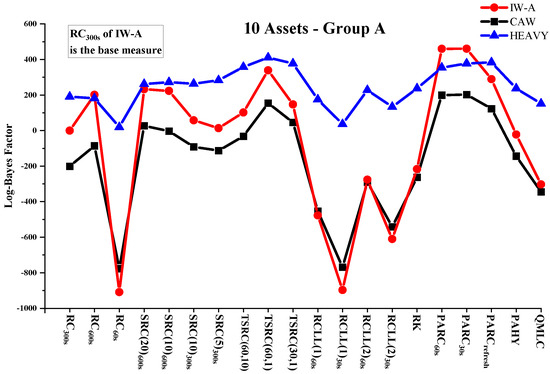
Figure 1. Log Bayes factors (10 assets—Group A).

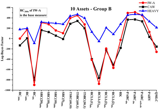
Figure 2. Log Bayes factors (10 assets—Group B).

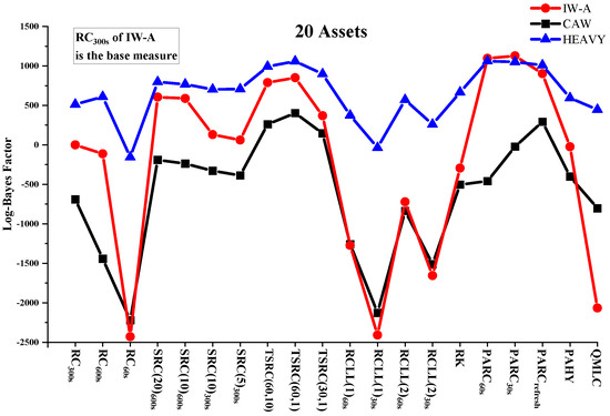
Figure 3. Log Bayes factors (20 assets).

Table 5. Prior sensitivity check.

			Less Sparse Priors		More Sparse Priors
	$\mathit{N}(\mathbf{0},{\mathbf{10}}^{\mathbf{2}})$		$\mathit{N}(\mathbf{0},\mathbf{1})$		$\mathbf{N}(\mathbf{0},{\mathbf{100}}^{\mathbf{2}})$
Estimators	$\mathcal{LPL}$	log-BF	$\mathcal{LPL}$	log-BF	$\mathcal{LPL}$	log-BF
${\mathrm{RC}}_{300s}$	−39,829.0	0	−39,829.3	0	−39,828.8	0
${\mathrm{RC}}_{600s}$	−39,628.1	200.9	−39,626.1	203.2	−39,624.6	204.2
${\mathrm{RC}}_{60s}$	−40,737.5	−908.5	−40,734.6	−905.3	−40,735.6	−906.8
$\mathrm{SRC}{\left(20\right)}_{600s}$	−39,596.2	232.8	−39,588.8	240.5	−39,589.3	239.5
$\mathrm{SRC}{\left(10\right)}_{600s}$	−39,605.6	223.4	−39,600.0	229.3	−39,601.5	227.3
$\mathrm{SRC}{\left(10\right)}_{300s}$	−39,771.2	57.8	−39,771.7	57.6	−39,774.1	54.7
$\mathrm{SRC}{\left(5\right)}_{300s}$	−39,815.7	13.3	−39,823.3	6.0	−39,820.7	8.1
$\mathrm{TSRC}{(60,10)}_{5s}$	−39,727.4	101.6	−39,728.4	100.9	−39,727.9	100.9
$\mathrm{TSRC}{(60,1)}_{5s}$	−39,489.8	339.2	−39,487.0	342.3	−39,487.8	341.0
$\mathrm{TSRC}{(30,1)}_{5s}$	−39,681.7	147.3	−39,684.3	145.0	−39,683.0	145.8
$\mathrm{RCLL}{\left(1\right)}_{60s}$	−40,306.3	−477.3	−40,310.8	−481.5	−40,311.1	−482.3
$\mathrm{RCLL}{\left(1\right)}_{30s}$	−40,726.1	−897.1	−40,723.5	−894.2	−40,721.2	−892.4
$\mathrm{RCLL}{\left(2\right)}_{60s}$	−40,105.7	−276.7	−40,105.6	−276.3	−40,107.4	−278.6
$\mathrm{RCLL}{\left(2\right)}_{30s}$	−40,439.1	−610.1	−40,439.3	−610.0	−40,440.6	−611.8
RK	−40,045.9	−216.9	−40,043.8	−214.5	−40,040.2	−211.4
${\mathrm{PARC}}_{60s}$	−39,369.0	460.0	−39,368.8	460.5	−39,367.7	461.1
${\mathrm{PARC}}_{30s}$	−39,368.6	460.4	−39,368.1	461.2	−39,372.4	456.4
${\mathrm{PARC}}_{\mathrm{refresh}}$	−39,539.9	289.1	−39,539.4	289.9	−39,541.4	287.4
PAHY	−39,851.0	−22.0	−39,852.1	−22.8	−39,850.4	−21.6
QMLC	−40,123.0	−303.0	−40,122.2	−292.9	−40,120.8	−292.0

This table reports the density forecast results based on the IW-A model under three sets of priors.

Figure 4 plots the cumulative log-Bayes factors of several representative estimators (${\mathrm{RC}}_{300s}$, $\mathrm{SRC}{\left(20\right)}_{600s}$, $\mathrm{TSRC}(60,1)$ and ${\mathrm{PARC}}_{\mathrm{refresh}}$) against ${\mathrm{PARC}}_{30s}$ in the three cases according to the IW-A model. The decreasing trend in Figure 4 suggests that the ranking of RCOV estimator is robust in subsample periods.

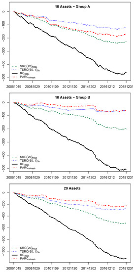
Figure 4. Cumulative log-Bayes factors of ${\mathrm{PARC}}_{30s}$ vs. alternative RC estimators.

The density forecast results confirm several theoretical expectations and findings in the literature. The ranking of TSRC, SRC and RC is consistent with the conclusion in Zhang et al. (2005) that the two-scales estimator has a smaller bias than the subsampled or sparsely-sampled RC. A comparison of SRC estimators confirms that it is better to form a subsampled estimator with low-frequency data and more subsamples. The out-of-sample performance of the RC deteriorates as the sampling frequency increases, which validates the use of low-frequency RC in most empirical studies. The out-of-sample performance of RC and RCLL matches the theoretical results reported by Griffin and Oomen (2011), in which for a fixed sampling frequency, increasing the lead and lag terms reduces the estimation bias. Our results also show that PAHY underperforms PARCs, which is consistent with the finite sample result of PAHY documented by Christensen et al. (2010).

The variation in return density forecasts suggests that the choice of RCOV measure matters greatly with regard to prediction. For example, in the 20 assets application using the IW-A model, switching from ${\mathrm{RC}}_{60s}$ to ${\mathrm{PARC}}_{30s}$ increases the predictive likelihood from −80,200.9 to −76,645.5, a log-Bayes factor of 3555.4. Most RCOV modeling works try to improve the forecasts by adjusting the model specifications and stochastic assumptions, while our results shed light on a different perspective; that is, the choice of RCOV estimator is also important in the pursuit of better predictability.

The density forecast results also show that the comparison of RCOV models could be sensitive to the choice of RCOV. For example, when using ${\mathrm{PARC}}_{30s}$ or ${\mathrm{PARC}}_{60s}$ as the RCOV data, the IW-A model produces the best density forecast results, followed by HEAVY and CAW. In contrast, HEAVY performs better than IW-A for most of the other measures. Among the three joint models, IW-A has the highest sensitivity to RCOV inputs. Taking the 10 assets group A as an example, the log Bayes factor between the best and worst estimators is over 1300 under the IW-A model, while the predictive likelihood ranges under CAW and HEAVY are around 1000 and 400, respectively. Different distributional assumptions and model specifications are potential reasons for the sensitivity difference. In the HEAVY model, the return covariance matrix is estimated conditional on both returns and RCOVs. Therefore, the additional information from returns mitigates poor RCOV measures’ negative influence but diminishes the prediction improvement offered by good RCOV measures. Compared with the IW-A model, the CAW model captures stronger volatility persistence, so its prediction is less sensitive to newly arrived RCOV data. The IW-A and CAW models also differ in RCOV distributional assumptions, which further contributes to the forecasting results differences.

In addition to the one-period ahead density forecasts, we investigate the performance of RCOV measures based on long horizon density forecasts. Table 6 shows 5-period and 10-period ahead log-predictive likelihoods5 under the IW-A model across the three asset groups. Multiple horizon density forecasts provide a similar ranking of the twenty estimators, compared with the results taken from Table 2, Table 3 and Table 4.

Table 6. Predictive likelihoods of returns over long horizons.

	10 Assets—Group A				10 Assets—Group B				20 Assets
Estimators	${\mathcal{LPL}}_5$	log BF	${\mathcal{LPL}}_{10}$	log BF	${\mathcal{LPL}}_5$	log BF	${\mathcal{LPL}}_{10}$	log BF	${\mathcal{LPL}}_5$	log BF	${\mathcal{LPL}}_{10}$	log BF
${\mathrm{RC}}_{\mathrm{300}s}$	−40,448	0	−40,727	0	−42,847	0	−43,105	0	−78,725	0	−79,125	0
${\mathrm{RC}}_{600s}$	−40,099	349 *	−40,287	440 *	−42,531	316	−42,710	395 *	−78,280	445	−78,628	497
${\mathrm{RC}}_{60s}$	−41,621	−1173	−42,003	−1276	−43,961	−1114	−44,294	−1189	−81,783	−3058	−82,465	−3340
$\mathrm{SRC}{\left(20\right)}_{600s}$	−40,192	256 *	−40,416	311 *	−42,570	277	−42,812	293	−78,196	529	−78,546	579
$\mathrm{SRC}{\left(10\right)}_{600s}$	−40,203	245	−40,428	299	−42,587	260	−42,828	277	−78,181	544	−78,529	596 *
$\mathrm{SRC}{\left(10\right)}_{300s}$	−40,485	−37	−40,772	−45	−42,811	36	−43,092	13	−78,905	−180	−79,365	−240
$\mathrm{SRC}{\left(5\right)}_{300s}$	−40,531	−83	−40,823	−96	−42,845	2	−43,127	−22	−78,969	−244	−79,446	−321
$\mathrm{TSRC}{(60,10)}_{5s}$	−40,527	−79	−40,896	−169	−42,507	340 *	−42,746	359 *	−78,077	648 *	−78,457	668 *
$\mathrm{TSRC}{(60,1)}_{5s}$	−40,179	269 *	−40,435	292 *	−42,501	346 *	−42,761	344	−78,124	601 *	−78,532	593
$\mathrm{TSRC}{(30,1)}_{5s}$	−40,467	−19	−40,772	−45	−42,716	131	−42,984	121	−78,781	−56	−79,278	−153
$\mathrm{RCLL}{\left(1\right)}_{60s}$	−41,127	−679	−41,471	−744	−43,433	−586	−43,751	−646	−80,534	−1809	−81,136	−2011
$\mathrm{RCLL}{\left(1\right)}_{30s}$	−41,624	−1176	−42,013	−1286	−43,965	−1118	−44,332	−1227	−81,822	−3097	−82,517	−3392
$\mathrm{RCLL}{\left(2\right)}_{60s}$	−40,881	−443	−41,202	−475	−43,172	−325	−43,471	−366	−79,887	−1162	−80,443	−1318
$\mathrm{RCLL}{\left(2\right)}_{30s}$	−41,304	−856	−41,667	−940	−43,634	−787	−43,983	−878	−81,014	−2289	−81,655	−2530
RK	−40,936	−488	−41,308	−581	−43,073	−226	−43,370	−265	−79,477	−752	−80,011	−886
${\mathrm{PARC}}_{60s}$	−39,868	580 *	−40,024	703 *	−42,286	561 *	−42,491	614 *	−77,479	1246 *	−77,729	1396 *
${\mathrm{PARC}}_{30s}$	−39,925	523 *	−40,117	610 *	−42,324	523 *	−42,543	562 *	−77,576	1149 *	−77,870	1255 *
${\mathrm{PARC}}_{\mathrm{refresh}}$	−40,311	137	−40,592	135	−42,493	354 *	−42,744	361 *	−78,100	625 *	−78,497	628 *
PAHY	−40,763	−315	−41,093	−366	−42,918	−71	−43,203	−98	−79,343	−618	−79,986	−861
QMLC	−40,971	−523	−41,378	−651	−43,553	−706	−43,906	−801	−81,557	−2832	−82,019	−2894

The base RCOV measure for log-BF computation is RC_300s. Bold numbers indicate the highest log-BF values, and the top 5 results are labelled with *.

5.2. Portfolio Allocation

In this section, we evaluate the out-of-sample performance of RCOV estimators from a portfolio optimization perspective. Through forming mean-variance portfolios using predicted covariance, the predictive performance of RCOV estimators can be indirectly assessed based on portfolio performance measures such as standard deviation or Sharpe ratio. Given the predictive covariance ${\mathsf{\Sigma }}_{t+1}$ of next-period returns, the optimal weight $w_{t+1}$ can be obtained by solving the following optimization problem:

$$\min w_{t+1}^{\prime }{\mathsf{\Sigma }}_{t+1}{w}_{t+1},\mathrm{subject}\mathrm{to}{w}_{t+1}^{\prime }\iota =1,$$

(38)

where ${\mathsf{\Sigma }}_{t+1}=\widehat{\mathrm{Cov}}\left(R_{t+1}\right|{\mathcal{F}}_t,\mathcal{M})$. Under IW-A, CAW and HEAVY models, ${\mathsf{\Sigma }}_{t+1}$ are calculated according to Equations (35)–(37). The realized portfolio return $r_{t+1}^p=w_{t+1}^{\prime }{R}_{t+1}$ and the out-of-sample portfolio variance is given as

$${\sigma }_p^2=\frac{1}{T-t_0}\sum _{t=t_0+1}^T{(r_t^p-{\overline{r}}^p)}^2.$$

(39)

The estimator that leads to the smallest ${\sigma }_p^2$ is considered to be the best6.

Table 7 reports the standard deviations of global minimum variance (GMV) portfolios based on the IW-A model7 with various RCOV measures. The comparison results based on portfolio exercises are generally consistent with those obtained from the density forecasts. For example, ${\mathrm{PARC}}_{30s}$, ${\mathrm{PARC}}_{60s}$, TSRC(60,1), and $\mathrm{SRC}{\left(10\right)}_{600s}$ lead to portfolios with relatively low variance. However, the difference among standard deviations of GMV portfolios is marginal. To further investigate whether the difference is significant, we apply the model confidence set (MCS) introduced by Hansen et al. (2011) to obtain a set of estimators that includes the optimal one. Table 7 provides MCS test p-values for each covariance matrix estimator. In the 10-asset group A, estimators excluded are ${\mathrm{RC}}_{60s}$, $\mathrm{SRC}{\left(10\right)}_{300s}$, ${\mathrm{RCLL}\left(2\right)}_{30s}$, ${\mathrm{RCLL}\left(1\right)}_{30s}$, RK, PAHY and QMLC at the 25% significance level. The model confidence set could exclude underperforming RCOV measures, but fails to suggest the optimal one.

Table 7. Standard deviations of global minimum variance portfolio returns (IW-A model).

	10 Assets—A		10 Assets—B		20 Assets
	${\mathbf{\sigma }}_{\mathrm{GMV}}$	${\mathbf{p}}_{\mathrm{MCS}}$	${\mathbf{\sigma }}_{\mathrm{GMV}}$	${\mathbf{p}}_{\mathrm{MCS}}$	${\mathbf{\sigma }}_{\mathrm{GMV}}$	${\mathbf{p}}_{\mathrm{MCS}}$
${\mathrm{RC}}_{300s}$	0.6889	0.363 *	0.8003	0.151	0.6631	0.915 *
${\mathrm{RC}}_{600s}$	0.6850	0.548 *	0.7903	0.875 *	0.6867	0.050
${\mathrm{RC}}_{60s}$	0.7031	0.057	0.8028	0.072	0.6770	0.132
$\mathrm{SRC}{\left(20\right)}_{600s}$	0.6843	0.385 *	0.7922	0.631 *	0.6608	0.960 *
$\mathrm{SRC}{\left(10\right)}_{600s}$	0.6813	0.628 *	0.7914	0.860 *	0.6615	0.929 *
$\mathrm{SRC}{\left(10\right)}_{300s}$	0.6929	0.180	0.7930	0.474 *	0.6626	0.891 *
$\mathrm{SRC}{\left(5\right)}_{300s}$	0.6893	0.383 *	0.7898	0.875 *	0.6616	0.943 *
$\mathrm{TSRC}{(60,10)}_{5s}$	0.6905	0.371 *	0.7892	0.875 *	0.6603	0.960 *
$\mathrm{TSRC}{(60,1)}_{5s}$	0.6881	0.385 *	0.7869	1.000 *	0.6593	0.970 *
$\mathrm{TSRC}{(30,1)}_{5s}$	0.6938	0.298 *	0.7890	0.875 *	0.6662	0.686 *
$\mathrm{RCLL}{\left(1\right)}_{60s}$	0.6962	0.245 *	0.7977	0.112	0.6706	0.431 *
$\mathrm{RCLL}{\left(1\right)}_{30s}$	0.7022	0.106	0.8090	0.013	0.6788	0.172
$\mathrm{RCLL}{\left(2\right)}_{\mathrm{60}s}$	0.6940	0.332 *	0.7931	0.665 *	0.6661	0.792 *
$\mathrm{RCLL}{\left(2\right)}_{30s}$	0.6982	0.186	0.8039	0.041	0.6745	0.226 *
RK	0.6993	0.069	0.7987	0.274 *	0.6704	0.351 *
${\mathrm{PARC}}_{\mathrm{60}s}$	0.6786	1.000 *	0.7911	0.875 *	0.6591	0.970 *
${\mathrm{PARC}}_{\mathrm{30}s}$	0.6805	0.628 *	0.7899	0.875 *	0.6585	1.000 *
${\mathrm{PARC}}_{\mathrm{refresh}}$	0.6907	0.362 *	0.7892	0.875 *	0.6632	0.869 *
PAHY	0.6966	0.095	0.7968	0.194	0.6689	0.276*
QMLC	0.7049	0.077	0.8161	0.022	0.6713	0.580 *

σ_GMV is the standard deviation of global minimum variance portfolio’s returns. p_MCS is the p-value in the model confidence set test. p-values with * indicate the estimator belongs to the best groups at 75% confidence level.

Despite the fact that both the density-forecast and portfolio-based methods are able to eliminate several inferior RCOV estimators, the latter fails to suggest outperforming ones. Compared with the portfolio-based method, the density forecast method is more direct as it ranks RCOV based on density forecasts of multivariate return vectors, rather than univariate portfolio measures. Another drawback of the portfolio-based method is that ranking of covariance estimators is sensitive to the choice of out-of-sample size and significance measurement8.

5.3. Close-to-Close Data

Previous empirical works use open-to-close data, which only account for information during trading hours. To investigate the robustness of our approach, we evaluate RCOV measures based on density forecasts of close-to-close returns. Following Fleming et al. (2003) and de Pooter et al. (2008), the close-to-close covariance matrix is formed by summing intraday covariance and the outer product of overnight returns.

$${\mathrm{RCOV}}_t^{cc}=R_t^{co}{R}_t^{c{o}^{\prime }}+{\mathrm{RCOV}}_t^{oc},$$

(40)

where ${\mathrm{RCOV}}_t^{oc}$ is a realized measure over trading hours and $R_t^{co}$ stands for the overnight log returns, which are formed using the opening price on day t and the closing price on day $t-1$.

Table 8 reports the log-predictive likelihood of close-to-close returns using the HEAVY and CAW models. Even though adding the common overnight covariance component makes the competing covariance estimators more similar, the proposed approach is still sufficiently robust to evaluate estimators, and the rankings remain relatively consistent. ${\mathrm{PARC}}_{30s}$, ${\mathrm{PARC}}_{60s}$, $\mathrm{TSRC}(60,{1)}_{5s}$, $\mathrm{SRC}{\left(20\right)}_{600s}$ and $\mathrm{SRC}{\left(10\right)}_{600s}$ remain the top-performing RCOV measures.

Table 8. Predictive likelihoods of close-to-close return.

	HEAVY Model				CAW Model
	Group A		Group B		Group A		Group B
Estimators	$\mathcal{LPL}$	log BF	$\mathcal{LPL}$	log BF	$\mathcal{LPL}$	log BF	$\mathcal{LPL}$	log BF
${\mathrm{RC}}_{300s}$	−44,011.3	0	−46,244.7	0	−44,793.1	0	−46,941.3	0
${\mathrm{RC}}_{600s}$	−43,993.3	18.0	−46,221.2	23.5	−44,699.1	94.0	−46,852.9	88.4
${\mathrm{RC}}_{60s}$	−44,150.2	−138.9	−46,437.0	−192.3	−45,253.9	−460.8	−47,442.5	−501.2
$\mathrm{SRC}{\left(20\right)}_{600s}$	−43,966.0	45.3	−46,165.9	78.8	−44,706.1	87.0	−46,789.0	152.3
$\mathrm{SRC}{\left(10\right)}_{600s}$	−43,970.9	40.4	−46,170.4	74.3	−44,660.1	133.0	−46,795.7	145.6
$\mathrm{SRC}{\left(10\right)}_{300s}$	−43,972.4	38.9	−46,178.5	66.2	−44,755.3	37.8	−46,875.0	66.3
$\mathrm{SRC}{\left(5\right)}_{300s}$	−43,970.8	40.5	−46,188.0	56.7	−44,746.1	47.0	−46,855.5	85.8
$\mathrm{TSRC}{(60,10)}_{5s}$	−43,952.6	58.7 *	−46,114.8	129.9 *	−44,755.7	37.4	−46,696.7	244.6 *
$\mathrm{TSRC}{(60,1)}_{5s}$	−43,918.9	92.4 *	−46,107.0	137.7 *	−44,578.4	214.7 *	−46,658.9	282.4 *
$\mathrm{TSRC}{(30,1)}_{5s}$	−43,937.1	74.2 *	−46,146.7	98.0	−44,640.9	152.2 *	−46,739.5	201.8
$\mathrm{RCLL}{\left(1\right)}_{60s}$	−44,037.0	−25.7	−46,278.4	−33.7	−44,984.4	−191.3	−47,152.1	−210.8
$\mathrm{RCLL}{\left(1\right)}_{30s}$	−44,141.2	−129.9	−46,419.4	−174.7	−45,225.7	−432.6	−47,408.8	−467.5
$\mathrm{RCLL}{\left(2\right)}_{60s}$	−44,002.9	8.4	−46,232.8	11.9	−44,870.4	−77.3	−47,024.7	−83.4
$\mathrm{RCLL}{\left(2\right)}_{30s}$	−44,071.2	−59.9	−46,314.9	−70.2	−45,076.9	−283.8	−47,215.3	−274.0
RK	−44,014.5	−3.2	−46,199.5	45.2	−44,850.0	−56.9	−46,881.7	59.6
${\mathrm{PARC}}_{60s}$	−43,962.9	48.4	−46,127.4	117.3 *	−44,636.2	156.9 *	−46,654.3	287 *
${\mathrm{PARC}}_{30s}$	−43,953.1	58.2 *	−46,120.6	124.1 *	−44,588.0	205.1 *	−46,650.7	290.6 *
${\mathrm{PARC}}_{\mathrm{refresh}}$	−43,932.8	78.5 *	−46,118.3	126.4 *	−44,609.7	183.4 *	−46,643.8	297.5 *
PAHY	−44,020.5	−9.2	−46,178.3	66.4	−44,780.9	12.2	−46,829.8	111.5
QMLC	−44,096.5	−85.2	−46,247.2	−2.5	−44,925.6	−132.5	−46,951.8	−10.5

This table reports the density forecast of close-to-close returns in the two 10-assets cases. The base RCOV measure for log-BF computation is RC_300s. Bold numbers indicate the highest log-BF values, and the top 5 results are labelled with *.

6. Conclusions

Existing methods of evaluating RCOV estimators empirically rely on portfolio analysis, which compare RCOV measures indirectly using univariate measures such as portfolio standard deviation or Sharpe ratio. The comparison of RCOV measures’ predictive power on return density forecasts is not well investigated in the existing literature. This paper fills the gap by suggesting a density-forecast-based method to evaluate RCOV measures. Given that covariances are not observable, while returns are, the joint modeling of returns and RCOVs enables the evaluation of RCOV estimators via return density forecasts. We test the empirical predictive power of a list of popular RCOV estimators and found several estimators consistently outperform others. The density-forecast-based evaluation method is robust to various RCOV models, datasets, data dimensions and forecast horizons. Another important insight is that the RCOV measures should be carefully selected in covariance modeling, as the choice of RCOV measures can significantly impact a model’s forecasting performance.

Appendix A.1. IW-A Model Estimation Steps

The parameters to be sampled are $\mu ,\nu ,b_1,b_2,b_3,{\ell }_2,{\ell }_3$. We divide them into the following three blocks and iteratively sample them from their conditional posterior distributions.

$$\begin{array}{c}\hfill \begin{array}{cc}1.\hfill & \mu |R_{1:T},{\mathsf{\Sigma }}_{1:T},\hfill \\ 2.\hfill & \nu ,b_1,b_2,b_3|{\ell }_2,{\ell }_3,{\mathsf{\Sigma }}_{1:T},\hfill \\ 3.\hfill & {\ell }_2,{\ell }_3|\nu ,b_1,b_2,b_3,{\mathsf{\Sigma }}_{1:T}.\hfill \end{array}\end{array}$$

$\mu$ is sampled by a Gibbs sampler as its conditional posterior is a multivariate normal:

$$\begin{array}{c}\hfill \mu |R_{1:T},{\mathsf{\Sigma }}_{1:T}\sim N({\overline{m}}_{\mu },{\overline{V}}_{\mu }),\end{array}$$

where ${\overline{V}}_{\mu }={(\frac{1}{100}I+{\sum }_{t=1}^T{\mathsf{\Sigma }}_t^{-1})}^{-1}$ and ${\overline{m}}_{\mu }={\overline{V}}_{\mu }{\sum }_{t=1}^T{\mathsf{\Sigma }}_t^{-1}{R}_t$.

The joint conditional posterior of $\nu ,b_1,b_2,b_3$ is

$$\begin{array}{ccc}\hfill p(\nu ,b_1,b_2,b_3|{\ell }_2,{\ell }_3,{\mathsf{\Sigma }}_{1:T})& \propto & p(\nu ,b_1,b_2,b_3)\prod _{t=1}^{T}IW\left({\mathsf{\Sigma }}_t\right|\nu ,(\nu -d-1)V_t)\hfill \\ & =& p(\nu ,b_1,b_2,b_3)\prod _{t=1}^T\frac{|{\mathsf{\Sigma }}_t{|}^{-\frac{\nu +d+1}{2}}{\left|(\nu -d-1)V_t\right|}^{\frac{\nu }{2}}}{2^{\frac{\nu d}{2}}{\prod }_{j=1}^d\mathsf{\Gamma }\left(\frac{\nu +1-j}{2}\right)}\hfill \\ \hfill & & exp\left(-\frac{1}{2}Tr\left({\mathsf{\Sigma }}_t^{-1}(\nu -d-1)V_t\right)\right).\hfill \end{array}$$

We sample $\nu ,b_1,b_2,b_3$ by applying a Metropolis-Hastings (MH) algorithm with random walk sampler. A multivariate normal serves as the proposal distribution. Given the current values $\{\nu ,b_1,b_2,b_3\}$ in the MCMC chain, the new proposal $\{{\nu }^{{}^{\prime }},b_1^{{}^{\prime }},b_2^{{}^{\prime }},b_3^{{}^{\prime }}\}$ is accepted with probability

$$\begin{array}{c}\hfill min\left\{\frac{p({\nu }^{{}^{\prime }},b_1^{{}^{\prime }},b_2^{{}^{\prime }},b_3^{{}^{\prime }}|{\ell }_2,{\ell }_3,{\mathsf{\Sigma }}_{1:T})}{p(\nu ,b_1,b_2,b_3|{\ell }_2,{\ell }_3,{\mathsf{\Sigma }}_{1:T})},1\right\}.\end{array}$$

The joint conditional posterior of ${\ell }_2,{\ell }_3$ is

$$\begin{array}{ccc}\hfill p({\ell }_2,{\ell }_3|\nu ,b_1,b_2,b_3,{\mathsf{\Sigma }}_{1:T})& \propto & p({\ell }_2,{\ell }_3)\prod _{t=1}^{T}IW\left({\mathsf{\Sigma }}_t\right|\nu ,(\nu -d-1)V_t).\hfill \end{array}$$

${\ell }_2$ and ${\ell }_3$ are sequentially sampled by MH algorithms with the following proposal density:

$$q(\ell )=\frac{{\lambda }^{\ell }{e}^{-\lambda }}{2\ell !}$$

and we set $\lambda =2$. The new proposal $\{{\ell }_2{}^{\prime },{\ell }_3{}^{\prime }\}$ is accepted with probability

$$\begin{array}{c}\hfill min\left\{\frac{p({\ell }_2^{{}^{\prime }},{\ell }_3^{{}^{\prime }},|\nu ,b_1,b_2,b_3,{\mathsf{\Sigma }}_{1:T})}{p({\ell }_2,{\ell }_3|\nu ,b_1,b_2,b_3,{\mathsf{\Sigma }}_{1:T})},1\right\}.\end{array}$$

Appendix A.2. CAW Model Estimation Steps

The parameters set contains $\mu ,\nu ,a_1,a_2,b_1,b_2$, where $a_i$ and $b_i$ are vectors of diagonal elements of $A_i$ and $B_i$, respectively, for $i=1,2$. We iteratively sample the following two blocks of parameters in Bayesian estimation.

$$\begin{array}{c}\hfill \begin{array}{cc}1.\hfill & \mu |R_{1:T},{\mathsf{\Sigma }}_{1:T},\hfill \\ 2.\hfill & \nu ,a_1,a_2,b_1,b_2|{\mathsf{\Sigma }}_{1:T}.\hfill \end{array}\end{array}$$

The same Gibbs step of sampling $\mu$ in the IW-A model estimation is used to sample $\mu$ since the two models share the same conditional posterior of $\mu$. The joint conditional posterior of $\nu ,a_1,a_2,b_1,b_2$ is

$$\begin{array}{ccc}\hfill p(\nu ,a_1,a_2,b_1,b_2|{\mathsf{\Sigma }}_{1:T})& \propto & p(\nu ,a_1,a_2,b_1,b_2)\prod _{t=1}^{T}W\left({\mathsf{\Sigma }}_t\right|\nu ,V_t/\nu )\hfill \\ & =& p(\nu ,a_1,a_2,b_1,b_2)\prod _{t=1}^T\frac{|{\mathsf{\Sigma }}_t{|}^{\frac{\nu -d-1}{2}}{|V_t/\nu |}^{-\frac{\nu }{2}}}{2^{\frac{\nu d}{2}}{\prod }_{j=1}^d\mathsf{\Gamma }\left(\frac{\nu +1-j}{2}\right)}exp\left(-\frac{1}{2}Tr\left({\mathsf{\Sigma }}_t\nu V_t^{-1}\right)\right).\hfill \end{array}$$

We sample $\nu ,a_1,a_2,b_1,b_2$ by applying a MH algorithm with random walk sampler similarly to step 2 in the estimation of the IW-A model. The new proposal $\{{\nu }^{{}^{\prime }},a_1^{{}^{\prime }},a_2^{{}^{\prime }},b_1^{{}^{\prime }},b_2^{{}^{\prime }}\}$ is accepted with probability

$$\begin{array}{c}\hfill min\left\{\frac{p({\nu }^{{}^{\prime }},a_1^{{}^{\prime }},a_2^{{}^{\prime }},b_1^{{}^{\prime }},b_2^{{}^{\prime }}|{\mathsf{\Sigma }}_{1:T})}{p(\nu ,a_1,a_2,b_1,b_2|{\mathsf{\Sigma }}_{1:T})},1\right\}.\end{array}$$

Appendix A.3. HEAVY Model Estimation Steps

The parameter set $\mathsf{\Theta }$ to be sampled includes $\{\nu ,{\nu }_r,a_H,a_V,b_H,b_V\}$, where $a_i$ and $b_i$ are vectors of diagonal elements of $A_i$ and $B_i$, respectively, for $i=H,V$. We sample all the parameters in one block. The joint posterior is

$$\begin{array}{ccc}& & p(\nu ,{\nu }_r,a_H,a_V,b_H,b_V|R_{1:T},{\mathsf{\Sigma }}_{1:T})\hfill \\ & \propto & p(\nu ,{\nu }_r,a_H,a_V,b_H,b_V)\prod _{t=1}^{T}St\left(R_t\right|0,\frac{{\nu }_r-2}{{\nu }_r}{H}_t,{\nu }_r)W\left({\mathsf{\Sigma }}_t\right|\nu ,V_t/\nu )\hfill \\ & =& \prod _{t=1}^T\frac{\mathsf{\Gamma }[({\nu }_r+d)/s]}{\mathsf{\Gamma }({\nu }_r/2){\nu }_r^{d/2}{\pi }^{d/2}{|({\nu }_r-2)/{\nu }_r{H}_t|}^{1/2}}{\left[1+\frac{1}{{\nu }_r-2}{R}_t^{\prime }{H}_t^{-1}{R}_t\right]}^{-\frac{{\nu }_r+2}{2}}\hfill \\ & & ·\frac{|{\mathsf{\Sigma }}_t{|}^{\frac{\nu -d-1}{2}}{|V_t/\nu |}^{-\frac{\nu }{2}}}{2^{\frac{\nu d}{2}}{\prod }_{j=1}^d\mathsf{\Gamma }\left(\frac{\nu +1-j}{2}\right)}exp\left(-\frac{1}{2}Tr\left({\mathsf{\Sigma }}_t\nu V_t^{-1}\right)\right)\hfill \\ & & ·p(\nu ,{\nu }_r,a_H,a_V,b_H,b_V).\hfill \end{array}$$

where $H_t=C_H+B_H{H}_{t-1}{B}_H^{\prime }+A_H{\mathsf{\Sigma }}_{t-1}{A}_H^{\prime }$ and $V_t=C_V+B_V{V}_{t-1}{B}_V^{\prime }+A_V{\mathsf{\Sigma }}_{t-1}{A}_V^{\prime }$. We apply a MH algorithm with random walker proposal to sample $\nu ,{\nu }_r,a_H,a_V,b_H,b_V$. The new proposal $\{{\nu }^{{}^{\prime }},{\nu }_r^{{}^{\prime }},a_H^{{}^{\prime }},a_V^{{}^{\prime }},b_H^{{}^{\prime }},b_V^{{}^{\prime }}\}$ is accepted with probability

$$\begin{array}{c}\hfill min\left\{\frac{p({\nu }^{{}^{\prime }},{\nu }_r^{{}^{\prime }},a_H^{{}^{\prime }},a_V^{{}^{\prime }},b_H^{{}^{\prime }},b_V^{{}^{\prime }}|R_{1:T},{\mathsf{\Sigma }}_{1:T})}{p(\nu ,{\nu }_r,a_H,a_V,b_H,b_V|R_{1:T},{\mathsf{\Sigma }}_{1:T})},1\right\}.\end{array}$$

References

- Aït-Sahalia, Yacine, Jianqing Fan, and Dacheng Xiu. 2010. High-Frequency Covariance Estimates With Noisy and Asynchronous Financial Data. Journal of the American Statistical Association 105: 1504–17. [Google Scholar] [CrossRef]
- Amendola, Alessandra, Manuela Braione, Vincenzo Candila, and Giuseppe Storti. 2020. A model confidence set approach to the combination of multivariate volatility forecasts. International Journal of Forecasting 36: 873–91. [Google Scholar] [CrossRef]
- Andersen, Torben G., Tim Bollerslev, Francis X. Diebold, and Paul Labys. 2003. Modeling and Forecasting Realized Volatility. Econometrica 71: 579–625. [Google Scholar] [CrossRef]
- Asai, Manabu, and Michael McAleer. 2015. Forecasting co-volatilities via factor models with asymmetry and long memoryt in realized covariance. Journal of Econometrics 189: 251–62. [Google Scholar] [CrossRef]
- Aït-Sahalia, Yacine, and Loriano Mancini. 2008. Out of sample forecasts of quadratic variation. Journal of Econometrics 147: 17–33. [Google Scholar] [CrossRef]
- Bannouh, Karim, Dick van Dijk, and Martin Martens. 2009. Range-Based Covariance Estimation Using High-Frequency Data: The Realized Co-Range. Journal of Financial Econometrics 7: 341–72. [Google Scholar] [CrossRef][Green Version]
- Barndorff-Nielsen, Ole E., Peter Reinhard Hansen, Asger Lunde, and Neil Shephard. 2009. Realized kernels in practice: Trades and quotes. Econometrics Journal 12: C1–C32. [Google Scholar] [CrossRef]
- Barndorff-Nielsen, Ole E., Peter Reinhard Hansen, Asger Lunde, and Neil Shephard. 2011. Multivariate realised kernels: Consistent positive semi-definite estimators of the covariation of equity prices with noise and non-synchronous trading. Journal of Econometrics 162: 149–69. [Google Scholar] [CrossRef]
- Barndorff-Nielsen, Ole E., and Neil Shephard. 2004. Econometric analysis of realized covariation: High frequency based covariance, regression, and correlation in financial economics. Econometrica 72: 885–925. [Google Scholar] [CrossRef]
- Bauer, Gregory, and Keith Vorkink. 2011. Forecasting multivriate realized stock market volatility. Journal of Econometrics 160: 79–109. [Google Scholar] [CrossRef]
- Cech, Frantsek, and Jozef Barunik. 2017. On the modelling and forecasting of multivariate realzied volatility: Generalized heterogeneous autoregressive (GHAR) model. Journal of Forecasting 36: 181–206. [Google Scholar] [CrossRef]
- Chiriac, Roxana, and Valeri Voev. 2010. Modelling and forecasting multivariate realized volatility. Journal of Applied Econometrics 26: 922–47. [Google Scholar] [CrossRef]
- Christensen, Kim, Silja Kinnebrock, and Mark Podolskij. 2010. Pre-averaging estimators of the ex-post covariance matrix in noisy diffusion models with non-synchronous data. Journal of Econometrics 159: 116–33. [Google Scholar] [CrossRef]
- Corsi, Fulvio, Stefano Peluso, and Francesco Audrino. 2015. Missing in asynchronicity: A kalman-em approach for multivariate realized covariance estimation. Journal of Applied Econometrics 30: 377–97. [Google Scholar] [CrossRef]
- de Pooter, Michiel, Martin Martens, and Dick van Dijk. 2008. Predicting the daily covariance matrix for s&p 100 stocks using intraday data—But which frequency to use? Econometric Reviews 27: 199–229. [Google Scholar] [CrossRef]
- Dimson, Elroy. 1979. Risk measurement when shares are subject to infrequent trading. Journal of Financial Economics 7: 197–226. [Google Scholar] [CrossRef]
- Fan, Jianqing, Yingying Li, and Ke Yu. 2012. Vast volatility matrix estimation using high-frequency data for portfolio selection. Journal of the American Statistical Association 107: 412–28. [Google Scholar] [CrossRef]
- Fleming, Jeff, Chris Kirby, and Barbara Ostdiek. 2003. The economic value of volatility timing using realized volatility. Journal of Financial Economics 67: 473–509. [Google Scholar] [CrossRef]
- Golosnoy, Vasyl, Bastian Gribisch, and Roman Liesenfeld. 2012. The conditional autoregressive wishart model for multivariate stock market volatility. Journal of Econometrics 167: 211–23. [Google Scholar] [CrossRef]
- Gourieroux, Christian, Joann Jasiak, and Razvan Sufana. 2009. The wishart autoregressive process of multivariate stochastic volatility. Journal of Econometrics 150: 167–81. [Google Scholar] [CrossRef]
- Griffin, Jim E., and Roel C. A. Oomen. 2011. Covariance measurement in the presence of non-synchronous trading and market microstructure noise. Journal of Econometrics 160: 58–68. [Google Scholar] [CrossRef]
- Hansen, Peter, Jeremy Large, and Asger Lunde. 2008. Moving Average-Based Estimators of Integrated Variance. Econometric Reviews 27: 79–111. [Google Scholar] [CrossRef]
- Hansen, Peter R., and Asger Lunde. 2006. Realized variance and market microstructure noise. Journal of Business & Economic Statistics 24: 127–61. [Google Scholar]
- Hansen, Peter R., Asger Lunde, and James M. Nason. 2011. The model confidence set. Econometrica 79: 453–97. [Google Scholar] [CrossRef]
- Hansen, Peter Reinhard, Asger Lunde, and Valeri Voev. 2014. Realized beta GARCH: A multivariate GARCH model with realized measures of volatility. Journal of Applied Econometrics 29: 774–99. [Google Scholar] [CrossRef]
- Hautsch, Nikolaus, Lada M. Kyj, and Roel C. A. Oomen. 2012. A blocking and regularization approach to high-dimensional realized covariance estimation. Journal of Applied Econometrics 27: 625–45. [Google Scholar] [CrossRef]
- Hayashi, Takaki, and Nakahiro Yoshida. 2005. On covariance estimation of non-synchronously observed diffusion processes. Bernoulli 11: 359–79. [Google Scholar] [CrossRef]
- Jacod, Jean, Yingying Li, Per A. Mykland, Mark Podolskij, and Mathias Vetter. 2009. Microstructure noise in the continuous case: The pre-averaging approach. Stochastic Processes and Their Applications 119: 2249–76. [Google Scholar] [CrossRef]
- Jin, Xin, and John Maheu. 2013. Modeling realized covariances and returns. Journal of Financial Econometrics 11: 335–69. [Google Scholar] [CrossRef]
- Jin, Xin, and John Maheu. 2016. Bayesian semiparametric modeling of realized covariance matrices. Journal of Econometrics 192: 19–39. [Google Scholar] [CrossRef]
- Jin, Xin, John Maheu, and Qiao Yang. 2019. Bayesian parametric and semiparametric factor models for large realized covariance matrices. Journal of Applied Econometrics 34: 641–60. [Google Scholar] [CrossRef]
- Lunde, Asger, Neil Shephard, and Kevin Sheppard. 2016. Econometric analysis of vast covariance matrices using composite realized kernels and their application to portfolio choice. Journal of Business & Economic Statistics 34: 504–18. [Google Scholar]
- Noureldin, Diaa, Neil Shephard, and Kevin Sheppard. 2012. Multivariate high-frequency-based volatility (HEAVY) models. Journal of Applied Econometrics 27: 907–33. [Google Scholar] [CrossRef]
- Opschoor, Anne, Pawel Janus, Andre Lucas, and Dick Van Dijk. 2018. New Heavy models for fat-tailed realized covariance and returns. Journal of Business and Economic Statistics 36: 643–57. [Google Scholar] [CrossRef]
- Patton, Andrew, and Kevin Sheppard. 2009. Evaluating volatility and correlation forecasts. Chapter 15. In Handbook of Financial Time Series. Berlin/Heidelberg: Springer, pp. 801–38. [Google Scholar]
- Peluso, Stefano, Fulvio Corsi, and Antonietta Mira. 2015. A bayesian high-frequency estimator of the multivariate covariance of noisy and asynchronous returns. Journal of Financial Econometrics 13: 665–97. [Google Scholar] [CrossRef][Green Version]
- Scholes, Myron, and Joseph Williams. 1977. Estimating betas from nonsynchronous data. Journal of Financial Economics 5: 309–27. [Google Scholar] [CrossRef]
- Shen, Keren, Jianfeng Yao, and Wai Keung Li. 2020. Forecasting high-dimensional realized volatility matyrices using a factor model. Quantitative Finance 20: 1879–87. [Google Scholar] [CrossRef]
- Tao, Minjing, Yazhen Wang, Qiwei Yao, and Jian Zou. 2011. Large volatility matrix inference via combining low-frequency and high-frequency approaches. Journal of the American Statistical Association 106: 1025–40. [Google Scholar] [CrossRef]
- Voev, Valeri, and Asger Lunde. 2007. Integrated Covariance Estimation using High-frequency Data in the Presence of Noise. Journal of Financial Econometrics 5: 68–104. [Google Scholar] [CrossRef]
- Xiu, Dacheng. 2010. Quasi-maximum likelihood estimation of volatility with high frequency data. Journal of Econometrics 159: 235–50. [Google Scholar] [CrossRef]
- Yu, Philip, Wai Keung Li, and Fo Chun Ng. 2017. The generalized conditional autoregressive wishart model for multivariate realized volatility. Journal of Business and Economic Statistics 35: 513–27. [Google Scholar] [CrossRef]
- Zhang, Lan. 2011. Estimating covariation: Epps effect, microstructure noise. Journal of Econometrics 160: 33–47. [Google Scholar] [CrossRef]
- Zhang, Lan, Per A. Mykland, and Yacine Aït-Sahalia. 2005. A tale of two time scales: Determining integrated volatility with noisy high-frequency data. Journal of the American Statistical Association 100: 1394–11. [Google Scholar] [CrossRef]
Publisher’s Note: MDPI stays neutral with regard to jurisdictional claims in published maps and institutional affiliations. |
© 2021 by the authors. Licensee MDPI, Basel, Switzerland. This article is an open access article distributed under the terms and conditions of the Creative Commons Attribution (CC BY) license (https://creativecommons.org/licenses/by/4.0/).