Indirect Inference Estimation of Spatial Autoregressions

Abstract

The ordinary least squares (OLS) estimator for spatial autoregressions may be consistent as pointed out by Lee (2002), provided that each spatial unit is influenced aggregately by a significant portion of the total units. This paper presents a unified asymptotic distribution result of the properly recentered OLS estimator and proposes a new estimator that is based on the indirect inference (II) procedure. The resulting estimator can always be used regardless of the degree of aggregate influence on each spatial unit from other units and is consistent and asymptotically normal. The new estimator does not rely on distributional assumptions and is robust to unknown heteroscedasticity. Its good finite-sample performance, in comparison with existing estimators that are also robust to heteroscedasticity, is demonstrated by a Monte Carlo study.

1. Introduction

Spatial autoregressions (SAR) have attracted lots of attention from both practical and theoretical sides in economics and other disciplines of social sciences since the classical work of Cliff and Ord (1981). Its popularity is mainly due to its parsimonious representation of the cross-sectional correlation by a weight matrix. Correlation in spatial data arises naturally due to competition, copycatting, spillover, aggregation, to name just a few. In these contexts, space embodied in the weight matrix can be defined in terms of not only geographical distance but also economic distance.

The spatial autoregression model extends autocorrelation in time series to the spatial dimension in the sense that in the structural equation a spatially “lagged” dependent variable is included as a regressor. In time series, the autoregression model can be estimated consistently by the ordinary least squares (OLS), but for the spatial autoregression, the OLS is usually regarded as an inconsistent method. Robinson (2008) provided an excellent discussion of the intuition behind this. Estimation strategies like the maximum likelihood (ML), quasi maximum likelihood (QML), instrument variables (IV), and generalized method of moments (GMM) have been proposed in the literature. The ML is the most efficient, but it imposes stringent distributional assumptions on the data generating process, whereas both the ML and QML rule out heteroscedasticity in the error term. Further, the (Q)ML method involves calculating the determinant or eigenvalues of a matrix that is of the same size as the sample, and thus many researchers dismiss its use in moderately large samples and advocate the more flexible IV and GMM estimators that may incur less computational burden and are also robust to heteroscedasticity.

Lee (2002) overturned the traditional wisdom regarding the OLS estimator in spatial autoregressions when there are exogenous regressors included. He showed that while the OLS estimator is inconsistent for spatial autoregressions with a sparse weight matrix, it can be consistent when spatial units may have small spatial impacts on other units but each unit may be influenced aggregately by a significant portion of the total units. For the special case of the so-called pure SAR model, namely, when there is no other exogenous regressor, Lee (2002) demonstrated that regardless of the structure of the weight matrix, the OLS estimator is always inconsistent.

In practice, one may have limited knowledge to judge whether a spatial unit is influenced by a significant portion of the total units. When a researcher is constructing the weight matrix, she may know the number of neighboring units for each unit, but she may be unable to tell whether the number of neighbors is significant in finite samples. Thus, this poses a challenge for practitioners regarding the usefulness of the OLS estimator: it may or may not be consistent, depending on the degree of aggregate influence on each unit from other units, which may hardly manifest itself in finite samples. This paper carefully analyzes the asymptotic distribution theory for the OLS estimator. A unified asymptotic distribution result for the recentered OLS estimator is presented under different regimes for the spatial weight matrix. Given the asymptotic result for the recentered OLS estimator, a new estimator based on the indirect inference (II) procedure is proposed.

Kyriacou et al. (2017) novelly used the II procedure to correct the inconsistency of the OLS estimator in the pure SAR model under homoscedasticity. Even though they provided promising simulation results under some mild heteroscedasticity, they have yet to show rigorously how to construct a consistent estimator with no restrictions on the form of heteroscedasticity. In contrast, this paper considers the SAR model with exogenous regressors and it adds to the existing spatial literature with unknown heteroscedasticity.1

Note that the problem of inconsistency (of the OLS estimator) is solely due to the presence of the endogenous spatially lagged variable. Once the spatial autoregression parameter is estimated consistently, the OLS procedure can be used to estimate the remaining parameters, though the asymptotic variance needs to be modified accordingly to take into account the uncertainty in the estimated spatial autoregression parameter.

The structure of this paper is as follows. In the next section, the asymptotic behavior of the OLS estimator is discussed under different spatial scenarios. The II estimator, which aims to correct the possible inconsistency of the OLS estimator, is defined and its asymptotic distribution is derived. A very important message from this section is that regardless of the degree of aggregate influence on each spatial unit from other units, the II procedure can always be used and the resulting estimator is consistent and asymptotically normal. Section 3 discusses the special case of pure SAR. Section 4 provides Monte Carlo evidence of the effectiveness of the II estimation strategy. It shows that the II estimator possesses good finite-sample performance relative to other consistent estimators that are also robust to unknown heteroscedasticity and that the II method may be favored for the purpose of hypothesis testing, especially for testing the spatial autoregression parameter. Section 5 concludes. Some useful lemmas are collected in Appendix A and proofs of the results presented in Section 2 and Section 3 are given in Appendix B.

Throughout this paper, K is used to denote a positive constant on different occasions, arbitrarily large but bounded, that does not depend on the sample size n and whose value may vary in different contexts. ${\mathit{I}}_n$ is the identity matrix of dimension n and ${\mathbf{1}}_n$ is an $n\times 1$ vector of ones. For an $n\times 1$ vector ${\mathit{a}}_n$, $a_{i,n}$ denotes its i-th element and for an $n\times n$ matrix ${\mathit{A}}_n$, $a_{ij,n}$ denotes its $ij$-th element. ${\left|\left|{\mathit{A}}_n\right|\right|}_{\infty }={max}_{1\le i<n}{\sum }_{j=1}^n\left|a_{ij,n}\right|$ and ${\left|\left|{\mathit{A}}_n\right|\right|}_1={max}_{1\le j<n}{\sum }_{i=1}^n\left|a_{ij,n}\right|$ are the maximum row sum norm and maximum column sum norm, respectively. A sequence of matrices $\left\{{\mathit{A}}_n\right\}$ is uniformly bounded in row sum if ${\left|\left|{\mathit{A}}_n\right|\right|}_{\infty }\le K$, and is uniformly bounded in column sum if ${\left|\left|{\mathit{A}}_n\right|\right|}_1\le K$. $\mathrm{tr}$ and ⊙ are matrix trace and Hadamard product operators, respectively. $\mathrm{Dg}\left({\mathit{a}}_n\right)$ denotes a square diagonal matrix with the vector ${\mathit{a}}_n$ spanning the main diagonal, $\mathrm{dg}\left({\mathit{A}}_n\right)$ is an $n\times 1$ column vector that collects in order the diagonal elements of the square matrix ${\mathit{A}}_n$, and $\mathrm{Dg}\left({\mathit{A}}_n\right)=\mathrm{Dg}\left(\mathrm{dg}\left({\mathit{A}}_n\right)\right)$. The subscript 0 is used to signify the true parameter value.

2. Main Results

Consider the SAR model

$${\mathit{y}}_n=\lambda {\mathit{W}}_n{\mathit{y}}_n+{\mathit{X}}_n\mathit{\beta }+{\mathit{u}}_n={\mathit{Z}}_n\mathit{\theta }+{\mathit{u}}_n,$$

(1)

where n is the total number of cross-sectional units, ${\mathit{Z}}_n=({\mathit{W}}_n{\mathit{y}}_n,{\mathit{X}}_n)$, $\mathit{\theta }={(\lambda ,{\mathit{\beta }}^{\prime })}^{\prime }$, ${\mathit{y}}_n$ is an $n\times 1$ vector, collecting observations on the dependent variable, ${\mathit{X}}_n$ is an $n\times k$ matrix of observations on k exogenous nonstochastic regressors with coefficient vector $\mathit{\beta }$, ${\mathit{W}}_n$ is an $n\times n$ matrix of spatial weights with zero diagonals, $\lambda$ is the spatial autoregression coefficient, and ${\mathit{u}}_n$ is an n-dimensional vector of error terms.

For the ease of presentation, the following matrix notation is introduced in this paper:

$$\begin{array}{ll}\hfill & {\mathit{S}}_n\left(\lambda \right)={\mathit{I}}_n-\lambda {\mathit{W}}_n,{\mathit{G}}_n\left(\lambda \right)={\mathit{W}}_n{\mathit{S}}_n^{-1}\left(\lambda \right),{\mathit{M}}_n={\mathit{I}}_n-{\mathit{X}}_n{\left({\mathit{X}}_n^{\prime }{\mathit{X}}_n\right)}^{-1}{\mathit{X}}_n^{\prime },\hfill \\ \hfill & {\mathit{D}}_n\left(\lambda \right)=\mathrm{Dg}\left({\mathit{M}}_n{\mathit{G}}_n\left(\lambda \right)\right),{\mathit{E}}_n\left(\lambda \right)={\mathit{M}}_n{\mathit{G}}_n\left(\lambda \right)-{\mathit{D}}_n\left(\lambda \right).\hfill \end{array}$$

(2)

When a matrix is presented without its argument $\lambda$, it means that it is evaluated at the parameter value ${\lambda }_0$. Namely, ${\mathit{S}}_n={\mathit{S}}_n\left({\lambda }_0\right)$, ${\mathit{G}}_n={\mathit{G}}_n\left({\lambda }_0\right)$, ${\mathit{D}}_n={\mathit{D}}_n\left({\lambda }_0\right)$, and ${\mathit{E}}_n={\mathit{E}}_n\left({\lambda }_0\right)$.

If $\lambda$ is known (equal to its true value), the model becomes a standard linear model with ${\mathit{S}}_n{\mathit{y}}_n$ being the dependent variable; otherwise, ${\mathit{W}}_n{\mathit{y}}_n$ appears on the right-hand side of (1) as a spatially lagged or weighted variable. The OLS estimator of ${\mathit{\theta }}_0$ is ${\widehat{\mathit{\theta }}}_n={\left({\mathit{Z}}_n^{\prime }{\mathit{Z}}_n\right)}^{-1}{\mathit{Z}}_n^{\prime }{\mathit{y}}_n$, which may be inconsistent. Since the inconsistency of ${\widehat{\mathit{\theta }}}_n$ is solely due to the endogenous ${\mathit{W}}_n{\mathit{y}}_n$, the properties of ${\widehat{\lambda }}_n$ (the first element of ${\widehat{\mathit{\theta }}}_n$) are discussed first in this paper. Once a consistent estimator of ${\lambda }_0$ is available, one can show that a consistent estimator of ${\mathit{\beta }}_0$ follows immediately (see Theorem 4 to be introduced).2

Let $r_n=r_{1n}+r_{2n}$, $r_{1n}={\mathit{u}}_n^{\prime }{\mathit{M}}_n{\mathit{G}}_n{\mathit{u}}_n$, $r_{2n}={\mathit{\beta }}_0^{\prime }{\mathit{X}}_n^{\prime }{\mathit{G}}_n^{\prime }{\mathit{M}}_n{\mathit{u}}_n$, $d_n=d_{1n}+d_{2n}+d_{3n}$, $d_{1n}={\mathit{u}}_n^{\prime }{\mathit{G}}_n^{\prime }{\mathit{M}}_n{\mathit{G}}_n{\mathit{u}}_n$, $d_{2n}=2{\mathit{\beta }}_0^{\prime }{\mathit{X}}_n^{\prime }{\mathit{G}}_n^{\prime }{\mathit{M}}_n{\mathit{G}}_n{\mathit{u}}_n$, and $d_{3n}={\mathit{\beta }}_0^{\prime }{\mathit{X}}_n^{\prime }{\mathit{G}}_n^{\prime }{\mathit{M}}_n{\mathit{G}}_n{\mathit{X}}_n{\mathit{\beta }}_0$. By using the partitioned regression formula and substituting ${\mathit{W}}_n{\mathit{y}}_n={\mathit{G}}_n{\mathit{X}}_n{\mathit{\beta }}_0+{\mathit{G}}_n{\mathit{u}}_n$, one may put

$${\widehat{\lambda }}_n-{\lambda }_0=\frac{{\mathit{y}}_n^{\prime }{\mathit{W}}_n^{\prime }{\mathit{M}}_n{\mathit{u}}_n}{{\mathit{y}}_n^{\prime }{\mathit{W}}_n^{\prime }{\mathit{M}}_n{\mathit{W}}_n{\mathit{y}}_n}=\frac{r_n}{d_n}=\frac{r_{1n}+r_{2n}}{d_{1n}+d_{2n}+d_{3n}}.$$

(3)

The following assumptions are made throughout this paper.

Assumption 1.

(i) $\forall i\ne j$, $w_{ij,n}=O\left(h_n^{-1}\right)$, where the rate sequence $\left\{h_n\right\}$ is uniformly bounded away from zero and $\underset{n\to \infty }{lim}{h}_n/n=0$; (ii) the sequence $\left\{{\mathit{W}}_n\right\}$ is is uniformly bounded in row and column sums; (iii) $w_{ii,n}=0$.

Assumption 2.

(i) ${\mathit{S}}_n^{-1}$ exists; (ii) the sequence $\left\{{\mathit{S}}_n^{-1}\right\}$ is uniformly bounded in row and column sums.

Assumption 3.

The error terms $\left\{u_{i,n}\right\}$ in ${\mathit{u}}_n={(u_{1,n},\cdots ,u_{n,n})}^{\prime }$ have following properties: (i) $\mathrm{E}\left(u_{i,n}\right)=0$; (ii) $\mathrm{E}\left(\right|u_{i,n}{|}^{4+\delta })<\infty$ for some positive constant δ; (iii) $u_{i,n}$ and $u_{j,n}$ are independent for any $i\ne j$.

Assumption 4.

${\lambda }_0$ is contained in a compact parameter space Λ. For any admissible $\lambda \in \mathsf{\Lambda }$, $\left\{{\mathit{S}}_n^{-1}\left(\lambda \right)\right\}$ is uniformly bounded in row and column sums.

Assumption 5.

(i) The elements of ${\mathit{X}}_n$ are uniformly bounded constants for all n; (ii) the probability limit Γ of $n^{-1}{\mathit{Z}}_n^{\prime }{\mathit{Z}}_n$ exists and is nonsingular.

Assumption 6.

(i) ${lim}_{n\to \infty }{n}^{-1}\mathrm{Var}\left(r_n\right)$ exists and is nonzero; (ii) ${lim}_{n\to \infty }{n}^{-1}\mathrm{Var}({\mathit{u}}_n^{\prime }{\mathit{E}}_n{\mathit{u}}_n+{\mathit{\beta }}_0^{\prime }{\mathit{X}}_n^{\prime }{\mathit{G}}_n^{\prime }{\mathit{M}}_n{\mathit{u}}_n)$ exists and is nonzero.

Intuitions and related discussions for Assumptions 1–5 are provided in Kelejian and Prucha (2010) and Lee (2001, 2002, 2004). Assumption 1(i) follows naturally when ${\mathit{W}}_n$ is row- or column-normalized, as is typically the case. Assumption 1(ii) and Assumption 2 limit the degree of dependency among the spatial units and is originated by Kelejian and Prucha (1999). Given Assumption 2, the equilibrium solution of ${\mathit{y}}_n$ is ${\mathit{y}}_n={\mathit{S}}_n^{-1}{\mathit{X}}_n{\mathit{\beta }}_0+{\mathit{S}}_n^{-1}{\mathit{u}}_n$. Under Assumption 3, let ${\sigma }_{i,n}^2=\mathrm{E}\left(u_{i,n}^2\right)$, ${\mathsf{\Sigma }}_n=\mathrm{Dg}({\sigma }_{1,n}^2,\cdots ,{\sigma }_{n,n}^2)$, and ${\mathsf{\Sigma }}_n^{\left(j\right)}=\mathrm{Dg}({\mu }_{1,n}^{\left(j\right)},\cdots ,{\mu }_{n,n}^{\left(j\right)})$ with ${\mu }_{i,n}^{\left(j\right)}=\mathrm{E}\left(u_{i,n}^j\right)$, $j=3,4$. Lee (2002) emphasized that Assumption 5(ii) is related to an identification condition for estimation in the least squares and IV frameworks. It rules out possible multicollinearities among ${\mathit{X}}_n$ and ${\mathit{G}}_n{\mathit{X}}_n{\mathit{\beta }}_0$ for large n and implies that the limit of $d_{3n}/n$ is bounded away from zero.3 Assumption 6 ensures that the asymptotic variances of the (properly recentered) OLS estimator and the resulting II estimator are positive.4

2.1. The Asymptotic Behavior of the OLS estimator

From Lemma A6 in Appendix A, $r_{1n}$ and $d_{1n}$ are both $O_P(n/h_n)$, $r_{2n}$ and $d_{2n}$ are both $O_P\left(\sqrt{n}\right)$, and $d_{3n}=O\left(n\right)$. The asymptotic properties of the OLS estimator crucially depend on the magnitude of $h_n$.

When $h_n$ is bounded, the OLS estimator cannot be consistent, since now

$${\widehat{\lambda }}_n-{\lambda }_0=\frac{\frac{1}{n}{r}_{1n}}{\frac{1}{n}{d}_{1n}+\frac{1}{n}{d}_{3n}}+o_P\left(1\right),$$

but the probability limit of the numerator $n^{-1}{r}_{1n}$ is typically nonzero.

If $h_n\to \infty$, $d_{3n}$ dominates the denominator in (3), then

$${\widehat{\lambda }}_n-{\lambda }_0=\frac{\frac{1}{h_n}\left(\frac{h_n}{n}{r}_{1n}\right)+\frac{1}{\sqrt{n}}\left(\frac{1}{\sqrt{n}}{r}_{2n}\right)}{\frac{1}{n}{d}_{3n}}+o_P\left(1\right)\stackrel{p}{\to }0,$$

indicating that ${\widehat{\lambda }}_n$ is consistent as long as $h_n\to \infty$.

More interestingly, the behavior of ${\widehat{\lambda }}_n$ depends on how fast $h_n$ diverges to infinity. If $h_n$ tends to infinity at a rate slower than $\sqrt{n}$, then $r_{1n}$ dominates $r_{2n}$ in the numerator, and

$$h_n({\widehat{\lambda }}_n-{\lambda }_0)=\frac{\frac{h_n}{n}{r}_{1n}}{\frac{1}{n}{d}_{3n}}+o_P\left(1\right),$$

(4)

which implies that ${\widehat{\lambda }}_n$ converges at the slower rate $h_n$, but it does not converge to ${\lambda }_0$ at rate $h_n$, as $\underset{n\to \infty }{plim}(h_n/n)r_{1n}=\underset{n\to \infty }{lim}(h_n/n)\mathrm{tr}\left({\mathsf{\Sigma }}_n{\mathit{M}}_n{\mathit{G}}_n\right)$ is typically nonzero.

If $h_n=O\left(\sqrt{n}\right)$, $r_{1n}$ and $r_{2n}$ are of the same order in the numerator, so

$$\sqrt{n}({\widehat{\lambda }}_n-{\lambda }_0)=\frac{\frac{1}{\sqrt{n}}{r}_{1n}+\frac{1}{\sqrt{n}}{r}_{2n}}{\frac{1}{n}{d}_{3n}}+o_P\left(1\right),$$

(5)

indicating that ${\widehat{\lambda }}_n$ converges at rate $\sqrt{n}$, but at this rate it does not converge to ${\lambda }_0$, as in general $\underset{n\to \infty }{plim}{n}^{-1/2}{r}_{1n}=\underset{n\to \infty }{lim}{n}^{-1/2}\mathrm{tr}\left({\mathsf{\Sigma }}_n{\mathit{M}}_n{\mathit{G}}_n\right)$ is nonzero.

If $h_n$ tends to infinity at a rate faster than $\sqrt{n}$ (and yet smaller than n), namely, $\underset{n\to \infty }{lim}\sqrt{n}/h_n=0$ (and $\underset{n\to \infty }{lim}{h}_n/n=0)$, then in the numerator $r_{2n}$ dominates $r_{1n}$,

$$\sqrt{n}({\widehat{\lambda }}_n-{\lambda }_0)=\frac{\frac{1}{\sqrt{n}}{r}_{2n}}{\frac{1}{n}{d}_{3n}}+o_P\left(1\right),$$

(6)

indicating that ${\widehat{\lambda }}_n$ converges to ${\lambda }_0$ at rate $\sqrt{n}$ and is asymptotically normal if one applies a central limit theorem to $n^{-1/2}{r}_{2n}$.

One sees that the asymptotic behavior of ${\widehat{\lambda }}_n$ depends on the magnitude of $h_n$, which may be unknown in practice. The following theorem shows that if one can properly recenter ${\widehat{\lambda }}_n$, then a unified asymptotic distribution result follows.

Theorem 1.

Under Assumptions 1–6, the OLS estimator ${\widehat{\lambda }}_n$ of ${\lambda }_0$ in the SAR model (1) has the following asymptotic distribution,

$$\sqrt{n}\left({\widehat{\lambda }}_n-{\lambda }_0-\frac{\mathrm{tr}\left({\mathsf{\Sigma }}_n{\mathit{M}}_n{\mathit{G}}_n\right)}{{\mathit{y}}_n^{\prime }{\mathit{W}}_n^{\prime }{\mathit{M}}_n{\mathit{W}}_n{\mathit{y}}_n}\right)\stackrel{d}{\to }\mathrm{N}(0,v),$$

(7)

where

$$v=\underset{n\to \infty }{lim}\frac{n\mathrm{Var}\left(r_n\right)}{{[\mathrm{tr}\left({\mathsf{\Sigma }}_n{\mathit{G}}_n^{\prime }{\mathit{M}}_n{\mathit{G}}_n\right)+{\mathit{\beta }}_0^{\prime }{\mathit{X}}_n^{\prime }{\mathit{G}}_n^{\prime }{\mathit{M}}_n{\mathit{G}}_n{\mathit{X}}_n{\mathit{\beta }}_0]}^2}$$

with

$$\begin{array}{cc}\hfill \mathrm{Var}\left(r_n\right)& =\mathrm{tr}({\mathsf{\Sigma }}_n^{\left(4\right)}\odot {\mathit{M}}_n{\mathit{G}}_n\odot {\mathit{M}}_n{\mathit{G}}_n)+\mathrm{tr}\left[{\mathsf{\Sigma }}_n{\mathit{M}}_n{\mathit{G}}_n{\mathsf{\Sigma }}_n({\mathit{M}}_n{\mathit{G}}_n+{\mathit{G}}_n^{\prime }{\mathit{M}}_n)\right]\hfill \\ \hfill & +{\mathit{\beta }}_0^{\prime }{\mathit{X}}_n^{\prime }{\mathit{G}}_n^{\prime }{\mathit{M}}_n{\mathsf{\Sigma }}_n{\mathit{M}}_n{\mathit{G}}_n{\mathit{X}}_n{\mathit{\beta }}_0+2{\mathit{\beta }}_0^{\prime }{\mathit{X}}_n^{\prime }{\mathit{G}}_n^{\prime }{\mathit{M}}_n\mathrm{dg}({\mathsf{\Sigma }}_n^{\left(3\right)}\odot {\mathit{M}}_n{\mathit{G}}_n).\hfill \end{array}$$

Remark 1.

The recentering term $\mathrm{tr}\left({\mathsf{\Sigma }}_n{\mathit{M}}_n{\mathit{G}}_n\right)/{\mathit{y}}_n^{\prime }{\mathit{W}}_n^{\prime }{\mathit{M}}_n{\mathit{W}}_n{\mathit{y}}_n$ is in fact $\mathrm{E}\left(r_n\right)/d_n$. One could have recentered ${\widehat{\lambda }}_n-{\lambda }_0$ by $\mathrm{E}\left(r_n\right)/\mathrm{E}\left(d_n\right)$. (This is the approach taken by Kyriacou et al. (2017) when dealing with the special case of pure SAR model.) But then by following a similar expansion as in the proof of Theorem 1 (see Appendix B.1), one can find that the asymptotic variance of the resulting recentered estimator is much more complicated, involving the variances of $r_n$ and $d_n$ as well as their covariance.

Remark 2.

When $\underset{n\to \infty }{lim}\sqrt{n}/h_n=0$, the recentering term $\mathrm{tr}\left({\mathsf{\Sigma }}_n{\mathit{M}}_n{\mathit{G}}_n\right)/{\mathit{y}}_n^{\prime }{\mathit{W}}_n^{\prime }{\mathit{M}}_n{\mathit{W}}_n{\mathit{y}}_n$ is in fact $o_P\left(n^{-1/2}\right)$ and the asymptotic distribution of $\sqrt{n}({\widehat{\lambda }}_n-{\lambda }_0)$ centers at zero, so one does not need to recenter ${\widehat{\lambda }}_n-{\lambda }_0$ by $\mathrm{tr}\left({\mathsf{\Sigma }}_n{\mathit{M}}_n{\mathit{G}}_n\right)/{\mathit{y}}_n^{\prime }{\mathit{W}}_n^{\prime }{\mathit{M}}_n{\mathit{W}}_n{\mathit{y}}_n$; nor does one need to recenter it by ${\mathit{y}}_n^{\prime }{\mathit{S}}_n^{\prime }{\mathit{M}}_n{\mathit{D}}_n{\mathit{M}}_n{\mathit{S}}_n{\mathit{y}}_n/{\mathit{y}}_n^{\prime }{\mathit{W}}_n^{\prime }{\mathit{M}}_n{\mathit{W}}_n{\mathit{y}}_n$, which is also $o_P\left(n^{-1/2}\right),$ as in Theorem 2 to be introduced.

Remark 3.

When $h_n$ diverges, one may single out dominating terms in $\mathrm{Var}\left(r_n\right)$ and $\mathrm{E}\left(d_n\right)$ so that a finer expression of $v={lim}_{n\to \infty }[\mathrm{Var}\left(r_n\right)/n]/{[\mathrm{E}\left(d_n\right)/n]}^2$ can be presented. For example, under divergent $h_n$, one can replace $\mathrm{Var}\left(r_n\right)$ with $\mathrm{Var}\left(r_{2n}\right)={\mathit{\beta }}_0^{\prime }{\mathit{X}}_n^{\prime }{\mathit{G}}_n^{\prime }{\mathit{M}}_n{\mathsf{\Sigma }}_n{\mathit{M}}_n{\mathit{G}}_n{\mathit{X}}_n{\mathit{\beta }}_0$ and replace $\mathrm{E}\left(d_n\right)$ with its dominating term ${\mathit{\beta }}_0^{\prime }{\mathit{X}}_n^{\prime }{\mathit{G}}_n^{\prime }{\mathit{M}}_n{\mathit{G}}_n{\mathit{X}}_n{\mathit{\beta }}_0$. When $h_n$ is bounded, however, such replacements are not available and one needs to keep all the term in $\mathrm{Var}\left(r_n\right)$ and $\mathrm{E}\left(d_n\right)$. Moreover, since $\mathrm{Var}\left(r_n\right)$ depends on higher-order moments of u, namely, ${\mathsf{\Sigma }}_n^{\left(3\right)}$ and ${\mathsf{\Sigma }}_n^{\left(4\right)}$, then, with bounded $h_n$, the asymptotic variance v of the recentered OLS estimator depends on them, too.

Remark 4.

In view of Remark 3, under divergent $h_n$, if further ${\mathsf{\Sigma }}_n={\sigma }_0^2{\mathit{I}}_n$, namely, under homoscedasticity with ${\sigma }_0^2=\mathrm{E}\left(u_{i,n}^2\right)$, then v corresponds to the top left element of ${\sigma }_0^2{\mathsf{\Gamma }}^{-1}$. This, together with Remark 2, is in line with the observation in Lee (2002) that the (consistent, uncentered) OLS estimator (when $\underset{n\to \infty }{lim}\sqrt{n}/h_n=0$) has the same limiting distribution of the optimal IV estimator and under normality it has the same limiting distribution of the ML estimator. It also implies that under other cases of divergent $h_n$ (slower than or equal to rate $\sqrt{n}$), as long as the OLS estimator is properly recentered, it achieves the same limiting distribution.

Remark 5.

Theorem 1 gives a unified representation of the asymptotic distribution of the properly recentered OLS estimator, regardless of the possibly unknown magnitude of $h_n$. Further, it facilitates the construction of the indirect inference estimator to be introduced that corrects the inconsistency, when present, of the OLS estimator.

2.2. The Indirect Inference Estimator

One can see from Theorem 1 in the previous subsection that the OLS estimator ${\widehat{\lambda }}_n$ may have an asymptotic bias. Yet a direct feasible bias-correction procedure is not possible, since the bias itself depends on unknown parameters, including ${\lambda }_0$, which may not be consistently estimated by the OLS estimator ${\widehat{\lambda }}_n$. Following Phillips (2012) and Kyriacou et al. (2017), one may define the binding function that involves the bias of ${\widehat{\lambda }}_n$. Unfortunately, the resulting binding function then involves the unknown ${\mathsf{\Sigma }}_n$, which appears in the recentering quantity for the OLS estimator in (7). The strategy in this paper is to replace $\mathrm{tr}\left({\mathsf{\Sigma }}_n{\mathit{M}}_n{\mathit{G}}_n\right)=\mathrm{E}\left({\mathit{u}}_n^{\prime }{\mathit{M}}_n{\mathit{G}}_n{\mathit{u}}_n\right)$ with a term that is of the same order of ${\mathit{u}}_n^{\prime }{\mathit{M}}_n{\mathit{G}}_n{\mathit{u}}_n$ and at the same time does not directly involve ${\mathsf{\Sigma }}_n$.

Recall that ${\mathit{D}}_n=\mathrm{Dg}\left({\mathit{M}}_n{\mathit{G}}_n\right)$. Then under a general form of unknown heteroscedasticity, $\mathrm{tr}\left({\mathsf{\Sigma }}_n{\mathit{M}}_n{\mathit{G}}_n\right)=\mathrm{tr}\left({\mathsf{\Sigma }}_n{\mathit{D}}_n\right)=\mathrm{E}\left({\mathit{u}}_n^{\prime }{\mathit{D}}_n{\mathit{u}}_n\right)$, where ${\mathit{u}}_n={\mathit{S}}_n{\mathit{y}}_n-{\mathit{X}}_n{\mathit{\beta }}_0$. If ${\lambda }_0$ is known, then ${\mathit{\beta }}_0$ can be consistently estimated by ${\tilde{\mathit{\beta }}}_n={\tilde{\mathit{\beta }}}_n\left({\lambda }_0\right)={\left({\mathit{X}}_n^{\prime }{\mathit{X}}_n\right)}^{-1}{\mathit{X}}_n^{\prime }{\mathit{S}}_n{\mathit{y}}_n$. Let ${\tilde{\mathit{u}}}_n={\tilde{\mathit{u}}}_n\left({\lambda }_0\right)={\mathit{S}}_n{\mathit{y}}_n-{\mathit{X}}_n{\tilde{\mathit{\beta }}}_n={\mathit{M}}_n{\mathit{S}}_n{\mathit{y}}_n$. Now one may be able to replace $\mathrm{E}\left({\mathit{u}}_n^{\prime }{\mathit{D}}_n{\mathit{u}}_n\right)$ with ${\tilde{\mathit{u}}}_n^{\prime }{\mathit{D}}_n{\tilde{\mathit{u}}}_n={\mathit{y}}_n^{\prime }{\mathit{S}}_n^{\prime }{\mathit{M}}_n{\mathit{D}}_n{\mathit{M}}_n{\mathit{S}}_n{\mathit{y}}_n$ and use ${\mathit{y}}_n^{\prime }{\mathit{S}}_n^{\prime }{\mathit{M}}_n{\mathit{D}}_n{\mathit{M}}_n{\mathit{S}}_n{\mathit{y}}_n/{\mathit{y}}_n^{\prime }{\mathit{W}}_n^{\prime }{\mathit{M}}_n{\mathit{W}}_n{\mathit{y}}_n$ as the recentering quantity.

Theorem 2.

Under Assumptions 1–6, the OLS estimator ${\widehat{\lambda }}_n$ of ${\lambda }_0$ in the SAR model (1) has the following asymptotic distribution:

$$\sqrt{n}\left({\widehat{\lambda }}_n-{\lambda }_0-\frac{{\mathit{y}}_n^{\prime }{\mathit{S}}_n^{\prime }{\mathit{M}}_n{\mathit{D}}_n{\mathit{M}}_n{\mathit{S}}_n{\mathit{y}}_n}{{\mathit{y}}_n^{\prime }{\mathit{W}}_n^{\prime }{\mathit{M}}_n{\mathit{W}}_n{\mathit{y}}_n}\right)\stackrel{d}{\to }\mathrm{N}(0,\eta ),$$

(8)

where

$$\begin{array}{cc}\hfill \eta & =\underset{n\to \infty }{lim}\frac{n\left\{\mathrm{tr}\left[{\mathsf{\Sigma }}_n{\mathit{E}}_n{\mathsf{\Sigma }}_n({\mathit{E}}_n+{\mathit{E}}_n^{\prime })\right]+{\mathit{\beta }}_0^{\prime }{\mathit{X}}_n^{\prime }{\mathit{G}}_n^{\prime }{\mathit{M}}_n{\mathsf{\Sigma }}_n{\mathit{M}}_n{\mathit{G}}_n{\mathit{X}}_n{\mathit{\beta }}_0\right\}}{{[\mathrm{tr}\left({\mathsf{\Sigma }}_n{\mathit{G}}_n^{\prime }{\mathit{M}}_n{\mathit{G}}_n\right)+{\mathit{\beta }}_0^{\prime }{\mathit{X}}_n^{\prime }{\mathit{G}}_n^{\prime }{\mathit{M}}_n{\mathit{G}}_n{\mathit{X}}_n{\mathit{\beta }}_0]}^2}.\hfill \end{array}$$

Remark 6.

When one replaces $\mathrm{tr}\left({\mathsf{\Sigma }}_n{\mathit{M}}_n{\mathit{G}}_n\right)$ that involves the unknown ${\mathsf{\Sigma }}_n$ and appears in the recentering term of the OLS estimator, the asymptotic variance η of the newly recentered estimator no longer involves ${\mathsf{\Sigma }}_n^{\left(3\right)}$ and ${\mathsf{\Sigma }}_n^{\left(4\right)}$. This stands in contrast to the asymptotic variance v (see Remark 3). So replacing $\mathrm{tr}\left({\mathsf{\Sigma }}_n{\mathit{M}}_n{\mathit{G}}_n\right)$ with ${\mathit{y}}_n^{\prime }{\mathit{S}}_n^{\prime }{\mathit{M}}_n{\mathit{D}}_n{\mathit{M}}_n{\mathit{S}}_n{\mathit{y}}_n$ facilitates not only the construction of the indirect inference estimator to be introduced but also the inference procedure.

Given Theorem (2) and the observed sample data ${\mathit{y}}_n$ and ${\mathit{X}}_n$, one can always define the sample binding function. Recall that ${\mathit{S}}_n\left(\lambda \right)={\mathit{I}}_n-\lambda {\mathit{W}}_n$ and ${\mathit{D}}_n\left(\lambda \right)=\mathrm{Dg}\left({\mathit{M}}_n{\mathit{G}}_n\left(\lambda \right)\right)=\mathrm{Dg}\left({\mathit{M}}_n{\mathit{W}}_n{\mathit{S}}_n^{-1}\left(\lambda \right)\right)$ are functions of the parameter $\lambda$ (as well as ${\mathit{X}}_n$). So the binding function can be defined as

$$b_n\left(\lambda \right)=\lambda +\frac{{\mathit{y}}_n^{\prime }{\mathit{S}}_n^{\prime }\left(\lambda \right){\mathit{M}}_n{\mathit{D}}_n\left(\lambda \right){\mathit{M}}_n{\mathit{S}}_n\left(\lambda \right){\mathit{y}}_n}{{\mathit{y}}_n^{\prime }{\mathit{W}}_n^{\prime }{\mathit{M}}_n{\mathit{W}}_n{\mathit{y}}_n}$$

(9)

and the II estimator inverts this binding function:

$${\widehat{\lambda }}_n^{II}=b_n^{-1}\left({\widehat{\lambda }}_n\right).$$

(10)

Intuitively, the II estimator defined as such tries to match ${\widehat{\lambda }}_n$ from the observed data to its expectation, at least approximately. Typically, the expectation may be approximated, to an arbitrary degree of accuracy, via the method of simulations, as in the original spirit of Gouriéroux et al. (1993) and Smith (1993); however, in simulations one needs to make some distributional assumption to generate the pseudo error term. Instead one may use some analytical approximation as in Phillips (2012), Kyriacou et al. (2017), and this paper.

In the definition of the II estimator as in (10), it is implicitly assumed that the binding function $b_n\left(\lambda \right)$ is invertible. Note that $b_n\left(\lambda \right)$ is a function of $\lambda$ and the sample data ${\mathit{y}}_n$ and ${\mathit{X}}_n$ and thus it is random.5

Assumption 7.

For all $\lambda \in \mathsf{\Lambda }$, the binding function (9) is monotonic in λ with probability 1 and when $h_n$ is bounded, $b_n^{\prime }\left({\lambda }_0\right)\stackrel{a.s.}{\to }{b}_0\ne 0$, where

$$b_n^{\prime }\left({\lambda }_0\right)=1+\frac{{\mathit{y}}_n^{\prime }{\mathit{S}}_n^{\prime }{\mathit{M}}_n\mathrm{Dg}\left({\mathit{M}}_n{\mathit{G}}_n^2\right){\mathit{M}}_n{\mathit{S}}_n{\mathit{y}}_n-2{\mathit{y}}_n^{\prime }{\mathit{W}}_n^{\prime }{\mathit{M}}_n{\mathit{D}}_n{\mathit{M}}_n{\mathit{S}}_n{\mathit{y}}_n}{{\mathit{y}}_n^{\prime }{\mathit{W}}_n^{\prime }{\mathit{M}}_n{\mathit{W}}_n{\mathit{y}}_n}.$$

(11)

One can see from the expression (A.10) in Appendix B.3 that the derivative of the binding function with respect to $\lambda$ is

$$b_n^{\prime }\left(\lambda \right)=1+O_P\left(\frac{1}{h_n}\right).$$

For divergent $h_n$, one can show that the $O_P\left(h_n^{-1}\right)$ converges almost surely to zero for all $\lambda \in \mathsf{\Lambda }$. So in large samples, Assumption 7 is more likely to hold. Assumption 7 lists the conditions under which the II estimator exists and is consistent. It would be desirable if one could lay down some primitive conditions on the data matrix ${\mathit{X}}_n$, the weight matrix ${\mathit{W}}_n$, and the parameter space $\mathsf{\Lambda }$ so that Assumption 7 would be satisfied. Given the sample data, one may plot the binding function against $\lambda$ to verify numerically the validity of this assumption. Simulations as in Gospodinov et al. (2017) may also help to establish this assumption’s credibility.

Theorem 3.

For the SAR model (1), under Assumptions 1–7, the II estimator ${\widehat{\lambda }}_n^{II}$ of ${\lambda }_0$, defined as in (10), which is based on the binding function (9), has the following asymptotic distribution:

$$\sqrt{n}({\widehat{\lambda }}_n^{II}-{\lambda }_0)\stackrel{d}{\to }\mathrm{N}\left(0,\frac{\eta }{b_0^2}\right).$$

(12)

Remark 7.

Since when $h_n$ diverges, $b_n^{\prime }\left({\lambda }_0\right)$ converges almost surely to 1, the asymptotic distribution of the II estimator is identical to that of the properly recentered OLS estimator. Further, under divergent $h_n$, ${\mathit{\beta }}_0^{\prime }{\mathit{X}}_n^{\prime }{\mathit{G}}_n^{\prime }{\mathit{M}}_n{\mathsf{\Sigma }}_n{\mathit{M}}_n{\mathit{G}}_n{\mathit{X}}_n{\mathit{\beta }}_0$ dominates $\mathrm{Var}({\mathit{u}}_n^{\prime }{\mathit{E}}_n{\mathit{u}}_n+{\mathit{\beta }}_0^{\prime }{\mathit{X}}_n^{\prime }{\mathit{G}}_n^{\prime }{\mathit{M}}_n{\mathit{u}}_n)$ and ${\mathit{\beta }}_0^{\prime }{\mathit{X}}_n^{\prime }{\mathit{G}}_n^{\prime }{\mathit{M}}_n{\mathit{G}}_n{\mathit{X}}_n{\mathit{\beta }}_0$ dominates $\mathrm{E}\left(d_n\right)$, so $\eta =v+o\left(1\right)$. In light of Remark 4, this means that under homoscedasticity, the II estimator defined as in (10) is as efficient as the optimal IV estimator and can be as efficient as the ML estimator if the spatial data is normally distributed. (The same conclusion holds for the slightly modified II estimator, designed specifically under homoscedasticity, in Appendix B.6.)

Remark 8.

Theorem 3 shows that regardless of the magnitude of $h_n$, which researchers may not know in practice, one can always apply the II procedure after the OLS estimation is done. At worst, when $\underset{n\to \infty }{lim}\sqrt{n}/h_n=0$, this procedure is redundant (see Remark 2), but still the resulting II estimator has exactly the same asymptotic distribution as the consistent OLS estimator (since $\eta =v+o\left(1\right)$, see Remark 7). Otherwise, the II procedure provides a correction to the inconsistent OLS estimator.

Once the spatial autoregression parameter $\lambda$ is consistently estimated by ${\widehat{\lambda }}_n^{II}$, one can estimate the parameter vector $\mathit{\beta }$ by

$${\widehat{\mathit{\beta }}}_n^{II}={\left({\mathit{X}}_n^{\prime }{\mathit{X}}_n\right)}^{-1}{\mathit{X}}_n^{\prime }{\widehat{\mathit{S}}}_n{\mathit{y}}_n,$$

(13)

where ${\widehat{\mathit{S}}}_n={\mathit{S}}_n\left({\widehat{\lambda }}_n^{II}\right)={\mathit{S}}_n-({\widehat{\lambda }}_n^{II}-{\lambda }_0){\mathit{W}}_n$.

Theorem 4.

For the SAR model (1), under Assumptions 1–7, the OLS estimator of ${\mathit{\beta }}_0$ defined as in (13) has the asymptotic distribution

$$\sqrt{n}({\widehat{\mathit{\beta }}}_n^{II}-{\mathit{\beta }}_0)\stackrel{d}{\to }\mathrm{N}(0,\mathit{V}),$$

and jointly,

$$\sqrt{n}({\widehat{\mathit{\theta }}}_n^{II}-{\mathit{\theta }}_0)=\sqrt{n}\left(\begin{array}{c}{\widehat{\lambda }}_n^{II}-{\lambda }_0\\ {\widehat{\mathit{\beta }}}_n^{II}-{\mathit{\beta }}_0\end{array}\right)\stackrel{d}{\to }\mathrm{N}\left(\mathbf{0},\left(\begin{array}{cc}\frac{\eta }{b_0^2}& {\mathit{\gamma }}^{\prime }\\ \mathit{\gamma }& \mathit{V}\end{array}\right)\right),$$

where $\mathit{V}$, assumed to exist and be positive definite, is given by (A.14) and γ is given by (A.15), respectively, in Appendix B.4.

Remark 9.

One can see (from Appendix B.4) that the expression of $\mathit{V}$ contains the traditional OLS variance term under heteroscedasticity, $\underset{n\to \infty }{lim}n{\left({\mathit{X}}_n^{\prime }{\mathit{X}}_n\right)}^{-1}{\mathit{X}}_n^{\prime }{\mathsf{\Sigma }}_n{\mathit{X}}_n{\left({\mathit{X}}_n^{\prime }{\mathit{X}}_n\right)}^{-1}$, as well as terms that signal the additional uncertainty introduced by ${\widehat{\lambda }}_n^{II}$ in the definition of ${\widehat{\mathit{\beta }}}_n^{II}$ as in (13).

In practice, in order to make asymptotically valid inference from the II estimation strategy, one needs to estimate $\eta /b_0^2$, $\mathit{V}$, and $\mathit{\gamma }$ in Theorems 3 and 4 by $\eta \left({\widehat{\mathit{\theta }}}_n^{II}\right)/{\left[b_n^{\prime }\left({\widehat{\lambda }}_n^{II}\right)\right]}^2$, $\mathit{V}({\widehat{\mathit{\theta }}}_n^{II},{\widehat{\mathsf{\Sigma }}}_n)$, and $\mathit{\gamma }({\widehat{\mathit{\theta }}}_n^{II},{\widehat{\mathsf{\Sigma }}}_n)$, respectively, where ${\widehat{\mathsf{\Sigma }}}_n=\mathrm{Dg}({\widehat{u}}_{1,n}^2,\cdots ,{\widehat{u}}_{n,n}^2)$ and ${\widehat{u}}_{i,n}$’s are the sample residuals from the II estimation.6

3. The Special Case of Pure SAR

It is worthwhile to discuss the case when there is no ${\mathit{X}}_n$, namely, the so-called pure SAR model

$${\mathit{y}}_n=\lambda {\mathit{W}}_n{\mathit{y}}_n+{\mathit{u}}_n.$$

(14)

This case is of special interest since there is no IV available. On the other hand, the QML estimator is not consistent under heteroscedasticity. Kyriacou et al. (2017) were the first to explore the possibility of using the II procedure to correct the inconsistency of the OLS estimator under some mild form of heteroscedasticity and their results were quite promising. In this paper, no restrictions are imposed on the form of the unknown heteroscedasticity.

Given the expansion (3), one can see obviously that

$$\underset{n\to \infty }{plim}({\widehat{\lambda }}_n-{\lambda }_0)=\frac{\underset{n\to \infty }{plim}\frac{h_n}{n}{r}_{1n}}{\underset{n\to \infty }{plim}\frac{h_n}{n}{d}_{1n}}=\frac{\underset{n\to \infty }{lim}\frac{h_n}{n}\mathrm{tr}\left({\mathsf{\Sigma }}_n{\mathit{G}}_n\right)}{\underset{n\to \infty }{lim}\frac{h_n}{n}\mathrm{tr}\left({\mathsf{\Sigma }}_n{\mathit{G}}_n^{\prime }{\mathit{G}}_n\right)}\ne 0,$$

regardless of the magnitude of $h_n$. Proceeding similarly as before, as long as $h_n=o\left(n\right)$, one can write $r_{1n}-\mathrm{E}\left(r_{1n}\right)=O_P\left(\sqrt{n/h_n}\right)$, $d_{1n}-\mathrm{E}\left(d_{1n}\right)=O_P\left(\sqrt{n/h_n}\right)$, and $\mathrm{E}\left(d_{1n}\right)=O(n/h_n)$. (See Lemma A6 in Appendix A). Then, by a Nagar-type (Nagar (1959)) expansion,

$$\begin{array}{cc}\hfill \sqrt{\frac{n}{h_n}}\left({\widehat{\lambda }}_n-{\lambda }_0-\frac{\mathrm{E}\left(r_{1n}\right)}{d_{1n}}\right)& =\sqrt{\frac{n}{h_n}}\left(\frac{r_{1n}-\mathrm{E}\left(r_{1n}\right)}{\mathrm{E}\left(d_{1n}\right)+d_{1n}-\mathrm{E}\left(d_{1n}\right)}\right)\hfill \\ \hfill & =\sqrt{\frac{n}{h_n}}\frac{r_{1n}-\mathrm{E}\left(r_{1n}\right)}{\mathrm{E}\left(d_{1n}\right)}+o_P\left(1\right).\hfill \end{array}$$

(15)

Assumption 6 needs to be modified accordingly to ensure the asymptotic variance of the properly recentered ${\widehat{\lambda }}_n$ exists and is positive. Now let ${\mathit{D}}_n=\mathrm{Dg}\left({\mathit{G}}_n\right)$ and ${\mathit{E}}_n={\mathit{G}}_n-{\mathit{D}}_n.$

Assumption 8.

(i)

$$v=\underset{n\to \infty }{lim}\frac{n\{\mathrm{tr}({\mathsf{\Sigma }}_n^{\left(4\right)}\odot {\mathit{G}}_n\odot {\mathit{G}}_n)+\mathrm{tr}\left[{\mathsf{\Sigma }}_n{\mathit{G}}_n{\mathsf{\Sigma }}_n({\mathit{G}}_n+{\mathit{G}}_n^{\prime })\right]\}}{h_n{\left[\mathrm{tr}\left({\mathsf{\Sigma }}_n{\mathit{G}}_n^{\prime }{\mathit{G}}_n\right)\right]}^2}$$

exists and is positive; (ii)

$$\eta =\underset{n\to \infty }{lim}\frac{n\mathrm{tr}\left[{\mathsf{\Sigma }}_n{\mathit{E}}_n{\mathsf{\Sigma }}_n({\mathit{E}}_n+{\mathit{E}}_n^{\prime })\right]}{h_n{\left[\mathrm{tr}\left({\mathsf{\Sigma }}_n{\mathit{G}}_n^{\prime }{\mathit{G}}_n\right)\right]}^2}$$

exists and is positive.

Corollary 1.

Under Assumptions 1–4 and 8, the OLS estimator ${\widehat{\lambda }}_n$ of λ in the pure SAR model (14) has the following asymptotic distribution,

$$\sqrt{\frac{n}{h_n}}\left({\widehat{\lambda }}_n-{\lambda }_0-\frac{\mathrm{tr}\left({\mathsf{\Sigma }}_n{\mathit{G}}_n\right)}{{\mathit{y}}_n^{\prime }{\mathit{W}}_n^{\prime }{\mathit{W}}_n{\mathit{y}}_n}\right)\stackrel{d}{\to }\mathrm{N}(0,v),$$

(16)

where v is defined as in Assumption 8(i).

Corollary 2.

Under Assumptions 1–4 and 8, the OLS estimator ${\widehat{\lambda }}_n$ of λ in the pure SAR model (14) has the following asymptotic distribution:

$$\sqrt{\frac{n}{h_n}}\left({\widehat{\lambda }}_n-{\lambda }_0-\frac{{\mathit{y}}_n^{\prime }{\mathit{S}}_n^{\prime }{\mathit{D}}_n{\mathit{S}}_n{\mathit{y}}_n}{{\mathit{y}}_n^{\prime }{\mathit{W}}_n^{\prime }{\mathit{W}}_n{\mathit{y}}_n}\right)\stackrel{d}{\to }\mathrm{N}(0,\eta ),$$

(17)

where η is defined as in Assumption 8(ii).

Let the sample binding function be

$$b_n\left(\lambda \right)=\lambda +\frac{{\mathit{y}}_n^{\prime }{\mathit{S}}_n^{\prime }\left(\lambda \right){\mathit{D}}_n\left(\lambda \right){\mathit{S}}_n\left(\lambda \right){\mathit{y}}_n}{{\mathit{y}}_n^{\prime }{\mathit{W}}_n^{\prime }{\mathit{W}}_n{\mathit{y}}_n}.$$

(18)

Accordingly, Assumption 7 is modified as follows.

Assumption 9.

For all λ in Λ, the binding function (18) is monotonic in λ with probability 1 and $b_n^{\prime }\left({\lambda }_0\right)\stackrel{a.s.}{\to }{b}_0\ne 0$, where

$$b_n^{\prime }\left({\lambda }_0\right)=1+\frac{{\mathit{y}}_n^{\prime }{\mathit{S}}_n^{\prime }\mathrm{Dg}\left({\mathit{G}}_n^2\right){\mathit{S}}_n{\mathit{y}}_n-2{\mathit{y}}_n^{\prime }{\mathit{W}}_n^{\prime }{\mathit{D}}_n{\mathit{S}}_n{\mathit{y}}_n}{{\mathit{y}}_n^{\prime }{\mathit{W}}_n^{\prime }{\mathit{W}}_n{\mathit{y}}_n}.$$

(19)

Corollary 3.

For the pure SAR model (14), under Assumptions 1–4, 8, and 9, the II estimator ${\widehat{\lambda }}_n^{II}$ of λ that is based on the binding function (18) has the following asymptotic distribution:

$$\sqrt{\frac{n}{h_n}}\left({\widehat{\lambda }}_n^{II}-{\lambda }_0\right)\stackrel{d}{\to }\mathrm{N}\left(0,\frac{\eta }{b_0^2}\right),$$

(20)

where η is defined as in Assumption 8(ii).

Remark 10.

If ${\mathsf{\Sigma }}_n={\sigma }_0^2{\mathit{I}}_n$ (namely, under homoscedasticity) and ones uses $\mathrm{E}\left(r_{1n}\right)/\mathrm{E}\left(d_{1n}\right)=\mathrm{tr}\left({\mathit{G}}_n\right)/\mathrm{tr}\left({\mathit{G}}_n^{\prime }{\mathit{G}}_n\right)$ as the recentering term, which fortunately does not involve the unknown variance parameter ${\sigma }_0^2$, then the binding function, its derivative, and the asymptotic distribution of the resulting II estimator can be modified accordingly as in Kyriacou et al. (2017). In contrast to the SAR model with ${\mathit{X}}_n$, the recentered OLS estimator and the II estimator in the pure SAR model have convergence rate $\sqrt{n/h_n}$.

Remark 11.

One can see that $b_n^{\prime }\left({\lambda }_0\right)$ does not converge almost surely to 1 when $h_n$ is divergent as in the case when $\mathit{X}$ is present. This is because ${\mathit{y}}_n^{\prime }{\mathit{W}}_n^{\prime }{\mathit{W}}_n{\mathit{y}}_n=O_P(n/h_n)$ for the pure case and ${\mathit{y}}_n^{\prime }{\mathit{W}}_n^{\prime }{\mathit{M}}_n{\mathit{W}}_n{\mathit{y}}_n=O_P\left(n\right)$ when $\mathit{X}$ is present, whereas both the numerators in the second terms on the right-hand sides of (19) and (11) are $O_P(n/h_n)$.

Remark 12.

Admittedly, the convergence rate in (20) depends on $h_n$. However, this does not prevent one from using the II estimator if one is interested in estimating the pure SAR model, since the binding function (18) does not involve $h_n$. For inference purpose, since η defined as in Assumption 8(ii) has the scaling factor $n/h_n$, one can see that once ${\widehat{\lambda }}_n^{II}$ and the sample residuals ${\widehat{u}}_{i,n}$ are available, the standard error of ${\widehat{\lambda }}_n^{II}$ can be calculated as $\sqrt{\mathrm{tr}\left[{\widehat{\mathsf{\Sigma }}}_n{\widehat{\mathit{E}}}_n{\widehat{\mathsf{\Sigma }}}_n({\widehat{\mathit{E}}}_n+{\widehat{\mathit{E}}}_n^{\prime })\right]/{\left[b_n^{\prime }\left({\widehat{\lambda }}_n^{II}\right)\mathrm{tr}\left({\widehat{\mathsf{\Sigma }}}_n{\widehat{\mathit{G}}}_n^{\prime }{\widehat{\mathit{G}}}_n\right)\right]}^2}$, where ${\widehat{\mathit{G}}}_n={\mathit{G}}_n\left({\widehat{\lambda }}_n^{II}\right)$, ${\widehat{\mathit{E}}}_n={\mathit{E}}_n\left({\widehat{\lambda }}_n^{II}\right)$, and ${\widehat{\mathsf{\Sigma }}}_n=\mathrm{Dg}({\widehat{u}}_{1,n}^2,\cdots ,{\widehat{u}}_{n,n}^2)$.

4. Monte Carlo Evidence

In this section, Monte Carlo simulations are provided to demonstrate the performance of ${\widehat{\lambda }}_n^{II}$ (as well as ${\widehat{\mathit{\beta }}}_n^{II}$ in (13)) in finite samples, in comparison with consistent estimators that are also robust under heteroscedasticity: the optimal robust GMM estimator of Lin and Lee (2010) and the modified QML (MQML) estimator of Liu and Yang (2015). For the optimal robust GMM estimator of Lin and Lee (2010), ${\mathit{u}}_n^{\prime }{\mathsf{\Sigma }}_n^{-1}({\mathit{G}}_n\left(\lambda \right)-\mathrm{Dg}\left({\mathit{G}}_n\left(\lambda \right)\right){\mathit{u}}_n$ and ${\mathit{u}}_n^{\prime }{\mathsf{\Sigma }}_n^{-1}({\mathit{G}}_n\left(\lambda \right){\mathit{X}}_n\mathit{\beta },{\mathit{X}}_n)$ are used as the optimal moment conditions, see Debarsy et al. (2015). They involve $\lambda$ (appearing in ${\mathit{G}}_n\left(\lambda \right)$) and $\mathit{\beta }$ as well as the covariance matrix ${\mathsf{\Sigma }}_n$. For $\lambda$ and $\mathit{\beta }$, an initial estimation is constructed from the simple 2SLS with ${\mathit{W}}_n{\mathit{X}}_n$ and ${\mathit{X}}_n$ as IV’s. One may assume a model for ${\mathsf{\Sigma }}_n$ and then estimate the assumed model so as to construct the moment conditions. In this section, two choices are made regarding this: one is to use ${\mathit{u}}_n^{\prime }({\mathit{G}}_n-\mathrm{Dg}\left({\mathit{G}}_n\right){\mathit{u}}_n$ and ${\mathit{u}}_n^{\prime }({\mathit{G}}_n{\mathit{X}}_n\mathit{\beta },{\mathit{X}}_n)$ as the moment conditions and the other is to use ${\mathit{u}}_n^{\prime }{\mathsf{\Sigma }}_n^{-1}({\mathit{G}}_n-\mathrm{Dg}\left({\mathit{G}}_n\right){\mathit{u}}_n$ and ${\mathit{u}}_n^{\prime }{\mathsf{\Sigma }}_n^{-1}({\mathit{G}}_n{\mathit{X}}_n\mathit{\beta },{\mathit{X}}_n)$ with the true ${\mathsf{\Sigma }}_n$ (known in simulations) plugged in. The two resulting estimators are denoted by GMM and GMM(${\mathsf{\Sigma }}_n$), respectively, in Table 1, Table 2, Table 3 and Table 4. One would expect that in practice the performance of the optimal robust GMM estimator with an estimated ${\mathsf{\Sigma }}_n$ appearing in the moment conditions would most likely stand between the two.

Table 1. Estimation of spatial autoregressions (SAR) with variance structure V1 and parameter configuration P1.

			MQML				GMM				GMM(${\mathsf{\Sigma }}_{\mathit{n}}$)				II
R	${\mathit{\theta }}_0$		Bias	RMSE	$\mathit{P}(5\%)$		Bias	RMSE	$\mathit{P}(5\%)$		Bias	RMSE	$\mathit{P}(5\%)$		Bias	RMSE	$\mathit{P}(5\%)$
100	0.2		−0.009	0.067	3.6%		−0.015	0.073	5.8%		0.000	0.01	4.9%		−0.009	0.067	3.8%
	0.8		0.034	0.367	4.5%		0.050	0.377	5.4%		0.001	0.036	5.6%		0.033	0.367	4.7%
	0.2		−0.002	0.099	5.0%		−0.002	0.099	5.1%		0.000	0.008	5.5%		−0.002	0.099	5.0%
	1.5		−0.004	0.088	4.9%		−0.005	0.088	5.1%		0.000	0.007	4.1%		−0.004	0.088	4.9%
	0.6		−0.005	0.035	3.0%		−0.008	0.039	7.2%		0.000	0.005	5.3%		−0.005	0.035	4.1%
	0.8		0.032	0.366	3.8%		0.047	0.378	5.9%		0.001	0.037	5.6%		0.031	0.367	4.7%
	0.2		−0.001	0.102	5.5%		−0.001	0.102	5.5%		0.000	0.008	5.7%		−0.001	0.102	5.5%
	1.5		0.004	0.089	4.9%		0.004	0.089	4.9%		0.000	0.007	4.6%		0.004	0.089	4.9%
	0.9		−0.001	0.009	0.3%		−0.002	0.01	7.7%		0.000	0.001	6.1%		−0.001	0.009	4.3%
	0.8		0.022	0.367	4.0%		0.037	0.378	6.0%		0.003	0.04	6.5%		0.02	0.367	5.6%
	0.2		−0.002	0.102	4.4%		−0.002	0.102	4.4%		0.000	0.008	5.3%		−0.002	0.102	4.4%
	1.5		0.000	0.093	5.9%		0.000	0.094	6.0%		0.000	0.007	4.7%		0.00	0.094	6.1%
200	0.2		0.000	0.047	5.6%		−0.003	0.051	8.0%		0.000	0.007	5.3%		0.000	0.047	6.1%
	0.8		−0.005	0.255	5.1%		0.003	0.261	5.8%		0.001	0.026	6.9%		−0.005	0.255	5.2%
	0.2		0.002	0.071	5.8%		0.001	0.071	5.7%		0.000	0.006	5.4%		0.002	0.071	5.8%
	1.5		0.003	0.061	3.3%		0.002	0.061	3.4%		0.000	0.005	5.4%		0.003	0.061	3.3%
	0.6		−0.003	0.025	2.2%		−0.005	0.028	8.6%		0.000	0.004	5.1%		−0.003	0.025	5.0%
	0.8		0.021	0.256	4.1%		0.030	0.264	6.0%		0.000	0.026	5.2%		0.020	0.256	4.7%
	0.2		−0.001	0.069	4.5%		−0.001	0.069	4.6%		0.000	0.006	5.7%		−0.001	0.069	4.5%
	1.5		0.000	0.062	4.2%		−0.001	0.062	4.3%		0.000	0.005	4.9%		0.000	0.062	4.2%
	0.9		−0.001	0.006	0.7%		−0.001	0.007	8.3%		0.000	0.001	6.0%		−0.001	0.006	4.7%
	0.8		0.022	0.262	4.2%		0.030	0.269	6.7%		0.000	0.026	4.5%		0.021	0.262	5.7%
	0.2		−0.001	0.072	5.5%		−0.001	0.072	5.3%		0.000	0.005	4.8%		−0.001	0.072	5.5%
	1.5		0.000	0.063	3.8%		0.000	0.063	3.9%		0.000	0.005	4.4%		0.000	0.063	3.8%

The weight matrix is a social interaction matrix ${\mathit{W}}_n={\mathit{I}}_R\otimes [({\mathbf{1}}_{m_j}{\mathbf{1}}_{m_j}^{\prime }-{\mathit{I}}_{m_j})/(m_j-1)]$, $m_j\sim \mathrm{IID}\mathrm{U}(3,20)$, $j=1,\cdots ,R$. Reported for each estimator are the bias, root mean squared error (RMSE), and the empirical size of the t test for each parameter equal to its true value at $5\%$ from 1000 simulations. The exogenous regressors are ${(1,x_{i1},x_{i2})}^{\prime }$, $x_{i1}\sim \mathrm{IID}\mathrm{N}(3,1)$, $x_{i2}\sim \mathrm{IID}\mathrm{U}(-1,2)$, and $x_{i1}$ is independent of $x_{i2}$. The group size $m_j$ follows $\mathrm{IID}\mathrm{U}(3,20)$. The error terms follow a zero-mean independent normal distribution. The variance structure is such that if $m_j>10$, the error variance in the j-th group is $m_j$ and otherwise is $1/m_j^2$, $j=1,\cdots ,R$.

Table 2. Estimation of SAR with variance structure V1 and parameter configuration P2.

			MQML				GMM				GMM(${\mathsf{\Sigma }}_{\mathit{n}}$)				II
R	${\mathit{\theta }}_0$		Bias	RMSE	$\mathit{P}(5\%)$		Bias	RMSE	$\mathit{P}(5\%)$		Bias	RMSE	$\mathit{P}(5\%)$		Bias	RMSE	$\mathit{P}(5\%)$
100	0.2		−0.010	0.076	5.5%		−0.014	0.078	5.9%		−0.003	0.049	5.4%		−0.009	0.076	5.7%
	0.2		0.007	0.335	5.7%		0.013	0.336	6.0%		0.005	0.056	5.8%		0.007	0.335	5.8%
	0.2		0.001	0.102	5.7%		0.001	0.102	5.7%		−0.001	0.008	6.3%		0.001	0.102	5.7%
	0.1		0.000	0.095	5.9%		0.000	0.096	5.9%		0.000	0.007	6.0%		0.000	0.095	5.9%
	0.6		−0.005	0.039	2.8%		−0.007	0.040	5.2%		−0.002	0.026	4.8%		−0.004	0.039	4.6%
	0.2		−0.004	0.330	4.1%		0.002	0.331	4.3%		0.005	0.058	5.3%		−0.004	0.330	4.2%
	0.2		0.005	0.100	4.3%		0.005	0.100	4.4%		0.000	0.008	6.4%		0.005	0.100	4.3%
	0.1		0.000	0.091	5.6%		0.000	0.091	5.7%		0.000	0.007	5.3%		0.000	0.091	5.6%
	0.9		−0.001	0.010	0.9%		−0.002	0.010	4.6%		0.000	0.006	3.9%		−0.001	0.010	5.0%
	0.2		0.013	0.335	5.2%		0.018	0.336	6.1%		0.001	0.055	4.1%		0.012	0.335	5.7%
	0.2		−0.001	0.102	5.2%		−0.001	0.102	5.4%		0.000	0.008	7.3%		−0.001	0.102	5.2%
	0.1		0.002	0.089	5.1%		0.002	0.089	5.1%		0.000	0.007	5.9%		0.002	0.089	5.1%
200	0.2		−0.007	0.054	5.4%		−0.009	0.055	5.9%		−0.005	0.034	5.6%		−0.007	0.054	5.9%
	0.2		0.013	0.231	4.7%		0.016	0.232	4.7%		0.006	0.040	6.0%		0.013	0.231	4.7%
	0.2		−0.002	0.071	4.3%		−0.002	0.071	4.4%		0.000	0.005	5.1%		−0.002	0.071	4.3%
	0.1		0.000	0.064	4.7%		0.000	0.064	4.7%		0.000	0.005	5.1%		0.000	0.064	4.7%
	0.6		−0.003	0.027	2.8%		−0.004	0.027	5.3%		−0.001	0.017	4.1%		−0.003	0.027	4.9%
	0.2		−0.001	0.233	5.2%		0.001	0.233	5.4%		0.002	0.039	4.4%		−0.002	0.233	5.2%
	0.2		0.003	0.071	4.7%		0.003	0.071	4.7%		0.000	0.005	5.1%		0.003	0.071	4.7%
	0.1		0.000	0.063	5.5%		0.000	0.063	5.5%		0.000	0.005	5.8%		0.000	0.063	5.5%
	0.9		−0.001	0.007	1.3%		−0.001	0.007	5.7%		−0.001	0.005	4.9%		−0.001	0.007	5.3%
	0.2		0.012	0.232	3.4%		0.015	0.233	4.2%		0.004	0.039	5.0%		0.012	0.232	4.1%
	0.2		−0.002	0.072	5.0%		−0.002	0.072	5.1%		0.000	0.006	5.5%		−0.002	0.072	5.0%
	0.1		0.002	0.063	5.0%		0.002	0.063	5.0%		0.000	0.005	6.7%		0.002	0.063	5.0%

The weight matrix is a social interaction matrix ${\mathit{W}}_n={\mathit{I}}_R\otimes [({\mathbf{1}}_{m_j}{\mathbf{1}}_{m_j}^{\prime }-{\mathit{I}}_{m_j})/(m_j-1)]$, $m_j\sim \mathrm{IID}\mathrm{U}(3,20)$, $j=1,\cdots ,R$. Reported for each estimator are the bias, RMSE, and the empirical size of the t test for each parameter equal to its true value at $5\%$ from 1000 simulations. The exogenous regressors are ${(1,x_{i1},x_{i2})}^{\prime }$, $x_{i1}\sim \mathrm{IID}\mathrm{N}(3,1)$, $x_{i2}\sim \mathrm{IID}\mathrm{U}(-1,2)$, and $x_{i1}$ is independent of $x_{i2}$. The group size $m_j$ follows $\mathrm{IID}\mathrm{U}(3,20)$. The error terms follow a zero-mean independent normal distribution. The variance structure is such that if $m_j>10$, the error variance in the j-th group is $m_j$ and otherwise is $1/m_j^2$, $j=1,\cdots ,R$.

Table 3. Estimation of SAR with variance structure V2 and parameter configuration P1.

			MQML				GMM				GMM(${\mathsf{\Sigma }}_{\mathit{n}}$)				II
R	${\mathit{\theta }}_0$		Bias	RMSE	$\mathit{P}(5\%)$		Bias	RMSE	$\mathit{P}(5\%)$		Bias	RMSE	$\mathit{P}(5\%)$		Bias	RMSE	$\mathit{P}(5\%)$
100	0.2		0.000	0.014	4.6%		0.000	0.014	5.2%		−0.001	0.013	4.9%		0.000	0.014	5.0%
	0.8		0.001	0.047	3.6%		0.000	0.047	3.7%		0.003	0.042	3.7%		0.001	0.046	3.7%
	0.2		0.000	0.008	4.1%		0.000	0.008	4.1%		0.000	0.008	5.1%		0.000	0.008	4.2%
	1.5		0.000	0.008	5.3%		0.000	0.008	5.4%		0.000	0.007	4.6%		0.000	0.008	5.3%
	0.6		0.000	0.008	4.3%		0.000	0.008	4.9%		−0.001	0.007	4.3%		0.000	0.008	4.6%
	0.8		0.001	0.049	4.5%		0.002	0.049	5.7%		0.002	0.043	4.3%		0.001	0.049	5.5%
	0.2		0.000	0.008	5.3%		0.000	0.008	5.1%		0.000	0.008	4.9%		0.000	0.008	5.2%
	1.5		0.000	0.008	5.3%		0.000	0.008	5.4%		0.000	0.007	4.7%		0.000	0.008	5.3%
	0.9		0.000	0.002	5.1%		0.000	0.002	7.8%		0.000	0.002	5.9%		0.000	0.002	6.8%
	0.8		0.002	0.050	4.1%		0.002	0.050	5.8%		0.002	0.045	4.9%		0.002	0.049	4.6%
	0.2		0.000	0.008	5.4%		0.000	0.008	5.4%		0.000	0.008	5.6%		0.000	0.008	5.4%
	1.5		0.000	0.008	5.2%		0.000	0.008	5.2%		0.000	0.007	4.7%		0.000	0.008	5.0%
200	0.2		0.000	0.010	3.8%		0.000	0.010	4.7%		0.000	0.009	3.8%		0.000	0.010	4.4%
	0.8		0.001	0.033	4.6%		0.001	0.033	4.1%		0.001	0.030	2.6%		0.001	0.033	4.6%
	0.2		0.000	0.006	4.6%		0.000	0.006	4.6%		0.000	0.005	4.7%		0.000	0.006	4.6%
	1.5		0.000	0.005	4.9%		0.000	0.005	4.6%		0.000	0.005	5.5%		0.000	0.005	4.9%
	0.6		0.000	0.005	3.9%		0.000	0.006	5.4%		0.000	0.005	4.5%		0.000	0.005	4.6%
	0.8		0.000	0.034	3.7%		−0.001	0.034	5.0%		0.000	0.030	3.8%		0.000	0.034	3.9%
	0.2		0.000	0.006	5.9%		0.000	0.006	6.1%		0.000	0.006	5.1%		0.000	0.006	5.9%
	1.5		0.000	0.006	5.5%		0.000	0.006	5.4%		0.000	0.005	4.8%		0.000	0.006	5.6%
	0.9		0.000	0.001	3.9%		0.000	0.001	5.9%		0.000	0.001	5.4%		0.000	0.001	5.0%
	0.8		−0.001	0.035	4.3%		−0.002	0.035	5.4%		0.000	0.031	5.8%		−0.001	0.034	5.0%
	0.2		0.000	0.006	3.8%		0.000	0.006	3.9%		0.000	0.005	4.4%		0.000	0.006	3.8%
	1.5		0.000	0.006	5.1%		0.000	0.006	5.2%		0.000	0.005	4.6%		0.000	0.006	5.5%

The weight matrix is a social interaction matrix ${\mathit{W}}_n={\mathit{I}}_R\otimes [({\mathbf{1}}_{m_j}{\mathbf{1}}_{m_j}^{\prime }-{\mathit{I}}_{m_j})/(m_j-1)]$, $m_j\sim \mathrm{IID}\mathrm{U}(3,20)$, $j=1,\cdots ,R$. Reported for each estimator are the bias, RMSE, and the empirical size of the t test for each parameter equal to its true value at $5\%$ from 1000 simulations. The exogenous regressors are ${(1,x_{i1},x_{i2})}^{\prime }$, $x_{i1}\sim \mathrm{IID}\mathrm{N}(3,1)$, $x_{i2}\sim \mathrm{IID}\mathrm{U}(-1,2)$, and $x_{i1}$ is independent of $x_{i2}$. The group size $m_j$ follows $\mathrm{IID}\mathrm{U}(3,20)$. The error terms follow a zero-mean independent normal distribution. The variance structure is such that the error variance in the j-th group is $1/m_j$, $j=1,\cdots ,R$.

Table 4. Estimation of SAR with variance structure V2 and parameter configuration P2.

			MQML				GMM				GMM(${\mathsf{\Sigma }}_{\mathit{n}}$)				II
R	${\mathit{\theta }}_0$		Bias	RMSE	$\mathit{P}(5\%)$		Bias	RMSE	$\mathit{P}(5\%)$		Bias	RMSE	$\mathit{P}(5\%)$		Bias	RMSE	$\mathit{P}(5\%)$
100	0.2		−0.005	0.058	5.2%		−0.004	0.080	19.0%		−0.005	0.051	6.4%		−0.005	0.058	5.9%
	0.2		0.006	0.066	5.0%		0.006	0.086	15.4%		0.006	0.058	6.4%		0.006	0.066	6.7%
	0.2		0.000	0.008	4.8%		0.000	0.008	4.9%		0.000	0.008	5.2%		0.000	0.008	4.8%
	0.1		0.000	0.008	4.6%		0.000	0.008	4.6%		0.000	0.007	4.8%		0.000	0.008	4.6%
	0.6		−0.003	0.029	1.4%		−0.001	0.042	19.7%		−0.003	0.027	6.5%		−0.003	0.029	5.5%
	0.2		0.007	0.067	1.5%		0.003	0.091	17.9%		0.007	0.061	6.2%		0.006	0.067	5.2%
	0.2		0.000	0.008	3.7%		0.000	0.008	3.6%		0.000	0.008	4.2%		0.000	0.008	3.8%
	0.1		0.000	0.007	4.4%		0.000	0.007	4.0%		0.000	0.007	5.6%		0.000	0.007	4.4%
	0.9		−0.001	0.008	0.4%		−0.001	0.011	19.2%		−0.001	0.007	5.4%		−0.001	0.007	5.8%
	0.2		0.009	0.067	0.4%		0.008	0.093	17.8%		0.009	0.059	4.4%		0.007	0.065	5.0%
	0.2		0.000	0.009	4.8%		0.000	0.009	5.7%		0.000	0.008	6.1%		0.000	0.009	5.1%
	0.1		0.000	0.008	5.5%		0.000	0.008	5.7%		0.000	0.007	5.6%		0.000	0.008	5.6%
200	0.2		−0.003	0.039	5.4%		−0.004	0.058	20.1%		−0.004	0.035	5.9%		−0.003	0.039	6.0%
	0.2		0.005	0.045	4.9%		0.006	0.064	17.1%		0.005	0.041	6.4%		0.004	0.045	5.7%
	0.2		−0.001	0.006	5.3%		−0.001	0.006	5.6%		0.000	0.006	5.4%		−0.001	0.006	5.3%
	0.1		0.000	0.005	5.8%		0.000	0.005	5.7%		0.000	0.005	5.3%		0.000	0.005	5.8%
	0.6		−0.002	0.020	0.7%		−0.001	0.029	16.8%		−0.003	0.018	4.8%		−0.001	0.020	4.6%
	0.2		0.003	0.045	1.1%		0.002	0.062	15.6%		0.005	0.040	4.3%		0.002	0.044	4.5%
	0.2		0.000	0.006	5.0%		0.000	0.006	5.0%		0.000	0.005	4.9%		0.000	0.006	5.0%
	0.1		0.000	0.005	5.3%		0.000	0.005	5.2%		0.000	0.005	5.2%		0.000	0.005	5.1%
	0.9		0.000	0.005	0.1%		0.000	0.008	17.3%		0.000	0.004	5.4%		0.000	0.005	4.7%
	0.2		0.002	0.045	0.2%		0.002	0.064	15.9%		0.003	0.039	3.7%		0.002	0.044	3.9%
	0.2		0.000	0.006	4.4%		0.000	0.006	5.3%		0.000	0.006	4.6%		0.000	0.006	4.7%
	0.1		0.000	0.005	5.8%		0.000	0.005	5.8%		0.000	0.005	5.1%		0.000	0.005	5.9%

The weight matrix is a social interaction matrix ${\mathit{W}}_n={\mathit{I}}_R\otimes [({\mathbf{1}}_{m_j}{\mathbf{1}}_{m_j}^{\prime }-{\mathit{I}}_{m_j})/(m_j-1)]$, $m_j\sim \mathrm{IID}\mathrm{U}(3,20)$, $j=1,\cdots ,R$. Reported for each estimator are the bias, RMSE, and the empirical size of the t test for each parameter equal to its true value at $5\%$ from 1000 simulations. The exogenous regressors are ${(1,x_{i1},x_{i2})}^{\prime }$, $x_{i1}\sim \mathrm{IID}\mathrm{N}(3,1)$, $x_{i2}\sim \mathrm{IID}\mathrm{U}(-1,2)$, and $x_{i1}$ is independent of $x_{i2}$. The group size $m_j$ follows $\mathrm{IID}\mathrm{U}(3,20)$. The error terms follow a zero-mean independent normal distribution. The variance structure is such that the error variance in the j-th group is $1/m_j$, $j=1,\cdots ,R$.

In each experiment, for each estimator, reported are the bias and root mean squared error (RMSE) from 1000 Monte Carlo simulations. The empirical rejection probabilities of the relevant t tests for testing each parameter equal to its true value at $5\%$ are also reported, denoted by $P(5\%)$, where the asymptotic variances for ${\lambda }_n^{II}$ and ${\widehat{\mathit{\beta }}}_n^{II}$, as discussed in the last paragraph of Section 2, are estimated with the unknowns replaced by their estimates based on the II procedure.7

For the purpose of comparison, the experimental design in Lin and Lee (2010) is followed closely. The spatial scenario under a group interaction weight matrix of Case (1991) is considered. The exogenous variables include a constant term and two independently distributed random variables following $\mathrm{N}(3,1)$ and $\mathrm{U}(-1,2)$, respectively. The size of each group is determined by a $\mathrm{U}(3,20)$ random variable. The error terms follow a zero-mean normal distribution with variances varying across groups. Two variance structures (V1 and V2) are considered. V1: for each group, if the group size is greater than 10, then the error variance is the same as the group size; otherwise, the variance is the inverse of the square of the group size. V2: for each group, the error variance is the inverse of the group size. Two sets of parameter configurations are used: ${\mathit{\theta }}_0={({\lambda }_0,0.8,0.2,1.5)}^{\prime }$ and ${\mathit{\theta }}_0={({\lambda }_0,0.2,0.2,0.1)}^{\prime }$, named P1 and P2, respectively. Different degrees of spatial autocorrelation are considered: ${\lambda }_0=0.2,0.6,0.9$. Results are reported in Table 1, Table 2, Table 3 and Table 4.

Some interesting observations arise. Firstly, all the consistent estimators deliver almost unbiased results across all the experimental configurations, though the estimated intercept term associated with ${\mathit{X}}_n$ is relatively more biased. Secondly, among the consistent estimators, the optimal robust GMM using the true ${\mathsf{\Sigma }}_n$ usually achieves the smallest RMSE. The other three estimators have very similar performance in terms of RMSE. Thirdly, for the purpose of hypothesis testing, it appears that the II-based procedure is as good as the one based on (the infeasible) GMM(${\mathsf{\Sigma }}_n$), with the empirical rejection rates matching very closely the nominal size. The MQML of Liu and Yang (2015) tends to deliver under-sized t-test regarding the spatial autoregression parameter $\lambda$ when its value is relatively high. For example, in Table 4, one sees the rejection rates of $0.4\%$ and $0.1\%$, under $R=100$ and $R=200$, respectively, for testing $\lambda$ equal to its true value when ${\lambda }_0=0.9$ from a $5\%$ t-test based on Liu and Yang (2015). This under-size problem, when the degree of spatial correlation is high, also carries over to the t test associated with the intercept parameter. The GMM estimator, when one is unsure of the error variance structure and uses ${\mathit{u}}_n^{\prime }({\mathit{G}}_n-\mathrm{Dg}\left({\mathit{G}}_n\right){\mathit{u}}_n$ and ${\mathit{u}}_n^{\prime }({\mathit{G}}_n{\mathit{X}}_n\mathit{\beta },{\mathit{X}}_n)$ as the moment conditions, delivers very disappointing size performance in Table 4 when testing either the spatial autoregression parameter $\lambda$ or the intercept parameter: the rejection rates approach around $20\%$ at the $5\%$ nominal size.

Given the simulated data, it is worthwhile to look at a plot of the binding function to check whether the binding function is monotonic, as required by Assumption 7. Figure 1 is drawn for 1000 simulated data sets under variance structure V1 and parameter configuration P1 with $R=100$.8 Recall that for a given ${\mathit{\theta }}_0={({\lambda }_0,{\mathit{\beta }}_0^{\prime })}^{\prime }$ and the exogenous ${\mathit{X}}_n$, the data generating process generates the observable data ${\mathit{y}}_n$ and the binding function $\lambda +{\mathit{y}}_n^{\prime }{\mathit{S}}_n^{\prime }\left(\lambda \right){\mathit{M}}_n{\mathit{D}}_n\left(\lambda \right){\mathit{M}}_n{\mathit{S}}_n\left(\lambda \right){\mathit{y}}_n/{\mathit{y}}_n^{\prime }{\mathit{W}}_n^{\prime }{\mathit{M}}_n{\mathit{W}}_n{\mathit{y}}_n$ is a function of $\lambda$. Figure 1 clearly illustrates that the binding function is a monotonic function of $\lambda$ and thus the monotonicity condition in Assumption 7 is numerically valid. Figures drawn for the simulated data under other configurations display similar patterns and are omitted.

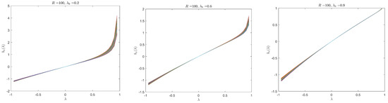
Figure 1. $b_n\left(\lambda \right)$ under variance structure V1 and parameter configuration P1, $R=100$.

One may wonder about the performance of the proposed II estimator under homoscedasticity, relative to the QML estimator of Lee (2004) and the best GMM estimator of Lee (2007).9 Table 5 and Table 6 report the Monte Carlo results under parameter configurations P1 and P2, but now the error term is simulated as a standard normal random variable. The exogenous variables were simulated the same as before. From Table 5 and Table 6, one observes that the II estimator is slightly better than the best GMM estimator of Lee (2007), usually delivering smaller finite-sample bias and lower RMSE. Both methods have good finite-sample size performance in terms of the $5\%$ t test. The finite-sample performance of the QML, on the other hand, is quite different from what the asymptotic theory predicts. Its bias is more severe than the other two and it also gives higher RMSE. Moreover, its size performance is very poor.

Table 5. Estimation of SAR under homoscedasticity with parameter configuration P1.

			QML				GMM				II
R	${\mathit{\theta }}_0$		Bias	RMSE	$\mathit{P}(5\%)$		Bias	RMSE	$\mathit{P}(5\%)$		Bias	RMSE	$\mathit{P}(5\%)$
100	0.2		0.014	0.043	19.0%		−0.007	0.040	7.5%		−0.003	0.037	5.6%
	0.8		−0.032	0.146	18.5%		0.025	0.144	6.7%		0.013	0.138	6.3%
	0.2		−0.002	0.029	15.9%		−0.002	0.029	6.1%		−0.002	0.029	6.1%
	1.5		−0.001	0.026	17.7%		−0.002	0.026	6.1%		−0.001	0.026	5.9%
	0.6		0.026	0.032	34.1%		−0.004	0.020	5.4%		−0.002	0.019	5.2%
	0.8		−0.137	0.188	26.5%		0.022	0.137	5.4%		0.010	0.131	4.7%
	0.2		−0.001	0.029	17.3%		−0.001	0.029	5.1%		0.000	0.029	5.1%
	1.5		−0.005	0.026	15.3%		0.000	0.026	4.5%		0.001	0.026	4.4%
	0.9		0.011	0.011	51.3%		−0.001	0.005	5.2%		0.000	0.005	4.1%
	0.8		−0.213	0.248	39.9%		0.022	0.140	5.5%		0.009	0.134	5.0%
	0.2		−0.002	0.028	14.5%		−0.001	0.028	4.3%		−0.001	0.028	3.9%
	1.5		−0.011	0.029	19.8%		0.001	0.027	5.1%		0.001	0.027	4.7%
200	0.2		0.017	0.032	23.0%		−0.003	0.026	5.6%		−0.001	0.025	4.3%
	0.8		−0.044	0.103	18.6%		0.009	0.094	5.0%		0.003	0.090	3.6%
	0.2		−0.001	0.020	15.7%		−0.001	0.020	4.1%		−0.001	0.020	4.2%
	1.5		0.001	0.017	14.1%		0.001	0.017	4.6%		0.001	0.017	4.9%
	0.6		0.028	0.030	62.1%		−0.002	0.014	5.3%		−0.001	0.013	4.2%
	0.8		−0.145	0.172	47.1%		0.009	0.096	4.8%		0.003	0.093	3.8%
	0.2		0.000	0.021	18.4%		0.000	0.021	4.5%		0.000	0.021	4.5%
	1.5		−0.005	0.019	18.1%		0.000	0.018	5.3%		0.001	0.018	4.8%
	0.9		0.011	0.011	85.1%		0.000	0.004	6.3%		0.000	0.003	4.1%
	0.8		−0.220	0.237	68.7%		0.009	0.097	5.9%		0.004	0.093	5.0%
	0.2		−0.002	0.021	17.7%		0.000	0.021	4.5%		0.000	0.021	4.4%
	1.5		−0.014	0.023	25.0%		−0.002	0.019	4.6%		−0.001	0.019	4.5%

The weight matrix is a social interaction matrix ${\mathit{W}}_n={\mathit{I}}_R\otimes [({\mathbf{1}}_{m_j}{\mathbf{1}}_{m_j}^{\prime }-{\mathit{I}}_{m_j})/(m_j-1)]$, $m_j\sim \mathrm{IID}\mathrm{U}(3,20)$, $j=1,\cdots ,R$. Reported for each estimator are the bias, RMSE, and the empirical size of the t test for each parameter equal to its true value at $5\%$ from 1000 simulations. The exogenous regressors are ${(1,x_{i1},x_{i2})}^{\prime }$, $x_{i1}\sim \mathrm{IID}\mathrm{N}(3,1)$, $x_{i2}\sim \mathrm{IID}\mathrm{U}(-1,2)$, and $x_{i1}$ is independent of $x_{i2}$. The group size $m_j$ follows $\mathrm{IID}\mathrm{U}(3,20)$. The error terms follow a standard normal distribution.

Table 6. Estimation of SAR under homoscedasticity with parameter configuration P2.

			QML				GMM				II
R	${\mathit{\theta }}_0$		Bias	RMSE	$\mathit{P}(5\%)$		Bias	RMSE	$\mathit{P}(5\%)$		Bias	RMSE	$\mathit{P}(5\%)$
100	0.2		0.041	0.078	13.3%		−0.007	0.056	5.7%		−0.004	0.055	5.6%
	0.2		−0.037	0.121	14.7%		0.017	0.112	5.3%		0.011	0.109	5.1%
	0.2		−0.002	0.029	16.2%		−0.004	0.029	5.9%		−0.002	0.029	6.0%
	0.1		0.000	0.026	18.0%		−0.001	0.026	6.6%		0.000	0.026	6.4%
	0.6		0.072	0.076	29.7%		−0.004	0.029	4.6%		−0.002	0.028	4.3%
	0.2		−0.149	0.181	25.9%		0.007	0.108	5.3%		0.001	0.107	5.6%
	0.2		−0.001	0.029	16.4%		−0.001	0.029	5.2%		0.001	0.029	5.2%
	0.1		0.000	0.026	18.2%		0.000	0.027	6.6%		0.001	0.027	6.2%
	0.9		0.026	0.027	48.5%		−0.001	0.008	5.3%		−0.001	0.008	5.3%
	0.2		−0.214	0.235	38.4%		0.010	0.110	5.3%		0.004	0.109	4.9%
	0.2		−0.003	0.028	15.8%		0.000	0.028	4.0%		0.001	0.028	4.2%
	0.1		−0.002	0.025	15.2%		0.000	0.026	5.1%		0.001	0.026	4.9%
200	0.2		0.046	0.064	23.3%		−0.004	0.038	4.6%		−0.003	0.038	4.5%
	0.2		−0.046	0.093	18.7%		0.009	0.079	5.3%		0.005	0.078	4.7%
	0.2		−0.001	0.021	17.5%		−0.002	0.021	6.0%		−0.001	0.021	5.6%
	0.1		0.000	0.018	15.8%		0.000	0.018	4.3%		0.000	0.018	4.0%
	0.6		0.074	0.076	70.7%		−0.002	0.020	4.8%		−0.001	0.020	4.6%
	0.2		−0.152	0.170	49.3%		0.004	0.081	6.3%		0.000	0.079	5.9%
	0.2		−0.002	0.021	17.6%		−0.001	0.021	5.0%		0.001	0.021	5.0%
	0.1		0.000	0.019	17.8%		0.000	0.019	6.1%		0.001	0.019	6.4%
	0.9		0.027	0.027	95.2%		−0.001	0.005	4.6%		0.000	0.005	4.1%
	0.2		−0.218	0.229	72.6%		0.005	0.081	6.0%		0.001	0.079	5.2%
	0.2		−0.003	0.020	15.3%		0.000	0.020	4.8%		0.001	0.020	4.8%
	0.1		−0.001	0.018	15.0%		0.000	0.018	4.2%		0.001	0.018	3.9%

The weight matrix is a social interaction matrix ${\mathit{W}}_n={\mathit{I}}_R\otimes [({\mathbf{1}}_{m_j}{\mathbf{1}}_{m_j}^{\prime }-{\mathit{I}}_{m_j})/(m_j-1)]$, $m_j\sim \mathrm{IID}\mathrm{U}(3,20)$, $j=1,\cdots ,R$. Reported for each estimator are the bias, RMSE, and the empirical size of the t test for each parameter equal to its true value at $5\%$ from 1000 simulations. The exogenous regressors are ${(1,x_{i1},x_{i2})}^{\prime }$, $x_{i1}\sim \mathrm{IID}\mathrm{N}(3,1)$, $x_{i2}\sim \mathrm{IID}\mathrm{U}(-1,2)$, and $x_{i1}$ is independent of $x_{i2}$. The group size $m_j$ follows $\mathrm{IID}\mathrm{U}(3,20)$. The error terms follow a standard normal distribution.

The simulation results suggest that the II estimator could be used at least as a complement to other consistent estimators proposed in the literature that are robust to unknown heteroscedasticity. The II method may be favored for the purpose of hypothesis testing, especially for testing the spatial autoregression parameter. It also has very good finite-sample performance under homoscedasticity.

5. Concluding Remarks

Lee (2002) challenged the traditional wisdom that the OLS estimator is biased and inconsistent in spatial autoregressions and showed that it may be consistent under some special circumstances if there are exogenous regressors included. This paper thoroughly examines the asymptotic behavior of the OLS estimator under different specifications of the degree of aggregate influence on each unit from other units and provides a unified asymptotic distribution result of the recentered OLS estimator. Based on this, an indirect inference estimator, which is consistent and asymptotically normal, is introduced. The new estimator is relatively easy to calculate, does not rely on distributional assumptions on the data, and is robust to heteroscedasticity. Monte Carlo experiments in this paper show the good finite-sample performance of the II estimator in comparison with other consistent estimators that are robust to unknown heteroscedasticity.

In this paper, no attempt is made to conduct some comparison of the asymptotic variances of the GMM and II estimators. The II estimator in this paper may be interpreted as an estimator that uses one moment condition, namely, by matching the OLS estimator ${\widehat{\lambda }}_n$ with its approximate analytical expectation. In contrast, the GMM estimator in Lin and Lee (2010) is based on a set of exact expectations of bilinear and quadratic forms in ${\mathit{u}}_n$. The OLS estimator itself is based on an incorrect moment condition, namely, exogeneity of ${\mathit{W}}_n{\mathit{y}}_n$. It is not clear whether correcting an incorrect moment condition is as efficient as using a set of correct moment conditions. A fruitful strategy is perhaps to design a combined estimator.10 Another possible extension is to consider the more general higher-order SARAR (spatial autoregressive model with spatial autoregressive disturbances) with heteroscedastic innovations as in Badinger and Egger (2011) and Jin and Lee (2019). In this more general setup, the II procedure may be implemented as follows. One can first derive the approximate analytical expectation of the OLS estimator of the parameters in the SAR part, taken the parameters in the disturbance part as given, and thus design a “corrected” SAR estimator. Then based on the residuals that arise from the “corrected” SAR estimator, one can derive approximate analytical expectation of the OLS estimator of the parameters in the disturbance part. In the end, one can jointly estimate all the parameters in the SAR and disturbance parts by using the two sets of approximate analytical expectations. Some preliminary simulations show very promising results from this approach. Rigorous treatments of these extensions are left for future studies.

Appendix B.1. Proof of Theorem 1

Proof. 

By a Nagar-type (Nagar (1959)) expansion,

$$\begin{array}{cc}\hfill \sqrt{n}\left({\widehat{\lambda }}_n-{\lambda }_0-\frac{\mathrm{tr}\left({\mathsf{\Sigma }}_n{\mathit{M}}_n{\mathit{G}}_n\right)}{{\mathit{y}}_n^{\prime }{\mathit{W}}_n^{\prime }{\mathit{M}}_n{\mathit{W}}_n{\mathit{y}}_n}\right)& =\sqrt{n}\left(\frac{r_{1n}-\mathrm{E}\left(r_{1n}\right)+r_{2n}}{d_n}\right)\hfill \\ \hfill & =\sqrt{n}\left(\frac{r_{1n}-\mathrm{E}\left(r_{1n}\right)+r_{2n}}{\mathrm{E}\left(d_n\right)+d_n-\mathrm{E}\left(d_n\right)}\right)\hfill \\ \hfill & =\sqrt{n}\left(\frac{r_{1n}-\mathrm{E}\left(r_{1n}\right)+r_{2n}}{\mathrm{E}\left(d_n\right)}\right){\left(1+\frac{d_n-\mathrm{E}\left(d_n\right)}{\mathrm{E}\left(d_n\right)}\right)}^{-1}\hfill \\ \hfill & =\sqrt{n}\left(\frac{r_{1n}-\mathrm{E}\left(r_{1n}\right)+r_{2n}}{\mathrm{E}\left(d_n\right)}\right)+o_P\left(1\right)\hfill \end{array}$$

where, in light of the proof of Lemma A6, $r_{1n}-\mathrm{E}\left(r_{1n}\right)=O_P\left(\sqrt{n/h_n}\right)$, $r_{2n}=O\left(\sqrt{n}\right)$, and $\mathrm{E}\left(d_n\right)=O\left(n\right)$. So when $h_n$ diverges,

$$\sqrt{n}\left({\widehat{\lambda }}_n-{\lambda }_0-\frac{\mathrm{tr}\left({\mathsf{\Sigma }}_n{\mathit{M}}_n{\mathit{G}}_n\right)}{{\mathit{y}}_n^{\prime }{\mathit{W}}_n^{\prime }{\mathit{M}}_n{\mathit{W}}_n{\mathit{y}}_n}\right)=\frac{\sqrt{n}{r}_{2n}}{\mathrm{E}\left(d_n\right)}+o_P\left(1\right),$$

and one can apply Lemma A7 to $r_{2n}={\mathit{\beta }}_0^{\prime }{\mathit{X}}_n^{\prime }{\mathit{G}}_n^{\prime }{\mathit{M}}_n{\mathit{u}}_n$; when $h_n$ is bounded, one can apply Lemma A7 to $r_n=r_{1n}+r_{2n}={\mathit{u}}_n^{\prime }{\mathit{M}}_n{\mathit{G}}_n{\mathit{u}}_n+{\mathit{\beta }}_0^{\prime }{\mathit{X}}_n^{\prime }{\mathit{G}}_n^{\prime }{\mathit{M}}_n{\mathit{u}}_n$. From Lemma A6, one sees that $\mathrm{Var}\left(r_{2n}\right)=\mathrm{Var}\left(r_n\right)+o\left(n\right)$ when $h_n$ diverges. Therefore, regardless of $h_n$,

$$\sqrt{n}\left({\widehat{\lambda }}_n-{\lambda }_0-\frac{\mathrm{tr}\left({\mathsf{\Sigma }}_n{\mathit{M}}_n{\mathit{G}}_n\right)}{{\mathit{y}}_n^{\prime }{\mathit{W}}_n^{\prime }{\mathit{M}}_n{\mathit{W}}_n{\mathit{y}}_n}\right)\stackrel{d}{\to }\mathrm{N}\left(0,\underset{n\to \infty }{lim}\frac{n\mathrm{Var}\left(r_n\right)}{{\left[\mathrm{E}\left(d_n\right)\right]}^2}\right).$$

 □

Appendix B.2. Proof of Theorem 2

Proof. 

Note that

$$\begin{array}{cc}\hfill {\tilde{\mathit{u}}}_n^{\prime }{\mathit{D}}_n{\tilde{\mathit{u}}}_n& ={\mathit{u}}_n^{\prime }{\mathit{D}}_n{\mathit{u}}_n+{({\tilde{\mathit{\beta }}}_n-{\mathit{\beta }}_0)}^{\prime }{\mathit{X}}_n^{\prime }{\mathit{X}}_n({\tilde{\mathit{\beta }}}_n-{\mathit{\beta }}_0)-2{({\tilde{\mathit{\beta }}}_n-{\mathit{\beta }}_0)}^{\prime }{\mathit{X}}_n^{\prime }{\mathit{D}}_n{\mathit{u}}_n\hfill \\ \hfill & ={\mathit{u}}_n^{\prime }{\mathit{D}}_n{\mathit{u}}_n+O_P\left(1\right)+O_P\left(n^{-1/2}\right)O_P\left(\sqrt{n/h_n^2}\right),\hfill \end{array}$$

in view of ${\mathit{X}}_n^{\prime }{\mathit{X}}_n=O\left(n\right)$, ${\tilde{\mathit{\beta }}}_n-{\mathit{\beta }}_0=O_P\left(n^{-1/2}\right)$ and $\mathrm{Var}\left({\mathit{X}}_n^{\prime }{\mathit{D}}_n{\mathit{u}}_n\right)={\mathit{X}}_n^{\prime }{\mathit{D}}_n{\mathsf{\Sigma }}_n{\mathit{D}}_n{\mathit{X}}_n=O(n/h_n^2)$. Then

$$\begin{array}{cc}\hfill & \sqrt{n}\left({\widehat{\lambda }}_n-{\lambda }_0-\frac{{\mathit{y}}_n^{\prime }{\mathit{S}}_n^{\prime }{\mathit{M}}_n{\mathit{D}}_n{\mathit{M}}_n{\mathit{S}}_n{\mathit{y}}_n}{{\mathit{y}}_n^{\prime }{\mathit{W}}_n^{\prime }{\mathit{M}}_n{\mathit{W}}_n{\mathit{y}}_n}\right)\hfill \\ \hfill & =\sqrt{n}\left({\widehat{\lambda }}_n-{\lambda }_0-\frac{{\mathit{u}}_n^{\prime }{\mathit{D}}_n{\mathit{u}}_n}{d_n}+\frac{{\mathit{u}}_n^{\prime }{\mathit{D}}_n{\mathit{u}}_n-{\tilde{\mathit{u}}}_n^{\prime }{\mathit{D}}_n{\tilde{\mathit{u}}}_n}{d_n}\right)\hfill \\ \hfill & =\sqrt{n}\left(\frac{r_n-{\mathit{u}}_n^{\prime }{\mathit{D}}_n{\mathit{u}}_n}{d_n}\right)+o_P\left(1\right)\hfill \\ \hfill & =\sqrt{n}\left(\frac{r_n-{\mathit{u}}_n^{\prime }{\mathit{D}}_n{\mathit{u}}_n}{\mathrm{E}\left(d_n\right)}\right)+o_P\left(1\right).\hfill \end{array}$$

It follows from Lemma A7 that

$$\sqrt{n}\left({\widehat{\lambda }}_n-{\lambda }_0-\frac{{\mathit{y}}_n^{\prime }{\mathit{S}}_n^{\prime }{\mathit{M}}_n{\mathit{D}}_n{\mathit{M}}_n{\mathit{S}}_n{\mathit{y}}_n}{{\mathit{y}}_n^{\prime }{\mathit{W}}_n^{\prime }{\mathit{M}}_n{\mathit{W}}_n{\mathit{y}}_n}\right)\stackrel{d}{\to }\mathrm{N}(0,\eta ),$$

where

$$\begin{array}{cc}\hfill \eta & =\underset{n\to \infty }{lim}n\frac{\mathrm{Var}(r_n-{\mathit{u}}_n^{\prime }{\mathit{D}}_n{\mathit{u}}_n)}{{\left[\mathrm{E}\left(d_n\right)\right]}^2}\hfill \\ \hfill & =\underset{n\to \infty }{lim}n\frac{\mathrm{Var}({\mathit{u}}_n^{\prime }{\mathit{E}}_n{\mathit{u}}_n+{\mathit{\beta }}_0^{\prime }{\mathit{X}}_n^{\prime }{\mathit{G}}_n^{\prime }{\mathit{M}}_n{\mathit{u}}_n)}{{\left[\mathrm{E}\left(d_n\right)\right]}^2}\hfill \\ \hfill & =\underset{n\to \infty }{lim}\frac{n\left\{\mathrm{tr}\left[{\mathsf{\Sigma }}_n{\mathit{E}}_n{\mathsf{\Sigma }}_n({\mathit{E}}_n+{\mathit{E}}_n^{\prime })\right]+{\mathit{\beta }}_0^{\prime }{\mathit{X}}_n^{\prime }{\mathit{G}}_n^{\prime }{\mathit{M}}_n{\mathsf{\Sigma }}_n{\mathit{M}}_n{\mathit{G}}_n{\mathit{X}}_n{\mathit{\beta }}_0\right\}}{[\mathrm{E}{\left(d_n\right]}^2}\hfill \end{array}$$

(A.9)

by using Lemma A4 and the fact that $\mathrm{dg}\left({\mathit{E}}_n\right)=\mathbf{0}$. □

Appendix B.3. Proof of Theorem 3

Proof. 

One can apply the extended delta method as in Phillips (2012) to derive the asymptotic distribution of $\sqrt{n}({\widehat{\lambda }}_n^{II}-{\lambda }_0)$. For this purpose, one needs to check a technical condition, namely, the $\partial b_n^{-1}\left(\lambda \right)/\partial \lambda$ should be asymptotically locally equicontinuous at ${\lambda }_0$: for given $\zeta >0$, if $s_n\to \infty$ and $s_n/\sqrt{n}\to 0$,

$$\underset{s_n\left|\lambda -{\lambda }_0\right|<\zeta }{sup}\left|\frac{b_n^{-1\prime }\left(\lambda \right)-b_n^{-1\prime }\left({\lambda }_0\right)}{b_n^{-1\prime }\left({\lambda }_0\right)}\right|=\underset{s_n\left|\lambda -{\lambda }_0\right|<\zeta }{sup}\left|\frac{b_n^{\prime }\left({\lambda }_0\right)-b_n^{\prime }\left(\lambda \right)}{b_n^{\prime }\left(\lambda \right)}\right|\stackrel{a.s.}{\to }0.$$

The first derivative of the binding function is

$$\begin{array}{cc}\hfill & b_n^{\prime }\left(\lambda \right)\hfill \\ \hfill & =1+\frac{{\mathit{y}}_n^{\prime }{\mathit{S}}_n^{\prime }\left(\lambda \right){\mathit{M}}_n\mathrm{Dg}\left({\mathit{M}}_n{\mathit{G}}_n^2\left(\lambda \right)\right){\mathit{M}}_n{\mathit{S}}_n\left(\lambda \right){\mathit{y}}_n-2{\mathit{y}}_n^{\prime }{\mathit{W}}_n^{\prime }{\mathit{M}}_n\mathrm{Dg}\left({\mathit{M}}_n{\mathit{G}}_n\left(\lambda \right)\right){\mathit{M}}_n{\mathit{S}}_n\left(\lambda \right){\mathit{y}}_n}{{\mathit{y}}_n^{\prime }{\mathit{W}}_n^{\prime }{\mathit{M}}_n{\mathit{W}}_n{\mathit{y}}_n}.\hfill \end{array}$$

(A.10)

By substituting ${\mathit{y}}_n={\mathit{S}}_n^{-1}{\mathit{X}}_n{\mathit{\beta }}_0+{\mathit{S}}_n^{-1}{\mathit{u}}_n$ and using Lemmas A2–A4, one can see that the second term in (A.10) converges almost surely to a bounded constant for all $\lambda \in \mathsf{\Lambda }$. In a similar way, one can show

$$\begin{array}{cc}\hfill & b_n^{″}\left(\lambda \right)\hfill \\ \hfill & =\frac{2{\mathit{y}}_n^{\prime }{\mathit{S}}_n^{\prime }\left(\lambda \right){\mathit{M}}_n\mathrm{Dg}\left({\mathit{M}}_n{\mathit{G}}_n^3\left(\lambda \right)\right){\mathit{M}}_n{\mathit{S}}_n\left(\lambda \right){\mathit{y}}_n+2{\mathit{y}}_n^{\prime }{\mathit{W}}_n^{\prime }{\mathit{M}}_n\mathrm{Dg}\left({\mathit{M}}_n{\mathit{G}}_n\left(\lambda \right)\right){\mathit{M}}_n{\mathit{W}}_n{\mathit{y}}_n}{{\mathit{y}}_n^{\prime }{\mathit{W}}_n^{\prime }{\mathit{M}}_n{\mathit{W}}_n{\mathit{y}}_n}\hfill \end{array}$$

also converges almost surely to a bounded constant. Thus, for some ${\lambda }^{*}$ that lies between ${\lambda }_0$ and $\lambda$,

$$\left|\frac{b_n^{\prime }\left({\lambda }_0\right)-b_n^{\prime }\left(\lambda \right)}{b_n^{\prime }\left(\lambda \right)}\right|=\left|\lambda -{\lambda }_0\right|\left|\frac{b_n^{″}\left({\lambda }^{*}\right)}{b_n^{\prime }\left(\lambda \right)}\right|<\frac{\zeta }{s_n}\left|\frac{b_n^{″}\left({\lambda }^{*}\right)}{b_n^{\prime }\left(\lambda \right)}\right|\stackrel{a.s.}{\to }0.$$

With all these results, (12) follows immediately from Theorem 1 of Phillips (2012) and Theorem 2 in this paper. □

Appendix B.4. Proof of Theorem 4

Proof. 

Upon substitution,

$$\begin{array}{cc}\hfill {\widehat{\mathit{\beta }}}_n^{II}& ={\left({\mathit{X}}_n^{\prime }{\mathit{X}}_n\right)}^{-1}{\mathit{X}}_n^{\prime }{\widehat{\mathit{S}}}_n{\mathit{S}}_n^{-1}{\mathit{X}}_n{\mathit{\beta }}_0+{\left({\mathit{X}}_n^{\prime }{\mathit{X}}_n\right)}^{-1}{\mathit{X}}_n^{\prime }{\widehat{\mathit{S}}}_n{\mathit{S}}_n^{-1}{\mathit{u}}_n\hfill \\ \hfill & ={\left({\mathit{X}}_n^{\prime }{\mathit{X}}_n\right)}^{-1}{\mathit{X}}_n^{\prime }\left[{\mathit{S}}_n-({\widehat{\lambda }}_n^{II}-{\lambda }_0){\mathit{W}}_n\right]{\mathit{S}}_n^{-1}{\mathit{X}}_n{\mathit{\beta }}_0\hfill \\ \hfill & +{\left({\mathit{X}}_n^{\prime }{\mathit{X}}_n\right)}^{-1}{\mathit{X}}_n^{\prime }\left[{\mathit{S}}_n-({\widehat{\lambda }}_n^{II}-{\lambda }_0){\mathit{W}}_n\right]{\mathit{S}}_n^{-1}{\mathit{u}}_n\hfill \\ \hfill & ={\mathit{\beta }}_0+{\left({\mathit{X}}_n^{\prime }{\mathit{X}}_n\right)}^{-1}{\mathit{X}}_n^{\prime }{\mathit{u}}_n-({\widehat{\lambda }}_n^{II}-{\lambda }_0)\left[{\left({\mathit{X}}_n^{\prime }{\mathit{X}}_n\right)}^{-1}{\mathit{X}}_n^{\prime }{\mathit{G}}_n{\mathit{X}}_n{\mathit{\beta }}_0+{\left({\mathit{X}}_n^{\prime }{\mathit{X}}_n\right)}^{-1}{\mathit{X}}_n^{\prime }{\mathit{G}}_n{\mathit{u}}_n\right],\hfill \end{array}$$

where ${\widehat{\lambda }}_n^{II}-{\lambda }_0=O_p\left(n^{-1/2}\right)$ (from Theorem 3). Further, ${\left({\mathit{X}}_n^{\prime }{\mathit{X}}_n\right)}^{-1}{\mathit{X}}_n^{\prime }{\mathit{u}}_n=O_p\left(n^{-1/2}\right)$, ${\left({\mathit{X}}_n^{\prime }{\mathit{X}}_n\right)}^{-1}{\mathit{X}}_n^{\prime }{\mathit{G}}_n{\mathit{X}}_n{\mathit{\beta }}_0=O\left(1\right)$, and ${\left({\mathit{X}}_n^{\prime }{\mathit{X}}_n\right)}^{-1}{\mathit{X}}_n^{\prime }{\mathit{G}}_n{\mathit{u}}_n=O_p\left(n^{-1/2}\right)$ (from Lemma A5). Note that if one expands ${\widehat{\lambda }}_n^{II}-{\lambda }_0=b_n^{-1}\left({\widehat{\lambda }}_n\right)-b_n^{-1}\left(b_n\left({\lambda }_0\right)\right)$,

$$\sqrt{n}({\widehat{\lambda }}_n^{II}-{\lambda }_0)=\frac{\sqrt{n}\left({\widehat{\lambda }}_n-b_n\left({\lambda }_0\right)\right)}{b_n^{\prime }\left({\lambda }_0\right)}+O_P\left(n^{-1/2}\right).$$

(A.11)

From the proof of Theorem 2,

$${\widehat{\lambda }}_n-b_n\left({\lambda }_0\right)=\frac{r_n-{\mathit{u}}_n^{\prime }{\mathit{D}}_n{\mathit{u}}_n}{\mathrm{E}\left(d_n\right)}+o_P\left(n^{-1/2}\right)=\frac{{\mathit{u}}_n^{\prime }{\mathit{E}}_n{\mathit{u}}_n+{\mathit{\beta }}_0^{\prime }{\mathit{X}}_n^{\prime }{\mathit{G}}_n^{\prime }{\mathit{M}}_n{\mathit{u}}_n}{\mathrm{E}\left(d_n\right)}+o_P\left(n^{-1/2}\right).$$

(A.12)

Given the above results, one has

$$\begin{array}{cc}\hfill & \sqrt{n}({\widehat{\mathit{\beta }}}_n^{II}-{\mathit{\beta }}_0)\hfill \\ \hfill & =\sqrt{n}{\left({\mathit{X}}_n^{\prime }{\mathit{X}}_n\right)}^{-1}{\mathit{X}}_n^{\prime }{\mathit{u}}_n-\sqrt{n}({\widehat{\lambda }}_n^{II}-{\lambda }_0){\left({\mathit{X}}_n^{\prime }{\mathit{X}}_n\right)}^{-1}{\mathit{X}}_n^{\prime }{\mathit{G}}_n{\mathit{X}}_n{\mathit{\beta }}_0+o_P\left(1\right)\hfill \\ \hfill & =\sqrt{n}{\left({\mathit{X}}_n^{\prime }{\mathit{X}}_n\right)}^{-1}{\mathit{X}}_n^{\prime }{\mathit{u}}_n-\left[\frac{\sqrt{n}\left({\widehat{\lambda }}_n-b_n\left({\lambda }_0\right)\right)}{b_n^{\prime }\left({\lambda }_0\right)}\right]{\left({\mathit{X}}_n^{\prime }{\mathit{X}}_n\right)}^{-1}{\mathit{X}}_n^{\prime }{\mathit{G}}_n{\mathit{X}}_n{\mathit{\beta }}_0+o_P\left(1\right)\hfill \\ \hfill & =\sqrt{n}{\left({\mathit{X}}_n^{\prime }{\mathit{X}}_n\right)}^{-1}{\mathit{X}}_n^{\prime }{\mathit{u}}_n-\frac{\sqrt{n}{\left({\mathit{X}}_n^{\prime }{\mathit{X}}_n\right)}^{-1}{\mathit{X}}_n^{\prime }{\mathit{G}}_n{\mathit{X}}_n{\mathit{\beta }}_0}{b_n^{\prime }\left({\lambda }_0\right)}\frac{{\mathit{u}}_n^{\prime }{\mathit{E}}_n{\mathit{u}}_n+{\mathit{\beta }}_0^{\prime }{\mathit{X}}_n^{\prime }{\mathit{G}}_n^{\prime }{\mathit{M}}_n{\mathit{u}}_n}{\mathrm{E}\left(d_n\right)}+o_P\left(1\right).\hfill \end{array}$$

(A.13)

One can check that Lemma A7 can be applied to each element or any nonstochastic linear combination of elements of $\sqrt{n}({\widehat{\mathit{\beta }}}_n^{II}-{\mathit{\beta }}_0)$ under such a representation. So $\sqrt{n}({\widehat{\mathit{\beta }}}_n^{II}-{\mathit{\beta }}_0)$ converges to a normal distribution, with the asymptotic covariance matrix,

$$\begin{array}{cc}\hfill \mathit{V}=& \underset{n\to \infty }{lim}\{n{\left({\mathit{X}}_n^{\prime }{\mathit{X}}_n\right)}^{-1}{\mathit{X}}_n^{\prime }{\mathsf{\Sigma }}_n{\mathit{X}}_n{\left({\mathit{X}}_n^{\prime }{\mathit{X}}_n\right)}^{-1}\hfill \\ \hfill & +\frac{\eta }{b_0^2}{\left({\mathit{X}}_n^{\prime }{\mathit{X}}_n\right)}^{-1}{\mathit{X}}_n^{\prime }{\mathit{G}}_n{\mathit{X}}_n{\mathit{\beta }}_0{\mathit{\beta }}_0^{\prime }{\mathit{X}}_n^{\prime }{\mathit{G}}_n^{\prime }{\mathit{X}}_n{\left({\mathit{X}}_n^{\prime }{\mathit{X}}_n\right)}^{-1}\hfill \\ \hfill & -\frac{n{\left({\mathit{X}}_n^{\prime }{\mathit{X}}_n\right)}^{-1}{\mathit{X}}_n^{\prime }{\mathit{G}}_n{\mathit{X}}_n{\mathit{\beta }}_0{\mathit{\beta }}_0^{\prime }{\mathit{X}}_n^{\prime }{\mathit{G}}_n^{\prime }{\mathit{M}}_n{\mathsf{\Sigma }}_n{\mathit{X}}_n{\left({\mathit{X}}_n^{\prime }{\mathit{X}}_n\right)}^{-1}}{b_0[\mathrm{tr}\left({\mathsf{\Sigma }}_n{\mathit{G}}_n^{\prime }{\mathit{M}}_n{\mathit{G}}_n\right)+{\mathit{\beta }}_0^{\prime }{\mathit{X}}_n^{\prime }{\mathit{G}}_n^{\prime }{\mathit{M}}_n{\mathit{G}}_n{\mathit{X}}_n{\mathit{\beta }}_0]}\hfill \\ \hfill & -\left.\frac{n{\left({\mathit{X}}_n^{\prime }{\mathit{X}}_n\right)}^{-1}{\mathit{X}}_n^{\prime }{\mathsf{\Sigma }}_n{\mathit{M}}_n{\mathit{G}}_n{\mathit{X}}_n{\mathit{\beta }}_0{\mathit{\beta }}_0^{\prime }{\mathit{X}}_n^{\prime }{\mathit{G}}_n^{\prime }{\mathit{X}}_n{\left({\mathit{X}}_n^{\prime }{\mathit{X}}_n\right)}^{-1}}{b_0[\mathrm{tr}\left({\mathsf{\Sigma }}_n{\mathit{G}}_n^{\prime }{\mathit{M}}_n{\mathit{G}}_n\right)+{\mathit{\beta }}_0^{\prime }{\mathit{X}}_n^{\prime }{\mathit{G}}_n^{\prime }{\mathit{M}}_n{\mathit{G}}_n{\mathit{X}}_n{\mathit{\beta }}_0]}\right\}.\hfill \end{array}$$

(A.14)

The asymptotic covariance between ${\widehat{\mathit{\beta }}}_n^{II}$ and ${\widehat{\lambda }}_n^{II}$ follows from the expansion of $\sqrt{n}({\widehat{\lambda }}_n^{II}-{\lambda }_0)$ (see (A.11) and (A.12)) and that of $\sqrt{n}({\widehat{\mathit{\beta }}}_n^{II}-{\mathit{\beta }}_0)$ (see (A.13)), given by

$$\begin{array}{cc}\hfill \mathit{\gamma }& =\underset{n\to \infty }{lim}\left[\frac{n}{b_0\mathrm{E}\left(d_n\right)}{\left({\mathit{X}}_n^{\prime }{\mathit{X}}_n\right)}^{-1}{\mathit{X}}_n^{\prime }{\mathsf{\Sigma }}_n{\mathit{M}}_n{\mathit{G}}_n{\mathit{X}}_n{\mathit{\beta }}_0-\frac{\eta }{b_0^2}{\left({\mathit{X}}_n^{\prime }{\mathit{X}}_n\right)}^{-1}{\mathit{X}}_n^{\prime }{\mathit{G}}_n{\mathit{X}}_n{\mathit{\beta }}_0\right].\hfill \end{array}$$

(A.15)

 □

Appendix B.5. Proof of Corollary 2

Proof. 

By substitution and using the Nagar (1959) expansion,

$$\begin{array}{cc}\hfill \sqrt{\frac{n}{h_n}}\left({\widehat{\lambda }}_n-{\lambda }_0-\frac{{\mathit{y}}_n^{\prime }{\mathit{S}}_n^{\prime }{\mathit{D}}_n{\mathit{S}}_n{\mathit{y}}_n}{{\mathit{y}}_n^{\prime }{\mathit{W}}_n^{\prime }{\mathit{W}}_n{\mathit{y}}_n}\right)& =\sqrt{\frac{n}{h_n}}\left(\frac{r_{1n}}{d_{1n}}-\frac{{\mathit{u}}_n^{\prime }{\mathit{D}}_n{\mathit{u}}_n}{d_{1n}}\right)\hfill \\ \hfill & =\sqrt{\frac{n}{h_n}}\left(\frac{{\mathit{u}}_n^{\prime }{\mathit{E}}_n{\mathit{u}}_n}{d_{1n}}\right)\hfill \\ \hfill & =\sqrt{\frac{n}{h_n}}\frac{{\mathit{u}}_n^{\prime }{\mathit{E}}_n{\mathit{u}}_n}{\mathrm{E}\left(d_{1n}\right)}+o_P\left(1\right),\hfill \end{array}$$

where $\mathrm{E}\left({\mathit{u}}_n^{\prime }{\mathit{E}}_n{\mathit{u}}_n\right)=0$, $\mathrm{Var}\left({\mathit{u}}_n^{\prime }{\mathit{E}}_n{\mathit{u}}_n\right)=\mathrm{tr}\left[{\mathsf{\Sigma }}_n{\mathit{E}}_n{\mathsf{\Sigma }}_n({\mathit{E}}_n+{\mathit{E}}_n^{\prime })\right]=O(n/h_n)$, and and the asymptotic distribution follows when one applies Lemma A7 to the quadratic form ${\mathit{u}}_n^{\prime }{\mathit{E}}_n{\mathit{u}}_n.$ □

Appendix B.6. The Case of Homoscedastic Error Term

If ${\mathsf{\Sigma }}_n={\sigma }_0^2{\mathit{I}}_n$ (and further ${\mathsf{\Sigma }}_n^{\left(j\right)}={\mu }_j{\mathit{I}}_n$, ${\mu }_j=\mathrm{E}\left(u_{i,n}^j\right)$, $j=3,4$), then the recentering term in (7) becomes ${\sigma }_0^2\mathrm{tr}\left({\mathit{M}}_n{\mathit{G}}_n\right)/{\mathit{y}}_n^{\prime }{\mathit{W}}_n^{\prime }{\mathit{M}}_n{\mathit{W}}_n{\mathit{y}}_n$. To make the II procedure feasible, one may replace ${\sigma }_0^2\mathrm{tr}\left({\mathit{M}}_n{\mathit{G}}_n\right)/{\mathit{y}}_n^{\prime }{\mathit{W}}_n^{\prime }{\mathit{M}}_n{\mathit{W}}_n{\mathit{y}}_n$ by $n^{-1}{\mathit{y}}_n^{\prime }{\mathit{S}}_n^{\prime }{\mathit{M}}_n{\mathit{S}}_n{\mathit{y}}_n\mathrm{tr}\left({\mathit{M}}_n{\mathit{G}}_n\right)/{\mathit{y}}_n^{\prime }{\mathit{W}}_n^{\prime }{\mathit{M}}_n{\mathit{W}}_n{\mathit{y}}_n$. Similar to the proof of Theorem 2, one can put

$$\sqrt{n}\left({\widehat{\lambda }}_n-{\lambda }_0-\frac{n^{-1}{\mathit{y}}_n^{\prime }{\mathit{S}}_n^{\prime }{\mathit{M}}_n{\mathit{S}}_n{\mathit{y}}_n\mathrm{tr}\left({\mathit{M}}_n{\mathit{G}}_n\right)}{{\mathit{y}}_n^{\prime }{\mathit{W}}_n^{\prime }{\mathit{M}}_n{\mathit{W}}_n{\mathit{y}}_n}\right)=\sqrt{n}\left(\frac{r_n^{*}-\mathrm{E}\left(r_n^{*}\right)}{\mathrm{E}\left(d_n\right)}\right)+o_P\left(1\right)\stackrel{d}{\to }\mathrm{N}(0,\omega ),$$

where $\omega ={lim}_{n\to \infty }n\mathrm{Var}\left(r_n^{*}\right)/\left\{{\left[\mathrm{E}\left(d_n\right)\right]}^2\right\}$, $r_n^{*}={\mathit{u}}_n^{\prime }{\mathit{M}}_n{\mathit{G}}_n^{*}{\mathit{u}}_n+{\mathit{\beta }}_0^{\prime }{\mathit{X}}_n^{\prime }{\mathit{G}}_n^{\prime }{\mathit{M}}_n{\mathit{u}}_n$, ${\mathit{G}}_n^{*}={\mathit{G}}_n-n^{-1}\mathrm{tr}\left({\mathit{M}}_n{\mathit{G}}_n\right)$. In particular,

$$\begin{array}{cc}\hfill \mathrm{Var}\left(r_n^{*}\right)& ={\mu }_4\mathrm{tr}({\mathit{M}}_n{\mathit{G}}_n^{*}\odot {\mathit{M}}_n{\mathit{G}}_n^{*})+{\sigma }_0^2\mathrm{tr}\left[{\mathit{M}}_n{\mathit{G}}_n^{*}({\mathit{M}}_n{\mathit{G}}_n^{*}+{\mathit{G}}_n^{*\prime }{\mathit{M}}_n)\right]\hfill \\ \hfill & +{\sigma }_0^2{\mathit{\beta }}_0^{\prime }{\mathit{X}}_n^{\prime }{\mathit{G}}_n^{\prime }{\mathit{M}}_n{\mathit{M}}_n{\mathit{G}}_n{\mathit{X}}_n{\mathit{\beta }}_0+2{\mu }_3{\mathit{\beta }}_0^{\prime }{\mathit{X}}_n^{\prime }{\mathit{G}}_n^{\prime }{\mathit{M}}_n\mathrm{dg}\left({\mathit{M}}_n{\mathit{G}}_n^{*}\right).\hfill \end{array}$$

Define the binding function as $b_n\left(\lambda \right)=\lambda +n^{-1}{\mathit{y}}_n^{\prime }{\mathit{S}}_n^{\prime }\left(\lambda \right){\mathit{M}}_n{\mathit{S}}_n\left(\lambda \right){\mathit{y}}_n\mathrm{tr}\left({\mathit{M}}_n{\mathit{G}}_n\left(\lambda \right)\right)/{\mathit{y}}_n^{\prime }{\mathit{W}}_n^{\prime }{\mathit{M}}_n{\mathit{W}}_n{\mathit{y}}_n$ and $b_n^{\prime }\left({\lambda }_0\right)=1+{\left(n{\mathit{y}}_n^{\prime }{\mathit{W}}_n^{\prime }{\mathit{M}}_n{\mathit{W}}_n{\mathit{y}}_n\right)}^{-1}[{\mathit{y}}_n^{\prime }{\mathit{S}}_n^{\prime }{\mathit{M}}_n{\mathit{S}}_n{\mathit{y}}_n\mathrm{tr}\left({\mathit{M}}_n{\mathit{G}}_n^2\right)-2{\mathit{y}}_n^{\prime }{\mathit{W}}_n^{\prime }{\mathit{M}}_n{\mathit{S}}_n{\mathit{y}}_n\mathrm{tr}\left({\mathit{M}}_n{\mathit{G}}_n\right)]$. Assume $b_n^{\prime }\left({\lambda }_0\right)\stackrel{a.s.}{\to }{b}_0\ne 0$. The asymptotic distribution of ${({\widehat{\lambda }}_n^{II},{\widehat{\mathit{\beta }}}_n^{II\prime })}^{\prime }$ resulting from this binding function follows similarly from the proofs of Theorems 3 and 4, given by

$$\sqrt{n}\left(\begin{array}{c}{\widehat{\lambda }}_n^{II}-{\lambda }_0\\ {\widehat{\mathit{\beta }}}_n^{II}-{\mathit{\beta }}_0\end{array}\right)\stackrel{d}{\to }\mathrm{N}\left(\mathbf{0},\left(\begin{array}{cc}\frac{\omega }{b_0^2}& {\mathit{\gamma }}^{\prime }\\ \mathit{\gamma }& \mathit{V}\end{array}\right)\right),$$

where

$$\begin{array}{cc}\hfill \mathit{V}& =\underset{n\to \infty }{lim}\{n{\sigma }_0^2{\left({\mathit{X}}_n^{\prime }{\mathit{X}}_n\right)}^{-1}+\frac{\omega }{b_0^2}{\left({\mathit{X}}_n^{\prime }{\mathit{X}}_n\right)}^{-1}{\mathit{X}}_n^{\prime }{\mathit{G}}_n{\mathit{X}}_n{\mathit{\beta }}_0{\mathit{\beta }}_0^{\prime }{\mathit{X}}_n^{\prime }{\mathit{G}}_n^{\prime }{\mathit{X}}_n{\left({\mathit{X}}_n^{\prime }{\mathit{X}}_n\right)}^{-1}\hfill \\ \hfill & -\frac{n{\left({\mathit{X}}_n^{\prime }{\mathit{X}}_n\right)}^{-1}{\mathit{X}}_n^{\prime }{\mathit{G}}_n{\mathit{X}}_n{\mathit{\beta }}_0[{\sigma }_0^2{\mathit{\beta }}_0^{\prime }{\mathit{X}}_n^{\prime }{\mathit{G}}_n^{\prime }{\mathit{M}}_n+{\mu }_3\mathrm{dg}{\left({\mathit{M}}_n{\mathit{G}}_n^{*}\right)}^{\prime }]{\mathit{X}}_n{\left({\mathit{X}}_n^{\prime }{\mathit{X}}_n\right)}^{-1}}{b_0[{\sigma }_0^2\mathrm{tr}\left({\mathit{G}}_n^{\prime }{\mathit{M}}_n{\mathit{G}}_n\right)+{\mathit{\beta }}_0^{\prime }{\mathit{X}}_n^{\prime }{\mathit{G}}_n^{\prime }{\mathit{M}}_n{\mathit{G}}_n{\mathit{X}}_n{\mathit{\beta }}_0]}\hfill \\ \hfill & -\left.\frac{n{\left({\mathit{X}}_n^{\prime }{\mathit{X}}_n\right)}^{-1}{\mathit{X}}_n^{\prime }[{\sigma }_0^2{\mathit{M}}_n{\mathit{G}}_n{\mathit{X}}_n{\mathit{\beta }}_0+{\mu }_3\mathrm{dg}\left({\mathit{M}}_n{\mathit{G}}_n^{*}\right)]{\mathit{\beta }}_0^{\prime }{\mathit{X}}_n^{\prime }{\mathit{G}}_n^{\prime }{\mathit{X}}_n{\left({\mathit{X}}_n^{\prime }{\mathit{X}}_n\right)}^{-1}}{b_0[{\sigma }_0^2\mathrm{tr}\left({\mathit{G}}_n^{\prime }{\mathit{M}}_n{\mathit{G}}_n\right)+{\mathit{\beta }}_0^{\prime }{\mathit{X}}_n^{\prime }{\mathit{G}}_n^{\prime }{\mathit{M}}_n{\mathit{G}}_n{\mathit{X}}_n{\mathit{\beta }}_0]}\right\}\hfill \end{array}$$

and

$$\mathit{\gamma }=\underset{n\to \infty }{lim}\left\{\frac{n}{b_0\mathrm{E}\left(d_n\right)}{\left({\mathit{X}}_n^{\prime }{\mathit{X}}_n\right)}^{-1}{\mathit{X}}_n^{\prime }[{\sigma }_0^2{\mathit{M}}_n{\mathit{G}}_n{\mathit{X}}_n{\mathit{\beta }}_0+{\mu }_3\mathrm{dg}\left({\mathit{M}}_n{\mathit{G}}_n^{*}\right)]-\frac{\omega }{b_0^2}{\left({\mathit{X}}_n^{\prime }{\mathit{X}}_n\right)}^{-1}{\mathit{X}}_n^{\prime }{\mathit{G}}_n{\mathit{X}}_n{\mathit{\beta }}_0\right\}.$$

References

- Badinger, Harald, and Peter Egger. 2011. Estimation of higher-order spatial autoregressive cross-section models with heteroscedastic disturbances. Papers in Regional Science 90: 213–35. [Google Scholar] [CrossRef]
- Case, Anne C. 1991. Spatial patterns in household demand. Econometrica 59: 953–65. [Google Scholar] [CrossRef]
- Cheng, Xu, Zhipeng Liao, and Ruoyao Shi. 2019. On uniform asymptotic risk of averaging GMM estimators. Quantitative Economics 3: 931–97. [Google Scholar] [CrossRef]
- Cliff, Andrew David, and J. Keith Ord. 1981. Spatial Processes: Models and Applications. London: Pion Ltd. [Google Scholar]
- Debarsy, Nicolas, Fei Jin, and Lung-Fei Lee. 2015. Large sample properties of the matrix exponential spatial specification with an applicationto FDI. Journal of Econometrics 188: 1–21. [Google Scholar] [CrossRef]
- Gospodinov, Nikolay, Ivana Komunjer, and Serena Ng. 2017. Simulated minimum distance estimation of dynamic models with errors-in-variables. Journal of Econometrics 200: 181–93. [Google Scholar] [CrossRef]
- Gouriéroux, Christian, Alain Monfort, and Eric Renault. 1993. Indirect inference. Journal of Applied Econometrics 8: S85–S118. [Google Scholar] [CrossRef]
- Jin, Fei, and Lung-Fei Lee. 2019. GEL estimation and tests of spatial autoregressive models. Journal of Econometrics 208: 585–612. [Google Scholar] [CrossRef]
- Kelejian, Harry H., and Ingmar R. Prucha. 1999. A generalized moments estimator for the autoregressive parameter in a spatial model. International Economic Review 40: 509–33. [Google Scholar] [CrossRef]
- Kelejian, Harry H., and Ingmar R. Prucha. 2001. On the asymptotic distribution of the Moran I test statistic with applications. Journal of Econometrics 104: 219–57. [Google Scholar] [CrossRef]
- Kelejian, Harry H., and Ingmar R. Prucha. 2010. Specification and estimation of spatial autoregressive models with autoregressive and heteroskedastic disturbances. Journal of Econometrics 157: 53–67. [Google Scholar] [CrossRef]
- Kyriacou, Maria, Peter C. B. Phillips, and Francesca Rossi. 2017. Indirect inference in spatial autoregression. The Econometrics Journal 20: 168–89. [Google Scholar] [CrossRef]
- Lam, Clifford, and Pedro C. L. Souza. 2019. Estimation and selection of spatial weight matrix in a spatial lag model. Journal of Business and Economic Statistics 3: 693–710. [Google Scholar] [CrossRef]
- Lee, Lung-Fei. 2001. Asymptotic Distribution of Quasi-Maximum Likelihood Estimators for Spatial Autoregressive Models I: Spatial Autoregressive Processes. Working Paper. Columbus: Department of Econommics, Ohio State University. [Google Scholar]
- Lee, Lung-Fei. 2002. Consistency and efficiency of least squares estimation for mixed regressive, spatial autoregressive models. Econometric Theory 18: 252–77. [Google Scholar] [CrossRef]
- Lee, Lung-Fei. 2004. Asymptotic distribution of quasi-maximum likelihood estimators for spatial autoregressive models. Econometrica 72: 1899–925. [Google Scholar] [CrossRef]
- Lee, Lung-Fei. 2007. GMM and 2SLS estimation of mixed regressive, spatial autoregressive models. Journal of Econometrics 137: 489–514. [Google Scholar] [CrossRef]
- Lin, Xu, and Lung-Fei Lee. 2010. GMM estimation of spatial autoregressive models with unknown heteroskedasticity. Journal of Econometrics 157: 34–52. [Google Scholar] [CrossRef]
- Liu, Shew Fan, and Zhenlin Yang. 2015. Modified QML estimation of spatial autoregressive models with unknown heteroskedasticity and nonnormality. Regional Science and Urban Economics 52: 50–70. [Google Scholar] [CrossRef]
- Nagar, Anirudh L. 1959. The bias and moment matrix of the general k-class estimators of the parameters in simultaneous equations. Econometrica 27: 575–95. [Google Scholar] [CrossRef]
- Phillips, Peter C. B. 2012. Folklore theorems, implicit maps, and indirect inference. Econometrica 80: 425–54. [Google Scholar]
- Robinson, Peter M. 2008. Correlation testing in time series, spatial and cross-sectional data. Journal of Econometrics 147: 5–16. [Google Scholar] [CrossRef]
- Smith, Anthony A., Jr. 1993. Estimating nonlinear time-series models using simulated vector autoregressions. Journal of Applied Econometrics 8: S63–S84. [Google Scholar] [CrossRef]
- Zhang, Xinyu, and Jihai Yu. 2018. Spatial weights matrix election and model averaging for spatial autoregressive models. Journal of Econometrics 203: 1–18. [Google Scholar] [CrossRef]