Abstract
This paper proposes a class of partial cointegrated models allowing for structural breaks in the deterministic terms. Moving-average representations of the models are given. It is then shown that, under the assumption of martingale difference innovations, the limit distributions of partial quasi-likelihood ratio tests for cointegrating rank have a close connection to those for standard full models. This connection facilitates a response surface analysis that is required to extract critical information about moments from large-scale simulation studies. An empirical illustration of the proposed methodology is also provided.
Keywords:
partial cointegrated vector autoregressive models; structural breaks; deterministic terms; weak exogeneity; cointegrating rank; response surface JEL Classification:
C12; C32; C50
1. Introduction
Partial cointegration models with structural shifts in level or linear trends are quite common in practice; however, no formal analysis is available for these models. The likelihood analysis of the partial models with such breaks is based on reduced rank regression, just like standard full cointegrated vector autoregressive models introduced by Johansen (1988, 1995). The main difference lies in the fact that likelihood-based tests for cointegrating rank in the partial models involve a set of new asymptotic distributions which reflect the combination of weakly exogenous regressors and broken deterministic terms. We generalise the standard assumption of normal innovations (Johansen 1995) to a flexible class of heterogeneous martingale difference innovations. We then derive the asymptotic distributions of the test statistics in question and provide a simulated responsed surface of the asymptotic distribution.
The presented models combine two widely used extensions of Johansen’s original model. The first extension was a partial cointegrated system investigated by Harbo et al. (1998), referred to as HJNR henceforth, see also Pesaran et al. (2000). This partial system is a conditional vector autoregressive model for a vector of variables, , given another vector of variables, , as well as lags of both variables. They also presented simulated tables for asymptotic rank test distributions based on the partial system. Boswijk (1995) and Ericsson and MacKinnon (2002) explored the use of conditional autoregressive models. Recently, Cavaliere et al. (2018) considered information criteria based on the HNJR test statistics. The second extension was a full cointegrated system with structural breaks in a constant level or linear trend, a model explored by Johansen et al. (2000), referred to as JMN hereafter. This full model is a multivariate extension of model C of Perron (1989), where both level and linear trend slope change at the time of the break, as opposed to his models A and B, in which only one of the two is changing. Deterministic breaks in cointegrated systems have also been explored by Inoue (1999) and Hendry and Massmann (2007).
Each of the two extensions above has proved to be useful in empirical applications; furthermore, subsequent practical work has shown that we frequently require both of the two extensions simultaneously. As an example, Bårdsen et al. (2005) built a large scale model of the Norwegian economy by combining a number of smaller partial cointegration models. Each of these sub-systems is regarded as a partial model subject to structural shifts, and these types of models are useful in a practical sense for empirical macroeconomic research. As it stands, however, the exact asymptotic properties of likelihood-based test statistics derived from the partial models with structural breaks are unknown, so that a formal econometric study based on these models is unfeasible. This paper, therefore, conducts both analytical and simulation-based investigations into the unknown asymptotic properties so that researchers can perform a formal analysis using the partial models with structural breaks. Another example of these partial models is a trade model for the UK by Schreiber (2015), which we are going to use as an empirical illustration later in this paper.
This paper shows that the asymptotic distributions of the proposed likelihood-based test statistics are dependent on information about the dimension of the variables and , cointegrating rank, the number of breaks and their locations, but the distributions themselves are free of any unknown parameters. Hence, the limit distributions can be simulated given the above information, as in a manner similar to Johansen (1995, §15), HJNR or MacKinnon et al. (1999). The Granger–Johansen representation for the full model in JMN is also reexamined as a basis for the required asymptotic study, and this reexamination can be viewed as a useful clarification of roles of a set of starting values in the workings of the system. It should be noted that a condition for weak exogeneity reviewed in Section 2 is assumed to be satisfied when exploring the properties of the test statistics; the violation of this condition can give rise to a class of limit results that are unfavourable in applications, as discussed by Johansen (1992a). This assumption is testable by following an ex-post testing procedure suggested by Johansen (1992a) and others. We demonstrate this procedure in the empirical illustration in Section 5.
In deriving the asymptotic distributions of the test statistics, the assumption of normal innovations in Johansen (1995), HJNR and JMN, is relaxed to the assumption of martingale difference innovations, with a view to widening the scope of applications of the proposed models. This means we have to be careful in developing asymptotic arguments required for the quasi-likelihood ratio test statistics. We use martingale limit results of Anderson and Kunitomo (1992) and Brown (1971) for approximately stationary components and for non-stationary components, respectively.
Furthermore, it is shown that the derived asymptotic distributions can be approximated by gamma distributions, a class of common statistical distributions identifiable only by the first two moments; the validity of this gamma-distribution approximation method in various other existing models was documented by Nielsen (1997), Doornik (1998) and JMN. The study utilises the fact that mean and variance of the limit distributions for the proposed partial models are expressible in terms of the mean and variance for full models and certain covariance terms. As a result, it is feasible to apply the gamma approximation method to simulation results based on the fullmodels, in order to obtain precise limit quantiles of the test statistics for the proposed partial models. Hence, we are justified in conducting comprehensive simulations in the full-model framework, the results of which are applied in a response surface analysis combined with the gamma approximation method. The outcomes of the response surface analysis are tabulated in two tables, the accuracy of which is verified by moving back to the partial-model framework. The tables allow researchers to conduct formal applied studies with the proposed partial models. A brief empirical study is also provided.
Overall, this paper adds to the literature on time series econometrics and applied macroeconomics. As a result, the partial cointegrated models will be recognised as more flexible and practical devices for modelling and analysing non-stationary time series data containing structural breaks. For models, Paruolo and Rahbek (1999) proposed partial analysis while Kurita et al. (2011) introduced a model with deterministic shifts. In future work, it may be of interest to combine those ideas as well.
The rest of this paper consists of five sections. Section 2 introduces partial cointegrated models subject to deterministic breaks and their moving-average representations. Section 3 derives partial quasi likelihood-based tests for cointegrating rank allowing for the breaks, and explores the limit distributions of the test statistics. In this section, a response surface analysis is performed by using simulated distributions and then the results of the analysis are summarised as a set of statistical tables. An empirical illustration of the proposed methodology is provided in Section 5. Finally, Section 6 gives concluding remarks. This study used Ox (Doornik 2013) and PcGive (Doornik and Hendry 2013) to conduct the simulations and the empirical study, respectively.
2. Models and Representations
We introduce partial cointegrated vector autoregressive models with deterministic breaks. Section 2.1 reviews the existing models known, while Section 2.2, Section 2.3 and Section 2.4 provide details of the proposed models.
2.1. Previous Models
The cointegrated vector autoregressive model was proposed by Johansen (1988, 1995). Suppose that we observe a p-variate vector time series integrated of order 1, denoted as hereafter. In the presence of two lags, a constant and restricted linear trend, the model equation for
with index ℓ for the linear trend model and the associated cointegrating rank hypothesis, for ,
Here, the initial values and are fixed while p-vector innovations are distributed as independent normal, denoted by . The parameters in Equation (1) are all variation free, defined as , , and and with being positive definite. This model is interpreted in terms of its Granger–Johansen representation. The likelihood function is maximised through reduced rank regression of on the vector of corrected for . The cointegrating rank r can be determined through a sequence of rank test statistics, which have Dickey–Fuller type limit distributions depending on the number of common trends, in this case, and with a linear trend adjustment. Once the rank is determined, asymptotic inference for the cointegrating vectors and the adjustment vectors can be based on distributions.
The partial model is derived from the model given by Equation (1), which is referred to as the full model henceforth. This allows exogenous regressors that are not necessarily analysed in the model equation. With a view to setting up the partial model, let us introduce an integer m satisfying , so that we can decompose into an m-vector and a vector of dimension . Decompose the parameters and error terms of Equation (1) conformably so that, for instance,
We also define the population regression coefficient , which leads to a class of conditional coefficients , and The partial or conditional model for given is then presented as
where the conditional innovation sequence is distributed, so is independent of and the overall past series, while its variance is
The cointegration rank hypothesis is, for ,
where . The marginal model for is simply given as
Due to the conditioning of on , the innovations and are independent. Even so, the cointegrating relationships form cross equation restrictions, so that maximum likelihood estimation involves a joint analysis of (3) and (6). The rank can be determined from a partial analysis using information criteria albeit without size control as argued by Cavaliere et al. (2018).
Weak exogeneity arises when . In this case, the partial model and the marginal model are unrelated and is weakly exogenous for a class of parameters of interest, , and , in the sense of Engle et al. (1983). See also Johansen (1992a, 1992b, 1995, §8) and HJNR. Maximum likelihood estimation can be performed by analysing the two models separately, i.e., the partial model is estimated by reduced rank regression while the marginal model is by least squares regression. The maintained assumption is that the joint vector has r cointegrating relations and hence common trends, with the cointegrating relations being in the partial model for . A notable feature of the setup is that it is left unspecified whether or not is cointegrated. In a one-lag model will not be cointegrated, but with further lags could be cointegrated since the short-run dynamics are determined by both and ; see HJNR (p. 390) for an example of these models. HJNR explored an asymptotic theory for likelihood-based rank testing in the partial model (3). The asymptotic distribution of HJNR’s rank test statistic is of the Dickey–Fuller type, now depending on both and , which are the dimensions of common trends for and , respectively. Seo (1998) suggested a class of cointegrated models where a stationary regressor, is included in a cointegration model. This corresponds to a models of the type (3), but where is replaced by only . In general, this results in an inference that depends on nuisance parameters. Rahbek and Mosconi (1999) noticed that, if the stationary regressor is cumulated and entered in the cointegrating vector as in (3), then the asymptotic distributions of HJNR would apply.
Structural breaks in deterministic terms were included in the full system model by JMN. The idea is to consider, say, two sub-samples starting at time and , respectively, for . The dynamic parameters in the model are the same for both sub-samples, while the parameters for deterministic terms can differ. In the model with lag-length , the observations for are held back as initial observations. Thus, the transition from one regime to the next is not modelled. Recently, Harvey and Thiele (2017) used a similar idea in a structural time series model.
2.2. The Partial Model with Structural Breaks
We are in a position to introduce a new model, a partial cointegrated model allowing for structural breaks in its deterministic terms.
We start by defining the timing of the sub-samples. Suppose we have T observations. We extend the partial model to the one with a pre-specified number of sub-sample periods, q say, and k lags. Following JMN, we introduce the sub-sample structure . The model will have k lags. Thus, for each sub-sample j, the effective range is . In summary, we have data for , while the effective sample is the collection of effective sub-samples, that is,
The model has dynamic parameters that are common across the sub-sample periods, whereas the parameters for deterministic terms vary. This gives, for each effective sub-sample j as defined above:
where , and for , along with and for , and all the other parameters were defined in the previous sub-section. Note that the parameters for deterministic terms depend on indicating the presence of parameter shifts according to regime changes. A class of initial observations plays the dual role of capturing the transition from the previous regime, and of serving as the initial observations for the regime j. In some applications, the transition between the regimes may be longer than k observations, in which case more observations could be classified as initial observations. The marginal model for under is
We can form a full model equation as in Equation (1) for each sub-sample period. This is the model of JMN with weak exogeneity imposed. This model will be presented in the next sub-section.
The partial model can be formulated as a single equation for the full sample period in terms of the following notation. Following JMN, we define impulse dummy variables as
so that if , and also define indicators for the effective samples as
The whole-sample model equation then has the form, with where the index ℓ indicates the model with a linear trend, for ,
with cointegration rank hypothesis, for ,
2.3. Representations
Various properties of the proposed partial model (8) will be analysed using the Granger–Johansen representation of an process, which is formulated based on the full model for ; thus, the representation is the same as that in JMN (Theorem 2.1). In JMN, each sub-sample period is analysed conditionally on its initial observations. As a result, the representation for each sub-sample period is the same as that in Johansen (1995, Theorem 4.2). The initial values for each sub-sample can be large and thus be influential even in the asymptotic context, but, when following the underlying argument of JMN, one can see that such initial values do not play critical roles in the required asymptotic analysis. Following Kurita and Nielsen (2009), we show this in two steps: first, we analyse a homogeneous equation, and then consider the roles of deterministic terms by moving to a non-homogeneous equation. For further details, see the proof of Theorem 1 below.
For each sub-sample, the full model for is defined as a joint system of (8) and (9) through:
while the corresponding homogeneous equation is
where denotes a p-variate mean-zero vector time series. We then set up a companion vector based on (13) and analyse a companion form of this equation. Several choices are conceivable with respect to a companion form for (13) and we use the choice that appears, for instance, in Hansen (2005). For the purpose of studying details of the representation, the parameters need to satisfy Assumption 1 below. This is applicable to both (12) and (13). Some additional notation is required. When has full column rank r, let denote a dimensional orthogonal complement, so that is invertible and and introduce the normalization . The same notation applies to .
Assumption 1.
Assume that the roots of the characteristic polynomial,
are outside the complex unit circle or at unity; furthermore, assume that the matrices α and β have full column rank r and that the square matrix has full rank , where .
Given Assumption 1, we can define This is often referred to as the impact matrix in cointegration literature; see Paruolo (1997) for inference on this matrix.
We are approaching the stage where the Granger–Johansen representation for each sub-sample period is presented. For the homogeneous Equation (13), let us define
as well as
and together with The representation is then given in the theorem below, the proof of which is provided in Appendix B.
Theorem 1.
Suppose that Assumption 1 is fulfilled. Then, an -variate process derived from ation (13) satisfies, on the effective sample for ,
which is a stable first-order vector autoregression. The solution to (13) is given as
where with . Thus, the variable in (12) satisfies
for with the parameters and satisfying
Note that the initial observations for the j-th sub-sample in (18) are expressed in terms of linear combinations of the mean-zero values , so that we can in general argue that the the starting values for each sub-sample period do not play critical roles in asymptotic analysis. This property was not explicitly examined in JMN. Thus, Theorem 1 can be seen as a useful clarification of roles of the initial values in the full cointegrated model subject to deterministic breaks. The Granger–Johansen representation is utilised in proofs of asymptotic theorems in Section 3.
As an alternative to the above sub-sample representation, one can derive a joint representation for the whole sample. For this purpose, we need a full system equation for over the entire sample period. This equation is derived from a combination of (12) over augmented with dummies and , as in (10); that is,
where for and , and ; see Equation (2.6) in JMN. We then replace the innovations with to reach a whole-sample representation such as
where denotes a moving-average process whose coefficients decrease exponentially fast, and A depends on initial observations , satisfying This is an approximation, since the precise formulation of the moving-average component requires introduction of an infinite past, while the model is formulated as conditional on the initial observations. As before the deterministic parts of the common trends will be piecewise constant since , so that each constant fails to cumulate to a linear trend. A similar approach was adopted in cointegration analysis by Kurita et al. (2011). The representation (20) is clear and concise, but the transition from one regime to another is considered to be explicitly autoregressive, which may leave less flexibility to represent regime transitions of some persistent and messy nature. For the asymptotic study conducted below, we follow JMN by using the sub-sample representation (18).
2.4. The Partial Model with Shifts in The Level
In some applications, it suffices to exclude the broken linear trends and just include shifts in the constant term. By restricting the broken constant term within the cointegrating space, Equation (10) is reduced to, with and index c for model with breaks in the constant level,
and cointegration rank hypothesis, for ,
The Granger–Johansen representation has the same form as (18) but is subject to
3. Testing for Cointegrating Rank in the Partial Models
This section addresses the issue of testing for cointegrating rank in the suggested partial models with deterministic shifts. Section 3.1 introduces a partial likelihood ratio test for the choice of rank based on the broken linear-trend model and Section 3.2 derives its limit distribution. Section 3.3 then turns to the broken constant model and examines the test statistic based upon it. Finally, Section 4 derives a class of approximations to the limit distributions by means of computer simulations and response surface regression.
3.1. Rank Test Statistic
For each sub-sample period, the partial model (10) is seen as equivalent to that in HJNR, given the presence of structural breaks in its deterministic terms. We derive the log partial likelihood ratio test statistic for the cointegration rank hypothesis defined in (11). This likelihood is analysed by reduced rank regression in a manner similar to the original cointegration model in Johansen (1988, 1995). We show that the reduced rank regression can be done in three, numerically equivalent ways.
The first approach is based on a full-sample reduced rank regression. Regress each of the vectors and on a vector consisting of the variables , the lagged differences , the intercepts and the impulse dummies for and so that has dimension This gives residuals and :
The second approach is viewed as a sub-sample approach. We note that the impulse dummies result in a perfect fit for each transitional period in between two connecting regimes; thus, and are zero for all transitional periods. We can, therefore, compute the residuals and by analysing the effective sub-sample periods only; see also Doornik et al. (1998, §12.2). For this purpose, let us form regressors from the variables , the lagged differences and the intercepts , so that is a vector of dimension The residuals and then satisfy
for with while and are zero, otherwise.
The third approach is recognised as a two-step approach, in which we first demean the observed time series and then partial out influences from the lagged differences. In the first step, we analyse two vectors and , along with a vector consisting of the variables and the lagged differences These three vectors are demeaned within each sub-sample period, yielding and defined as
for and and zero otherwise. In the second step, we compute
Since are zero within the transitional periods, so are the residuals .
With the residuals and in hand, we can compute the product moments
and a set of squared canonical correlations by solving the eigenvalue problem
Hence, the log partial likelihood ratio () test statistic for the null hypothesis of cointegrating rank r, , against the hypothesis is
3.2. Asymptotic Distribution of the Test Statistic
We derive the asymptotic distribution of the rank test statistic in a setting where the relative break points satisfy for while T goes to infinity. The relative break points satisfy . Indeed, with denoting the integer part of x, then the q-vector on has the limit
In the standard framework developed by Johansen (1995), the innovation sequence is assumed to be independent and identically Gaussian distributed, and this assumption was adopted by HJNR and JMN as reviewed in Section 2.1 above. We relax this normality assumption to a martingale difference assumption. If the innovations are not normal, the model equations lead to a quasi-likelihood function rather than a likelihood function. Weak exogeneity is preserved as it is a property of the likelihood rather than the distribution of the innovations as such. The partial innovation and the marginal innovation are uncorrelated, but they will not be independent in general when moving away from the normality assumption. We can no longer appeal to the conditional-distribution argument, as implied in Equation (3). Thus, the conditional-distribution argument is replaced with a regression argument, see Appendix C.2. The martingale difference assumption is summarised as Assumption 2 below.
Assumption 2.
Assume that is a martingale difference sequence with respect to a filtration such that almost surely (). Let Ω be a positive definite matrix. Suppose that
- (i)
- ;
- (ii)
- ;
- (iii)
- either of the following boundedness conditions
- (a)
- as ;
- (b)
The boundedness conditions in part are not nested. Part can be satisfied without the existence of fourth moments as in part Conversely, bounded fourth moments in part do not necessarily imply part ; see Remark A1 in Appendix C.1.
Under Assumption 2, we are able to apply the results of Brown (1971) to analyse the random walk components of the process. For this, we require a Lindeberg condition, which is established in Lemma A1 in Appendix C.1 under Assumption 2. Brown’s result is for univariate martingale difference sequences and requires that the ratio of the sum of conditional variances to that of unconditional variances should converge to unity. For the multivariate case, we can apply the Cramér–Wold device and form linear combinations of the present multivariate martingale differences. Using parts we can then show that Brown’s ratios converge to unity.
Under Assumption 2, we can also analyse the (approximately) stationary components of the process. Under part , we can apply the results of Anderson and Kunitomo (1992), which exploit a truncation argument. Under part we can apply the same ideas as in Anderson and Kunitomo (1992) but without the truncation argument.
Cointegration models with heteroscedasticity have previously been analysed by for instance Cavaliere et al. (2010) and Boswijk et al. (2016). The former paper is concerned with rank testing in a full system. For the analysis of the (approximately) stationary components, it relies on Hannan and Heyde (1972) who require an almost sure version of Assumption 2. The latter paper is concerned with testing on the cointegrating vectors in a full system with an elaborate, deterministic structure for the variances of the innovations.
Before proceeding to the main results, we present a set of stronger assumptions requiring constant conditional variance, see Assumption 3 and Lemma 1 below. These assumptions were used by Lai and Wei (1982, 1985) as well as Chan and Wei (1988). They have two advantages. First, they are easier to check for practitioners than the convergence results in Assumption 2. Second, the assumptions could be used to derive a variety of almost sure convergence results, as explored by Lai and Wei (1982, 1985) and Nielsen (2005), although we will not exploit those properties here.
Assumption 3.
Assume that is a martingale difference sequence with respect to a filtration such that and
- (i)
- , where Ω is positive definite;
- (ii)
- for some
Lemma 1.
Assumption 3 implies Assumption 2.
We can now present the limit distribution of the statistic (25), noting that, formally, it is a a log partial quasi-likelihood ratio test statistic under Assumption 3. For this purpose, let signify weak convergence, while let represent a -dimensional standard Brownian motion process on and let be the first coordinates of . The limit distribution is given in the next theorem, which is proved in Appendix C.3.
Theorem 2.
Note that, when , the result in Theorem 2 corresponds to Theorem 3.1 in JMN. A direct simulation of (27) is rather laborious. By exploiting some analytic properties of the distributions, we are able to simplify this simulation task. The next Theorem 3 describes these properties by linking the moments of the limit distribution in Theorem 2 to those for the full model. Theorem 3 provides a basis for simulation in Section 4. The proof of this theorem, given in Appendix C.3, is based on a slight modification of results in Doornik (1998, §9); see also Boswijk and Doornik (2005).
Theorem 3.
Let be the i-th coordinate of the Brownian motion Let
Then, are identically distributed and any pairs are also identically distributed. Moreover, the limiting statistic (26) satisfies with expectation and variance given by
Since the above Theorem 3 links the moments of the statistics for partial systems and for a full system, we can now proceed by simulating distributions for full systems only. JMN simulated response surfaces for the mean and variance of As we will also need a response surface for , we have to redo their simulation exercise. For this purpose, we quote a result from JMN.
Theorem 4
(JMN, Theorem 3.2). Let be independent -dimensional standard Brownian motions and define
Then, the limiting variable (26) for a full sample with satisfies
where . Here, the two summands are independent and is distributed as . Moreover, let and denote the ith coordinate of and so that
As in JMN, we note that Theorem 4 implies a simple relation between the limiting statistics for models with q and with sub-sample periods that is
where and are independent and is .
3.3. Asymptotic Distribution for the Broken Constant Case
The model investigated previously has a broken linear trend. A variant of this model is free of such a linear trend but with a broken constant; see Equation (21). Equation (8) then reduces to
As before, the partial quasi-likelihood is maximized by reduced rank regression. We follow the third approach (23) in Section 3.1, in which the broken linear trend is now replaced with the broken constant, so that we consider the vectors and , together with the vector composed of the variables and the lagged differences . Equation (23) then reduces to
The limit distribution of the log partial quasi-likelihood ratio test statistic for cointegrating rank r, denoted by , is given in Theorem 5 below. Its proof is based on a set of modifications of the proofs for the limit theorems in the previous sub-sections.
Theorem 5.
Suppose that Assumptions 1 and 2 are satisfied along with , so that is weakly exogenous with respect to , β and γ. As with relative break points satisfying for the test statistic (25) under satisfies
where is defined as in Theorem 2 with the difference that
The results in Theorems 3 and 4 also apply with the present choice of
4. Approximations of the Asymptotic Distributions
The limit distributions of the cointegrating rank test statistics are non-standard, as shown in the previous sub-sections; however, given the existing results in the literature, the distributions can be closely approximated by a gamma distribution identified by the first two moments. We first derive this approximation and then show how to implement the approximation.
4.1. Derivation of Response Surface
The literature shows that the asymptotic distributions for cointegration rank testing are nearly gamma distributed. The approximating gamma distribution can be captured either through the mean and variance of the asymptotic distribution or through the associated shape and scale parameters. The quality of the gamma-distribution approximation method has been documented in several papers. Using analytic methodology, Nielsen (1997) showed a very good agreement between limit distributions and approximate gamma distributions in tests for unit roots. Doornik (1998) then conducted detailed simulation studies to demonstrate a similar agreement for standard full-system cointegration rank test statistics; see also Doornik (2003) for various tables of asymptotic quantiles produced by the gamma-distribution approximations. JMN also employed this method.
In order to apply the gamma approximation method, we first define parameters for shape and scale. By Theorem 3, the partial system statistic satisfies , where the statistics are identically distributed and also the pairs are identically distributed. Thus, we get
Solve for and when and insert above to get
Thus, it suffices to approximate the moments of the full sample distributions through simulation. Numerically, it appears that better approximations arise when approximating shape and scale parameters instead of mean and variance. We therefore write
From this, we get the shape and scale parameters as
Hence, we simulated , and and constructed response surfaces to approximate the distribution of . Following JMN and Doornik (1998), we applied a variety of data generating processes and present the results using response surface analysis.
The quantities , and were simulated for a set of given and relative break points. Following JMN, we chose as the maximum number of sub-samples, with a and b representing the smallest and the second smallest of relative sample lengths, respectively. For example, if along with , we then have and . The grid points a and b were selected in the same way as those for Figure 1 in JMN e.g., , so that they were subject to the constraints of and and the total number of their combinations was 20, along with the selection of non-stationary components . For the overall sample sizes or Ts, JMN used 10 integers derived from for but we quadrupled them in order to improve approximations to the underlying limit distributions of the response variables. Thus, we obtained a new set of 10 sample sizes, Ts, ranging from 200 to 2000. For and , this simulation design led to 1600 cases, while the number of cases was reduced to 1400 for as a result of missing values corresponding to .
The computational algorithm used in our study was based on Theorem 4. These asymptotic results justify simulating three sets of T-step random walks for broken linear-trend and constant cases and scaling them according to the pre-specified relative sample lengths. The number of simulation replications N was set at 100,000.
For the response surface analysis, we used , and as the response variables, instead of the logged means and variance as in JMN. It turns out that the use of these response variables (, in particular) mitigates the residual heteroscedasticity problem, hence resulting in a reduction of the number of indicator variables required for and . Note that needs to be included in the set of response variables in any response surface study, in order to make use of Equation (30). In addition, note that taking the log of is not permissible, since covariance is not always positive.
Compared to JMN, we increased the maximum number of observations from to It was found that the large-sample () approximates of the mean and variance in small dimensions () tend to be rather different from those when T is small. This finding is consistent with Doornik (1998), who introduced a set of indicator variables being assigned 1 for and and assigned 0 otherwise; these indicators put residual heteroscedasticity under control even in the presence of influential values for and .
We regressed each of the three response variables, , and on a set of regressors formed from a, b, and T. Our baseline function form was a modified version of Equation (3.11) in JMN. In the context of the present paper, the equation in JMN is expressed as
where y is either , or , while , , , and . Following Doornik (1998), we also added to this equation a set of indicator variables as explanatory variables, each of which is 1 for a selected value of dimension and is 0 otherwise. Performing a series of regression analyses and carefully removing insignificant explanatory variables by utilising the Autometrics option available in PcGive (Doornik and Hendry 2013), we arrived at parsimonious response–surface functions for , and ; these functions are henceforth denoted with z taking values and , respectively.
Table A1 and Table A2 in Appendix A record the rounded coefficients for a, b, and their variants in the response surface regression for the broken linear trend case and the broken constant case, respectively. The inverse of the observation number, , and its variants such as , also play critical roles in the response surface regression, but all of them are irrelevant asymptotically and thus disregarded when calculating the limit approximates based on these tables.
It should also be noted that a response–surface regression analysis of was technically difficult in terms of residual diagnostic tests. Doornik (1998) used the average of estimates for when performing a response surface analysis for partial systems with no break. We adhered to the regression approach, rather than simply taking the average of the covariance estimates, by assigning importance to various significant influences of a, b and on the behaviour of This regression analysis indeed bore fruit and clarified the highly complex structure of the dependence of on a, b, and its variants, as shown in the third column of each of Table A1 and Table A2. These findings about are not known in the literature, thus giving added value to the response surface study conducted in this paper, although the impact of variation in on the approximate shape and scale parameters may not always be large.
Table 1 and Table 2 display a set of examples demonstrating the accuracy of the response surface regression results. A class of approximately 95% limit quantiles is presented in each of the tables for various combinations of a, b, and , when either broken-linear-trend or broken-constant specifications are adopted in analysis. Approximate quantiles in the fifth column () in Table 1 and Table 2 are derived from Table A1 and Table A2, respectively; that is, they are from the full-system-based response surface analysis, combined with the mappings (29), (30) and (31). By contrast, approximate quantiles recorded in the sixth column () of each table, except those for , were obtained directly from auxiliary response surface regressions based on partial-system simulations with the same Ts and N as above. Each of these auxiliary regression equations employed a simulated 95% quantile as a response variable and involved a constant, and its powers if necessary, as explanatory variables. The regression equations vary in specification for the purpose of capturing the underlying smooth response surfaces of various simulated quantiles; the graph of each regression’s actual and fitted values was checked to ensure the capturing of the underlying smoothness. Estimated constants in these regression equations are recorded in the columns for as approximate 95% limit quantiles. The limit quantiles in for (that is, no break cases) were taken from Doornik (2003).

Table 1.
A comparative analysis of 95% limit quantiles: broken linear-trend models.
Table 2.
A comparative analysis of 95% limit quantiles: broken constant models.
Table 1 and Table 2 show that the quantiles in almost coincide with those in regardless of specifications of the deterministic terms; see the seventh column of each table for , a series of absolute relative errors, all of which are very small. This correspondence can be seen as strong evidence supporting the validity of the proposed approximation method based on the full model. Furthermore, the eighth column of each table records a class of discrepancies in approximate p-values, defined as , in which represents a gamma density function calculated from simulated mean and variance. Most of the discrepancies are very small, and even the largest one is around 0.02 when is relatively large, for which we should recall that a large value of could give rise to various other distortion issues in practice. The overall evidence allows us to argue that the approximate quantiles work as useful critical values in applications from a practical viewpoint. The Supplementary Materials includes an Ox code for simulating asymptic distribution. This can be used if further precision is needed.
As a caveat in relation to large values for , let us recall that our response surface regression was conducted by using a class of realistic number of non-stationary variables, , which suffice in most applied research. Thus, an empirical study using a partial system of large dimension may require careful examinations of the underlying cointegrating rank, in addition to the application of the proposed tests to the data under study, as discussed by Juselius (2006, §8).
4.2. Implementation of Response Surface
The response surface in Table A1 and Table A2 are used as follows. The response surface is aimed at the situation with two breaks. However, Theorem 4 shows that with a simple correction the response surface can also be used with a single break or no break.
In the case of sample periods and thus 2 breaks at , , where , we let a, b be the smallest and second-smallest relative sub-sample length. Thus, if , , so that . We choose and
In the case of sample periods and thus 1 break at , where , then , , so that . We let and .
In the case of sample period and thus no break, let . Theorem 4 and (28) show that the mean and variance for the cases where can be found from those for by choosing as indicated and subtracting and , respectively.
Given the choices of , , a and b, compute the approximations to
Table A1 is used for the case with a broken linear trend while Table A2 is used for the case with a broken constant. This is then inserted in (31), which in turn is inserted into (29), (30), while correcting for the number of breaks, that is,
Finally, we approximate the quantile of interest or the p-value of the observed statistic using a gamma distribution with mean and variance matching (33) and (34). Equivalently, one can specify the shape and scale of the gamma distribution as and .
A spreadsheet for implementing the response surfaces in Table A1 and Table A2 is available in the Supplementary Materials. This also includes an Ox program for simulating the asymptotic distributions and calculating p-values of observed test statistics for specifications outside the range covered by Table A1 and Table A2, for instance when the number of structural breaks is greater than 2 or .
5. Empirical Illustration
As empirical illustration, we analyse a set of quarterly time series data from Schreiber (2015), who attained an econometric system for the exchange rate and bilateral trade between the UK and Germany. She decomposed the UK-Germany economic system into two blocks, a foreign exchange block and bilateral trade block, in order to obtain a data-congruent representation useful for forecasting and policy analysis. Various econometric studies were conducted by Schreiber (2015), and one of them was the analysis of a partial model for the bilateral trade block with a structural break. The methodology developed in the above sections enables us to conduct formal tests for cointegrating rank that underlies such a partial system subject to a break. This partial system analysis may also be encouraged in terms of local power advantage of partial-system-based tests over those based on a full system under weak exogeneity, as demonstrated by Doornik et al. (1998) as well as Kurita (2011).
Figure 1 presents an overview of the quarterly data spanning the sample period of the first quarter in 1991—the second quarter in 2014, denoted as 1991.1–2014.2 hereafter. The variable is the trade balance between the UK and Germany, i.e., the difference between the log of exports of UK goods to Germany and the log of imports of German goods to the UK; represents the unit labour cost differential between the two countries; and denote the logs of the UK and German gross domestic products, respectively; represents the terms of trade in logarithm. See Schreiber (2015) for further details of the data. The figure indicates the presence of a structural break around 2008–2009 attributable to a global economic recession over this period.
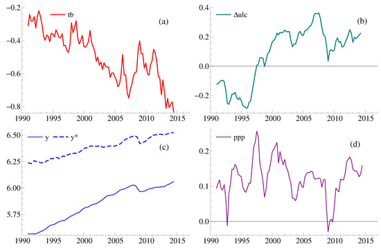
Figure 1.
Data. (a) is the trade balance between the UK and Germany; (b) is the unit labour cost differential between the UK and Germany; (c) and are the logs of the UK and German gross domestic products, respectively; (d) is the terms of trade.
In this empirical illustration, we analyse the data using a bivariate partial autoregressive model for and , with , and assumed to be weakly exogenous for the class of parameters of interest such as cointegrating vectors; that is, and . This assumption is based on Schreiber’s study, suggesting that modelling the bilateral trade block centering on and appears to be conformable to the underlying data structure. The lag-length is selected for our bivariate partial autoregressive model.
With regard to the issue on a structural break, we adopt a broken trend specification; that is, the presence of a shift in the restricted trend as well as the unrestricted constant. The second sub-sample period starts in , corresponding to the observation point in for , which results in the selection of relative break points and . According to (10), our bivariate model with requires a set of two impulse dummy variables for the initial values of the second sub-sample periods. In addition, a pair of impulse dummy variables, and , is employed in our model to capture outliers in the data, as in Schreiber (2015); the former variable is 1 in 1998.1 and zero otherwise for an outlier due to the Asian financial crisis, while the latter is 1 in 2006.2 and zero otherwise, corresponding to an outlier attributable to an increase in oil prices.
A set of residual diagnostic tests for the partial system is reported in Table 3. Most of the test statistics are given in the form F(), which denotes an approximate F test (with relevant degrees of freedom and ) against the alternative hypothesis j. The alternative hypotheses are specified as: 5th-order serial correlation (F, Godfrey 1978), 4th-order autoregressive conditional heteroscedasticity (F, Engle 1982), heteroscedasticity (F, White 1980). Chi-squared tests for normality (, Doornik and Hansen 2008) are also recorded in the table. We also note the following caveats based on recent advances in the field of mis-specification tests: Nielsen (2006) demonstrated that F is a valid test in the presence of unit roots; Berenguer-Rico and Wilms (2018) showed that F is valid after eliminating outliers from the observations, while is not necessarily valid after the removal of outliers, which was demonstrated by Berenguer-Rico and Nielsen (2017). In any case, no evidence is found in Table 3, suggesting significant mis-specification problems. We can thus judge this partial system is formulated sufficiently well to be subjected to tests for cointegrating rank.
Table 3.
Diagnostic test statistics for the estimated partial system.
Table 4 presents a class of test statistics for the determination of cointegrating rank, along with the corresponding p-values and approximate 95% limit quantiles calculated from the response surface outcomes in the previous section. We used Table A1 in Appendix A to calculate approximates to , and , and then applied them to the mappings (29) and (30) adjusted for extra terms, so that the gamma-distribution approximation method yielded the p-values. Table 4 shows that, at the 5% level, the null hypothesis is rejected while the hypothesis fails to be rejected. Hence, this formal analysis enables us to reach the conclusion of , which supports the informal analysis of Schreiber (2015).
Table 4.
Testing for cointegrating rank.
The estimated cointegrating relationship under some additional restrictions is
where a figure in brackets under each coefficient is a standard error and is a stationary error. The signs of the coefficients in (35) are the same as those in Schreiber (2015)’s cointegrating equation except for . The German income was insignificant in her cointegrating relationship and thus removed from it, while, in (35), plays a significant role, along with . As a result of checking a set of unrestricted estimates for the cointegrating vector, we have arrived at Equation (35), where the coefficients of and are restricted to add to zero, while a zero-restriction is placed on the coefficient for ; that is, a linear trend is present only in the second sub-sample period. The test statistic for these restrictions is , in which the figure in square brackets is a p-value according to . Thus, the hypothesis of the overall restrictions cannot be rejected at the 5% level.
There are several interesting aspects of Equation (35) that are worth discussing here. The real income difference between Germany and the UK, , has a positive coefficient, implying that a spread in the income difference leads to an improvement in the UK trade balance with Germany. This finding is interpretable in the context of an income effect from each of the two countries. The coefficient for the terms of trade, should also be noted. It is negative, thus indicating a relative price effect on the trade balance in a theory-consistent manner; that is, a decrease in exports prices relative to import prices leads to trade balance improvement, so that the well-known elasticity approach to trade balance appears to be empirically valid for the two countries. Furthermore, the linear trend t is significant solely in the second sub-sample period, suggesting long-lasting influences of the global recession on the two countries’ trade balance and other economic variables.
Finally, we will check that the three variables, , and , are indeed weakly exogenous for the class of parameters of interest. We follow the testing procedure suggested by Johansen (1992a), Boswijk (1992) and HJNR. First, the restricted cointegrating combination is added as a regressor to a marginal system (9) for . Second, a standard regression analysis is performed to test for the significance of the cointegrating combination in each equation. Table 5 reports a class of test statistics for the exclusion of the empirical cointegrating linkage from each equation in the marginal system. Judging from the reported p-values according to , none of the test statistics indicate evidence against the assumption of weak exogeneity; thus, the preceding partial-system analysis of cointegrating rank has been justified.
Table 5.
Checking weak exogeneity.
6. Conclusions
This study has explored partial cointegrated vector autoregressive models subject to structural breaks in deterministic terms, a linear trend and constant. The Granger–Johansen representation of the full model in JMN has been reexamined, leading to a useful clarification of roles of the initial values in asymptotic analysis. A class of log likelihood ratio test statistics for cointegrating rank has then been introduced in the proposed partial-model framework. We have investigated asymptotic theory under a general class of innovation distributions allowing martingale difference sequences with conditional heteroscedasticity. The derived limit distributions of the statistics are closely related to those for the full models investigated by JMN. This relationship allows us to perform a response surface analysis in a simplified full-system framework, instead of relying on laborious partial-system-based simulations. The outcomes of the analysis are summarised as a set of two statistical tables providing valuable information for inference on the underlying cointegrating rank. Lastly, an empirical analysis of real-life data from the UK and Germany has demonstrated the practicality of these tables in applied economic research. As a result of this study, the partial cointegrated models have become more flexible and reliable devices for modelling time series data subject to various structural breaks.
Recently, bootstrap methods have been proposed for cointegration rank testing in full systems (Cavaliere et al. 2012). It would be interesting to extend those to partial systems with or without breaks.
Supplementary Materials
The following are available online at https://www.mdpi.com/2225-1146/7/4/42/s1: A preadsheet for implementing the response surface in Table A1 and Table A2, as well as an Ox program for simulating the asymptotic distributions.
Author Contributions
The authors made equal contributions.
Funding
T. Kurita gratefully acknowledges financial support for this work from JSPS KAKENHI (Grant Nos: 15KK0141 and 26380349).
Acknowledgments
We are grateful to the editors and two anonymous referees for constructive comments. The results reported in this paper were presented at Norwegian University of Science and Technology (NTNU), Statistics Norway and the University of Copenhagen. We would like to thank Gunnar Bårdsen, Pål Boug, Søren Johansen and various other seminar participants for helpful comments and suggestions.
Conflicts of Interest
The authors declare no conflict of interest.
Appendix A. Tables for Response Surfaces
Table A1.
Response surfaces for broken trend models.
Table A1.
Response surfaces for broken trend models.
| const. | 4.14 | const. | 0.5987 | const. | −1.298 |
| −6.301 | −0.0538 | 0.03616 | |||
| 5.8842 | a | −1.039 | −0.027 | ||
| −2.32576 | b | −0.39 | −2.022 | ||
| 0.17 | 0.00686 | a | −8.689 | ||
| a | 2.6165 | 5.547 | b | 2.225 | |
| b | 2.5245 | 2.331 | 59.77 | ||
| −0.0572 | 1.841 | 24.31 | |||
| −0.0971 | −0.00033 | −5.156 | |||
| −7.550 | −10.42 | −133.5 | |||
| −5.323 | −4.325 | −59.05 | |||
| −7.412 | −2.553 | −29.55 | |||
| −0.000124 | 9.905 | −66.58 | |||
| 0.161 | 1.862 | 255.3 | |||
| 0.179 | −61.09 | 280.5 | |||
| 10.40 | −17.09 | 155.3 | |||
| 6.096 | −11.48 | −240 | |||
| 5.851 | 117.68 | 21.32 | |||
| −8.860 | 35.19 | 71.68 | |||
| −4.948 | 18.6 | −305.7 | |||
| 46.15 | −8.836 | −321.1 | |||
| 31.85 | 1.033 | 332.1 | |||
| 26.12 | 66.94 | 0.038 | |||
| −86.58 | 10.84 | −0.184 | |||
| −50.50 | −140.88 | ||||
| −28.78 | −30.16 | ||||
| 5.296 | −10.05 | ||||
| 2.386 | 2.107 | ||||
| −29.03 | −1.029 | ||||
| −19.46 | −20.63 | ||||
| −13.42 | 3.511 | ||||
| 62.00 | 45.85 | ||||
| −5.880 | 4.267 | ||||
| 34.59 | 0.062 | ||||
| 15.93 |
Note: is 1 when and zero otherwise.
Table A2.
Response surfaces for broken constant models.
Table A2.
Response surfaces for broken constant models.
| const. | 4.95486 | const. | 0.4472 | const. | −1.531 |
| −9.263 | 1.17564 | 0.9029 | |||
| 9.162 | −1.5294 | a | 4.164 | ||
| −3.662 | b | 0.8286 | 0.01579 | ||
| a | 3.05 | −0.0646 | 0.3388 | ||
| b | 0.3315 | 1.75 | −27.16 | ||
| 0.01738 | 0.04051 | −14.15 | |||
| −0.128 | −2.084 | −0.0013 | |||
| −14.61 | −3.698 | −0.0167 | |||
| −4.14 | −0.788 | −19.65 | |||
| −2.419 | −4.819 | 14.03 | |||
| −0.00084 | −3.897 | 42.2 | |||
| 0.3264 | 30.49 | 17.43 | |||
| 0.1302 | −5.108 | −77.72 | |||
| 0.0266 | 2.273 | −20.52 | |||
| 21.56 | −40.9 | 278.7 | |||
| 5.56 | 13.37 | 313.6 | |||
| 3.03 | 16 | 169.1 | |||
| −5.742 | 3.795 | −461.7 | |||
| 3.339 | −110.5 | −562.9 | |||
| 44.2 | 184.8 | −221.2 | |||
| 9.66 | −4.478 | 81.64 | |||
| −4.44 | 0.5014 | −315 | |||
| −81.67 | −9.833 | −384.8 | |||
| −15.2 | 73.02 | −114.6 | |||
| 2.41 | −5.835 | 804 | |||
| −3.44 | −130.2 | −290 | |||
| −24.23 | 4.743 | 860.7 | |||
| 9.6 | −0.2472 | 205.2 | |||
| 47.34 | 0.06919 | 0.18 | |||
| −7.22 | 3.765 | −0.00017 | |||
| −0.884 | 1.337 | ||||
| −14.06 | −0.0215 | ||||
| 1.944 | −0.408 |
Note: is 1 when and zero otherwise.
Appendix B. Proof of the Granger–Johansen Representation
This section provides a proof of Theorem 1, in which the Granger–Johansen representation of the full model with deterministic breaks is presented.
Proof of Theorem 1.
The companion form of the homogenous Equation (13) is
on the effective sample, see (7). As shown by Hansen (2005, Lemma A.1), stated in Assumption 1 implies that the above homogenous equation is an system satisfying
which is a stable equation (Lai and Wei 1985).
We then follow Kurita and Nielsen (2009) in the analysis of non-stationary components. Start by the homogenous Equation (13) for and :
Pre-multiplying the above equation by and replacing , we collect repeated terms on the left-hand side to find
by recalling . Summing over yields
Apply the orthogonal projection identity to the left-hand side and then pre-multiply both sides by to find the C matrix. Shifting to the right hand side, we arrive at
Adding on both sides results in
Using the notation for as well as the matrix defined in (14) leads to the first desired result (17).
Appendix C. Proofs of Asymptotic Results
In this section, we present a high-level assumption which overrides Assumptions 2 and 3 in the subsequent arguments. We then provide some specific lemmas required for proofs of the limit theorems in Section 3. Finally, we proceed to the proofs of Theorems 2 and 3.
We introduce some notation. For a vector v, let the outer product be . For a matrix m, the spectral norm is Note that
Appendix C.1. A High Level Assumption
In order to give proofs of the theorems introduced in this paper, we need a Law of Large Numbers for the approximately stationary components of the full model, while we require a Functional Central Limit Theorem and a convergence to a stochastic integral for the non-stationary components of the full model. We formulate these as a the following high level assumption and then prove that it is satisfied under Assumptions 1 and 2.
Assumption A1.
Let be a p-dimensional random variables and suppose that Assumption 1 is satisfied. Let satisfy the homogenous Equation (13) and define as
Suppose that
and
where Ω and are positive definite matrices. Furthermore, let be a p-dimensional Brownian motion with variance Ω. Suppose that, for ,
as a process on endowed with the Skorokhod metric with common distortion. Finally,
The next result explores the conditions of Brown (1971). Subsequently, we use this to show that Assumptions 1 and 2 imply Assumption A1.
Lemma A1.
Suppose Assumption 2 is satisfied. Then,
- (a)
- ;
- (b)
- for all ;
- (c)
- for all ;
- (d)
Proof of Lemma A1.
( Brown (1971, Lemma 2) shows that the conditional Lindeberg condition and the marginal Lindeberg condition are equivalent under Assumption 2
First, suppose Assumption 2, so that as . Thus, , and , it follows that
Thus, given and for , we find
so that the conditional Lindeberg condition follows.
Second, suppose Assumption 2, so that Chebychev’s inequality gives
Next, by the Cauchy–Schwarz inequality and Assumption 2 we get
Hence, so that the marginal Lindeberg condition holds.
We define and and show that Since is symmetric, the spectral norm equals the spectral radius, thus it suffices to show that vanishes for any linear combination v. In turn, it suffices to consider univariate martingale difference sequences
First, suppose Assumption 2 holds, so that as . We follow an argument inspired by Anderson and Kunitomo (1992, Theorem 2). Hall and Heyde (1980, Theorem 2.23) show that whenever the Lindeberg condition in part holds and as To prove the tightness condition, note that
Thus, to analyse the tightness probability bound,
This bound is uniform in T so that which vanishes by Assumption 2
Second, suppose Assumption 2 holds, so that Let The Chebychev inequality and the uncorrelatedness of martingale differences gives
Jensen’s inequality shows Thus, the inequality shows that Thus,
We show for all Note that Boole’s inequality gives On the set , we get the further bound which vanishes by part . □
We then prove that Assumption A1 is satisfied under Assumptions 1 and 2.
Lemma A2.
Suppose that and satisfy Assumptions 1 and 2, respectively, while solves the homogenous Equation (13). Then, Assumption A1 is satisfied.
Proof of Lemma A2.
Note that the process equals , which is studied in Theorem 1. It satisfies Equation (16), which is of the form with for and , where has spectral radius less than unity as verified in Theorem 1.
For (A3), we apply Anderson and Kunitomo (1992, Lemma 1). This requires that which is proved in Lemma A1 using Assumption 2.
For (A4), use Assumption 2 We apply Lemma 2 in Anderson and Kunitomo (1992) to show the convergence of the product moment matrix, which requires Assumption 2. Assumption 2 states that is a positive definite matrix, which results in the positive definiteness of by Anderson and Kunitomo (1992, Lemma 3).
For (A4) using Assumption 2 We follow Anderson and Kunitomo (1992, Lemma 2) but avoid their truncation argument. We first argue that Since is a martingale difference sequence with second moments due to Assumption 2 and the spectral norm is bounded by the trace, we obtain
Applying iterated expectations and using that is bounded by Assumption 2 gives . Noting that and using that is a martingale difference array, we arrive at
Using that is bounded and has spectral radius less than unity,
As a consequence and, by the Markov inequality, Next, we show in probability. Since , then
Here, the second term converges to by Assumption 2 while the last two terms vanish. Since , we therefore get
This is a linear equation in so that in probability where solves Anderson and Kunitomo (1992, Lemma 3) show invertibility of .
For (A5), the Functional Central Limit Theorem follows from the univariate result of Brown (1971, Theorem 3), equipped with Cramér–Wold device, see Billingsley (1968, Theorem 7.7). Brown’s result applies under Assumption 2 and either of the Lindeberg condition established in Lemma A1 under Assumption 2. When using Brown’s result, it is convenient to define the univariate variables and . Brown is concerned with the continuously embedded random walk through the points , while we are concerned with the right continuous random walk that is constant on the half-open intervals . The two embeddings reconcile since for some constant by Assumption 2 and since vanishes by Lemma A1 under Assumption 2.
For (A6), the convergence to a stochastic integral for the univariate case is based on the results of Jakubowski et al. (1989), which was referred to by Kurtz and Protter (1996), while the convergence to a stochastic integral for the multivariate case is based on the results of Kurtz and Protter (1991). For the univariate case, Kurtz and Protter (1996, Theorem 7.1) show that we need to check that the martingale array is uniformly tight, as required by Jakubowski et al. (1989) or, equivalently, it has uniformly controlled variations. We use Kurtz and Protter (1991, Theorem 2.2), which applies to the multivariate case; see also Hansen (1992, Theorem 2.1). Choose so that in Kurtz and Protter’s notation. For each , , choose stopping times so that Then, we obtain a quadratic variation processes
so that . From Assumption 2, it follows that Consequently, we have . In turn, for each t, so that has uniformly controlled variations. □
Proof of Lemma 1.
Assumption 3 has , so that follows and Assumption 2 holds. Taking iterated expectations, we obtain , which leads to and thus Assumption 2 is satisfied. Lastly, we show that Assumption 2 is implied by Assumption 3. Using Hölder’s inequality, we find, for ,
in which we note the equality . Hence, writing the expectation of the indicator as a probability, and also using Markov’s inequality, we arrive at
In combination, we obtain , which vanishes as uniformly in t, since the is uniformly bounded by assumption. □
Remark A1.
We give an example of a martingale difference sequence satisfying but violating Assumption 2, i.e., in probability, which is from Anderson and Kunitomo (1992). Consider the probability space , where is the Borel field on and is the uniform distribution. Consider also a dyadic sequence with indices and , so that , and define
We note that while is uniformly bounded in The natural filtration of is then given by the σ-fields and so on. We find that while for all a and all so that the random variables cannot vanish in probability.
Appendix C.2. Several Lemmas for the Partial Systems
The asymptotic properties of the product moment matrices, for defined in (24), are investigated so as to adapt Lemmas 10.1 and 10.3 of Johansen (1995) to the present model. We do this by combining various ideas and techniques from HJNR, JMN and Kurita and Nielsen (2009). These papers assume normal innovations, which we have generalised as Assumptions 2 and 3 in our study. This means that we have to be careful when defining the limits of product moments of various non-integrated components. This issue is addressed in the following lemma:
Lemma A3.
Suppose that Assumptions 1 and A1 are satisfied. Let
Let be relative break points for and define the sample product moment matrix of corrected for and a constant as
Then, as with fixed relative break points , we get that converges in probability to a positive definite matrix with the structure
where and hold.
Proof of Lemma A3.
We start with the homogenous Equation (16). For and , this equation can always be solved as
and, in the first sub-sample period or , the initial value can be treated as fixed, so that the process for becomes uniformly bounded in probability by noting that it equals in Assumption A1. Similarly, by iterating over all the other start-up values, the process for and is also uniformly bounded in probability. Since the number of breaks is finite, is uniformly bounded in probability jointly for .
Since is uniformly bounded in probability, it follows that is also uniformly bounded in probability. Note that is identical throughout all sub-sample periods. The intercepts and are eliminated from and respectively, when demeaning them within each sub-sample period. Consequently, we can apply the Law of Large Numbers (A4) in Assumption A1 to
which, for , converges in probability to a positive definite matrix denoted as
for by Assumption A1. Since both and consist of the past values of , it follows from (A4) that and hold. Note that the model equation is
for We can derive three properties from this equation. First, we post-multiply (A9) by and then exploit and to find which is the first property. The next one is
where the left-hand side is the limit of the sample regression coefficient for regressed on , and an intercept. This property is demonstrated by substituting from (A9) into ; we then arrive at the limit result
from which (A10) follows by noting that and . The third property is
The left-hand side of (A11) is the limit of the sample product moment of regressed on , and an intercept, due to and . The right-hand side of (A11) is the limit of the sample product moment of regressed on , and an intercept, where we have exploited the identity (A10).
Now, we return to (A8) and partial out to obtain
for which we have that while and Thus, (A12) is reduced to
where
Furthermore, noting and , we define
for and . The use of Slutsky’s theorem then leads to (A7).
It is left to show that and For the first expression, we apply the identities in (A13) to (A10) so as to obtain
Taking partitioned inversion in (A14) results in For the second expression, we apply the identities in (A13) to (A11) to find
Inserting (A14) into (A15) and taking its partitioned inversion, we arrive at
by noting from (A14) that holds. □
Recalling the decomposition , we find the following equivalence in the lower-right submatrix of (A7) in Lemma A3:
Under the normality assumption for as in HJNR, we could form the conditional variance of the two elements and given the element Moving away from normality under Assumptions 2 and 3, we need to consider instead the limit of a product moment matrix consisting of linear combinations of these elements, defined in the following manner:
which appears in (A17) in Lemma A6, and where
Let us recall the weak exogeneity condition , which implies
Finally, recall from (4) that the limit variance of innovations in the partial equation equals under Assumption A1. Within each sub-sample period, the setup here is identical to that of HJNR. We therefore obtain the following equation, which adapts Equation (10).6 in Johansen (1995, Lemma 10.1).
Lemma A4
(HJNR, Lemma 4). Suppose that Assumptions 1 and A1 are satisfied under . Then,
We now explore the limit of the common trends within each sub-sample period. Define
and the next lemma is a combination of Lemma A.1 in JMN and Lemma 5 in HJNR.
Lemma A5.
Suppose that Assumptions 1 and A1 are satisfied. Consider the -dimensional process on endowed with the Skorokhod metric with common distortion across the dimensions. Let be a -dimensional Brownian motion with variance Ω for For and the process satisfies
The convergence holds jointly for and .
Proof of Lemma A5.
The Granger–Johansen representation (18) implies that, for and ,
Since has full row rank and is bounded in probability as shown in the proof of Lemma A3, the random walk component dominates . The initial value could be large when but it is eliminated when taking differences . Thus, the first element of converges to by the Functional Central Limit Theorem (A5) in Assumption A1. The second element also converges as desired since converges to u. As the number of breaks is finite, the convergence holds jointly for . □
Decompose , in which the dimensions of and are m and , respectively. Let us recall the notation , which was used in reduced rank regression in Section 3.1. The next lemma establishes the asymptotic theory for the product moment matrices for defined in (24).
Lemma A6.
Suppose that Assumptions 1 and A1 are satisfied under . Define , and
It then follows that
where
Proof of Lemma A6.
Recall the decomposition .
For (A17), we start with the left-hand side of (A12) and further partial out from the process, to which we then apply the Law of Large Numbers (A4) in Assumption A1. Follow the proof of Lemma A3 afterwards, supplemented with the definition of the limit expression (A16), in order to verify (A17).
For (A18), use Lemma A5, the continuous mapping theorem and Johansen (1995, Lemma 10.3).
For (A19), we note The Law of Large Numbers (A4) in Assumption A1 implies , in which is the demeaned version of as defined in (23). By (A3) and the Granger–Johansen representation in Theorem 1, we can replace with the demeaned version of The stochastic integral (A6) in Assumption A1 then gives (A19).
For (A20), we follow the strategy used for (A19); see also Johansen (1995, Lemma 10.3). □
Appendix C.3. Proofs of the Theorems in Section 3
Proof of Theorem 2.
Follow the proof of Theorem 11.1 in Johansen (1995) by using Lemmas A4 and A6 given above instead of his Lemmas 10.1 and 10.3, and also utilise invariance properties with respect to non-singular linear transformations as in the proof of Theorem 1 in HJNR. □
Proof of Theorem 3.
The proof presented here is based on Doornik (1998, §9). The asymptotic distribution of the test statistic in the partial model in Theorem 2 is rewritten as
The process for is a function of and , both of which are functions of the -dimensional standard Brownian motion Inspection of these functions shows that they are invariant to the relabelling of the coordinates of , so that are identically distributed and any pairs are also identically distributed. Hence,
In order to relate the moments of the limit distributions of the test statistics in the partial and full models, we evaluate the above expressions for in general and for For the means of the limit distributions, we find
Solving both equations for and equating the resulting expressions yield
For their variances, we obtain a set of equations similarly, which are solved for to find the desired expression. □
References
- Anderson, Theodore W., and Naoto Kunitomo. 1992. Asymptotic distributions of regression and autoregression coefficients with martingale difference disturbances. Journal of Multivariate Analysis 40: 221–43. [Google Scholar] [CrossRef]
- Bårdsen, Gunnar, Øyvind Eitrheim, Eilev S. Jansen, and Ragnar Nymoen. 2005. The Econometrics of Macroeconomic Modelling. Oxford: Oxford University Press. [Google Scholar]
- Berenguer-Rico, Vanessa, and Bent Nielsen. 2017. Marked and Weighted Empirical Processes of Residuals with Applications to Robust Regressions. Discussion Paper 841. Oxford: Department of Economics, University of Oxford. [Google Scholar]
- Berenguer-Rico, Vanessa, and Ines Wilms. 2018. White Heteroscedasticity Testing in Robust Regressions. Discussion Paper 853. Oxford: University of Oxford, Department of Economics. [Google Scholar]
- Billingsley, Patrick. 1968. Convergence of Probability Measures. New York: John Wiley & Sons. [Google Scholar]
- Boswijk, H. Peter. 1992. Cointegration, Identification and Exogeneity, 3rd ed. Tinbergen Institute Research Series; Amsterdam: Thesis Publishers, volume 37. [Google Scholar]
- Boswijk, H. Peter. 1995. Efficient inference on cointegration parameters in structural error correction models. Journal of Econometrics 69: 133–58. [Google Scholar] [CrossRef]
- Boswijk, H. Peter, Giuseppe Cavaliere, Anders Rahbek, and A. M. Robert Taylor. 2016. Inference on co-integration parameters in heteroskedastic vector autoregressions. Journal of Econometrics 192: 64–85. [Google Scholar] [CrossRef]
- Boswijk, H. Peter, and Jurgen A. Doornik. 2005. Distribution approximations for cointegration tests with stationary exogenous regressors. Journal of Applied Econometrics 20: 797–810. [Google Scholar] [CrossRef]
- Brown, B. M. 1971. Martingale central limit theorems. Annals of Mathematical Statistics 42: 59–66. [Google Scholar] [CrossRef]
- Cavaliere, Giuseppe, Luca De Angelis, and Luca Fanelli. 2018. Co-integration rank determination in partial systems using information criteria. Oxford Bulletin of Economics and Statistics 80: 65–89. [Google Scholar] [CrossRef]
- Cavaliere, Giuseppe, Anders Rahbek, and A. M. Robert Taylor. 2010. Cointegration rank testing under conditional heteroskedasticity. Econometric Theory 26: 1719–60. [Google Scholar] [CrossRef]
- Cavaliere, Giuseppe, Anders Rahbek, and A. M. Robert Taylor. 2012. Bootstrap determination of the co-integration rank in vector autoregressive models. Econometrica 80: 1721–40. [Google Scholar]
- Chan, Ngai Hang, and Ching Zong Wei. 1988. Limiting distributions of least squares estimates of unstable autoregressive processes. Annals of Statistics 16: 367–401. [Google Scholar] [CrossRef]
- Doornik, Jurgen A. 1998. Approximations to the asymptotic distribution of cointegration tests. Journal of Economic Surveys 12: 573–93. [Google Scholar] [CrossRef]
- Doornik, Jurgen A. 2003. Asymptotic Tables for cointegration Tests Based on the GAmma-Distribution Approximation. Available online: www.doornik.com/research/coigamma_tables.pdf (accessed on 4 October 2019).
- Doornik, Jurgen A. 2013. An Object-Oriented Matrix Programming Language—OX7. London: Timberlake. [Google Scholar]
- Doornik, Jurgen A., and Henrik Hansen. 2008. An omnibus test for univariate and multivariate normality. Oxford Bulletin of Economics and Statistics 70: 927–39. [Google Scholar] [CrossRef]
- Doornik, Jurgen A., and David F. Hendry. 2013. PcGive 14. London: Timberlake, volume 2. [Google Scholar]
- Doornik, Jurgen A., David F. Hendry, and Bent Nielsen. 1998. Inference in cointegrating models: UK M1 revisited. Journal of Economic Surveys 12: 533–72. [Google Scholar] [CrossRef]
- Engle, Robert F. 1982. Autoregressive conditional heteroscedasticity with estimates of the variance of united kingdom inflation. Econometrica 50: 987–1108. [Google Scholar] [CrossRef]
- Engle, Robert F., David F. Hendry, and Jean-Francois Richard. 1983. Exogeneity. Econometrica 51: 277–304. [Google Scholar] [CrossRef]
- Ericsson, Neil R., and James G. MacKinnon. 2002. Distributions of error correction tests for cointegration. Econometrics Journal 5: 285–318. [Google Scholar] [CrossRef]
- Godfrey, Leslie G. 1978. Testing against general autoregressive and moving average error models when the regressors include lagged dependent variables. Econometrica 46: 1293–301. [Google Scholar] [CrossRef]
- Hall, P., and C. C. Heyde. 1980. Martingale Limit Theory and Its Applications. San Diego: Academic Press. [Google Scholar]
- Hannan, E. J., and C. C. Heyde. 1972. On limit theorems for quadratic functions of discrete time series. Annals of Mathematical Statistics 43: 2058–66. [Google Scholar] [CrossRef]
- Hansen, Bruce E. 1992. Convergence to stochastic integrals for dependent heterogeneous processes. Econometric Theory 8: 489–500. [Google Scholar] [CrossRef]
- Hansen, Peter Reinhard. 2005. Granger’s representation theorem: A closed-form expression for I(1) processes. Econometrics Journal 8: 23–38. [Google Scholar]
- Harbo, Ingrid, Søren Johansen, Bent Nielsen, and Anders Rahbek. 1998. Asymptotic inference on cointegrating rank in partial systems. Journal of Business and Economic Statistics 16: 388–99. [Google Scholar]
- Harvey, Andrew, and Stephen Thiele. 2017. Co-Integration and Control: Assessing the Impact of Events Using Time Series Data. Working Paper 1731. Cambridge: University of Cambridge, Faculty of Economics. [Google Scholar]
- Hendry, David F., and Michael Massmann. 2007. Co-breaking: Recent advances and a synopsis of the literature. Journal of Business & Economic Statistics 25: 33–51. [Google Scholar]
- Inoue, Atsushi. 1999. Tests of cointegrating rank with a trend-break. Journal of Econometrics 90: 215–37. [Google Scholar] [CrossRef]
- Jakubowski, Adam, Jean Ménin, and Gilles Pages. 1989. Convergence en loi des suites d’integrales stochastiques sur l’espace D1 de skorokhod. Probability Theory and Related Fields 81: 111–37. [Google Scholar] [CrossRef]
- Johansen, Søren. 1988. Statistical analysis of cointegration vectors. Journal of Economic Dynamics & Control 12: 231–54. [Google Scholar]
- Johansen, Søren. 1992a. Cointegration in partial systems and the efficiency of single-equation analysis. Journal of Econometrics 52: 389–402. [Google Scholar] [CrossRef]
- Johansen, Søren. 1992b. Testing weak exogeneity and the order of cointegration in the UK money demand data. Journal of Policy Modeling 14: 313–34. [Google Scholar] [CrossRef]
- Johansen, Søren. 1995. Likelihood Based Inference on Cointegration in the Vector Autoregressive Model. Oxford: Oxford University Press. [Google Scholar]
- Johansen, Søren, Rocco Mosconi, and Bent Nielsen. 2000. Cointegration analysis in the presence of structural breaks in the deterministic trend. Econometrics Journal 3: 216–49. [Google Scholar] [CrossRef]
- Juselius, Katarina. 2006. The Cointegrated VAR Model. Oxford: Oxford University Press. [Google Scholar]
- Kurita, Takamitsu. 2011. Local power of likelihood-based tests for cointegrating rank: Comparative analysis of full and partial systems. Journal of Time Series Analysis 32: 672–79. [Google Scholar] [CrossRef]
- Kurita, Takamitsu, and Bent Nielsen. 2009. Cointegrated vector autoregressive models with adjusted short-run dynamics. Quantitative and Qualitative Analysis in Social Sciences 3: 43–77. [Google Scholar]
- Kurita, Takamitsu, Heino Bohn Nielsen, and Anders Rahbek. 2011. An I(2) cointegration model with piecewise linear trends. Econometrics Journal 14: 131–55. [Google Scholar] [CrossRef]
- Kurtz, Thomas G., and Philip E. Protter. 1991. Weak limit theorems for stochastic integrals and stochastic differential equations. Annals of Probability 19: 1035–70. [Google Scholar] [CrossRef]
- Kurtz, Thomas G., and Philip E. Protter. 1996. Weak convergence of stochastic integrals and differential equations. In Probabilistic Models for Nonlinear Partial Differential Equations. Edited by Denis Talay and Luciano Tubaro. Lecture Notes in Mathematics; Berlin: Springer, volume 1627, pp. 197–285. [Google Scholar]
- Lai, Tze Leung, and Ching Zong Wei. 1982. Least squares estimates in stochastic regression models with applications to identification and control of dynamic systems. Annals of Statistics 10: 154–66. [Google Scholar] [CrossRef]
- Lai, T. L., and C. Z. Wei. 1985. Asymptotic properties of multivariate weighted sums with applications to stochastic regression in linear dynamic systems. In Multivariate Analysis—VI. Edited by P. R. Krishnaiah. Amsterdam: Elsevier, pp. 375–93. [Google Scholar]
- MacKinnon, James G., Alfred A. Haug, and Leo Michelis. 1999. Numerical distributions of likelihood ratio tests of cointegration. Journal of Applied Econometrics 14: 563–77. [Google Scholar] [CrossRef]
- Nielsen, B. 1997. Bartlett correction of the unit root test in autoregressive models. Biometrika 84: 500–4. [Google Scholar] [CrossRef]
- Nielsen, Bent. 2005. Strong consistency results for least squares estimators in general vector autoregressions with deterministic terms. Econometric Theory 21: 534–61. [Google Scholar] [CrossRef]
- Nielsen, Bent. 2006. Order determination in general vector autoregressions. In Time Series and Related Topics: In Memory of Ching-Zong Wei. Edited by Hwai-Chung Ho, Ching-Kang Ing and Tze Leung Lai. Lecture Notes–Monograph Series. Beachwood: Institute of Mathematical Statistics, vol. 52, pp. 93–112. [Google Scholar]
- Paruolo, Paolo. 1997. Asymptotic inference on the moving average impact matrix in cointegrated I(1) var systems. Econometric Theory 13: 79–118. [Google Scholar] [CrossRef]
- Paruolo, Paolo, and Anders Rahbek. 1999. Weak exogeneity in I(2) VAR systems. Journal of Econometrics 93: 281–308. [Google Scholar] [CrossRef]
- Perron, Pierre. 1989. The great crash, the oil price shock, and the unit root hypothesis. Econometrica 57: 1361–401, Erratum in volume 61, 248–49. [Google Scholar] [CrossRef]
- Pesaran, M. Hashem, Yongcheol Shin, and Richard J. Smith. 2000. Structural analysis of vector error correction models with exogenous I(1) variables. Journal of Econometrics 97: 293–343. [Google Scholar] [CrossRef]
- Rahbek, Anders, and Rocco Mosconi. 1999. Cointegration rank inference with stationary regressors in VAR models. Econometrics Journal 2: 76–91. [Google Scholar] [CrossRef]
- Schreiber, Vanessa. 2015. Cointegration Analysis of the Exchange Rate and Bilateral Trade between the United Kingdom and Germany. M.Phil. thesis, University of Oxford, Oxford, UK. [Google Scholar]
- Seo, Byeongseon. 1998. Statistical inference on cointegration rank in error correction models with stationary covariates. Journal of Econometrics 85: 339–85. [Google Scholar] [CrossRef]
- White, Halbert. 1980. A heteroskedasticity-consistent covariance matrix estimator and a direct test for heteroskedasticity. Econometrica 48: 817–38. [Google Scholar] [CrossRef]
© 2019 by the authors. Licensee MDPI, Basel, Switzerland. This article is an open access article distributed under the terms and conditions of the Creative Commons Attribution (CC BY) license (http://creativecommons.org/licenses/by/4.0/).