Measures of Dispersion and Serial Dependence in Categorical Time Series

Abstract

The analysis and modeling of categorical time series requires quantifying the extent of dispersion and serial dependence. The dispersion of categorical data is commonly measured by Gini index or entropy, but also the recently proposed extropy measure can be used for this purpose. Regarding signed serial dependence in categorical time series, we consider three types of $\kappa$-measures. By analyzing bias properties, it is shown that always one of the $\kappa$-measures is related to one of the above-mentioned dispersion measures. For doing statistical inference based on the sample versions of these dispersion and dependence measures, knowledge on their distribution is required. Therefore, we study the asymptotic distributions and bias corrections of the considered dispersion and dependence measures, and we investigate the finite-sample performance of the resulting asymptotic approximations with simulations. The application of the measures is illustrated with real-data examples from politics, economics and biology.

1. Introduction

In many applications, the available data are not of quantitative nature (e.g., real numbers or counts) but consist of observations from a given finite set of categories. In the present article, we are concerned with data about political goals in Germany, fear states in the stock market, and phrases in a bird’s song. For stochastic modeling, we use a categorical random variable X, i.e. a qualitative random variable taking one of a finite number of categories, e.g. $m+1$ categories with some $m\in \mathbb{N}$. If these categories are unordered, X is said to be a nominal random variable, whereas an ordinal random variable requires a natural order of the categories (Agresti 2002). To simplify notations, we always assume the possible outcomes to be arranged in a certain order (either lexicographical or natural order), i.e. we denote the range (state space) as $\mathcal{S}=\{s_0,s_1,\dots ,s_m\}$. The stochastic properties of X can be determined based on the vector of marginal probabilities by $\mathit{p}={(p_0,\dots ,p_m)}^{\top }\in {[0;1]}^{m+1}$, where $p_i=P(X=s_i)$ (probability mass function, PMF). We abbreviate $s_k\left(\mathit{p}\right):={\sum }_{j=0}^m{p}_j^k$ for $k\in \mathbb{N}$, where $s_1\left(\mathit{p}\right)=1$ has to hold. The subscripts “$0,1,\dots ,m$” are used for $\mathcal{S}$ and p to emphasize that only m of the probabilities can be freely chosen because of the constraint $p_0=1-p_1-\dots -p_m$.

Well-established dispersion measures for quantitative data, such as variance or inter quartile range, cannot be applied to qualitative data. For a categorical random variable X, one commonly defines dispersion with respect to the uncertainty in predicting the outcome of X(Kvålseth 2011b; Rao 1982; Weiß and Göb 2008). This uncertainty is maximal for a uniform distribution ${\mathit{p}}_{\mathrm{uni}}={(\frac{1}{m+1},\dots ,\frac{1}{m+1})}^{\top }$ on $\mathcal{S}$ (a reasonable prediction is impossible if all states are equally probable, thus maximal dispersion), whereas it is minimal for a one-point distribution ${\mathit{p}}_{\mathrm{one}}$ (i.e., all probability mass concentrates on one category, so a perfect prediction is possible). Obviously, categorical dispersion is just the opposite concept to the concentration of a categorical distribution. To measure the dispersion of the categorical random variable X, the most common approach is to use either the (normalized) Gini index (also index of qualitative variation, IQV) (Kvålseth 1995; Rao 1982) defined as

$${\nu }_{\mathrm{G}}=\frac{m+1}{m}\left(1-s_2\left(\mathit{p}\right)\right),$$

(1)

or the (normalized) entropy (Blyth 1959; Shannon 1948) given by

$${\nu }_{\mathrm{En}}=\frac{-1}{ln(m+1)}{\sum }_{i=0}^m{p}_{i}ln{p}_i\mathrm{with}0·ln0:=0.$$

(2)

Both measures are minimized by a one-point distribution ${\mathit{p}}_{\mathrm{one}}$ and maximized by the uniform distribution ${\mathit{p}}_{\mathrm{uni}}$ on $\mathcal{S}$. While nominal dispersion is always expressed with respect to these extreme cases, it has to be mentioned that there is an alternative scenario of maximal ordinal variation, namely the extreme two-point distribution; however, this is not further considered here.

If considering a (stationary) categorical process ${\left(X_t\right)}_{\mathbb{Z}}$ instead of a single random variable, then not only marginal properties are relevant but also information about the serial dependence structure (Weiß 2018). The (signed) autocorrelation function (ACF), as it is commonly applied in case of real-valued processes, cannot be used for categorical data. However, one may use a type of Cohen’s κ instead (Cohen 1960). A $\kappa$-measure of signed serial dependence in categorical time series is given by (see Weiß 2011, 2013; Weiß and Göb 2008);

$$\kappa \left(h\right)=\sum _{i=0}^m\frac{p_{ii}\left(h\right)-p_i^2}{1-s_2\left(\mathit{p}\right)}\in \left[\frac{-s_2\left(\mathit{p}\right)}{1-s_2\left(\mathit{p}\right)};1\right]\mathrm{for}\mathrm{lags}h\in \mathbb{N}.$$

(3)

Equation (3) is based on the lagged bivariate probabilities $p_{ij}\left(h\right)=P(X_t=i,X_{t-h}=j)$ for $i,j=0,\dots ,m$. $\kappa \left(h\right)=0$ for serial independence at lag h, and the strongest degree of positive (negative) dependence is indicated if all $p_{ii}\left(h\right)=p_i$ ($p_{ii}\left(h\right)=0$), i.e., if the event $X_{t-h}=s_i$ is necessarily followed by $X_t=s_i$ ($X_t\ne s_i$).

Motivated by a mobility index discussed by Shorrocks (1978), a simplified type of $\kappa$-measure, referred to as the modified κ, was defined by Weiß (2011, 2013):

$${\kappa }^{*}\left(h\right)=\frac{1}{m}\sum _{i=0}^m\frac{p_{ii}\left(h\right)-p_i^2}{p_i}\in \left[-\frac{1}{m};1\right]\mathrm{for}\mathrm{lags}h\in \mathbb{N}.$$

(4)

Except the fact that the lower bound of the range differs from the one in Equation (3) (note that this lower bound is free of distributional parameters), we have the same properties as stated before for $\kappa \left(h\right)$. The computation of ${\kappa }^{*}\left(h\right)$ is simplified compared to the one of $\kappa \left(h\right)$ and, in particular, its sample version ${\widehat{\kappa }}^{*}\left(h\right)$ has a more simple asymptotic normal distribution, see Section 5 for details. Unfortunately, ${\kappa }^{*}\left(h\right)$ is not defined if only one of the $p_i$ equals 0, whereas $\kappa \left(h\right)$ is well defined for any marginal distribution not being a one-point distribution. This issue may happen quite frequently for the sample version ${\widehat{\kappa }}^{*}\left(h\right)$ if the given time series is short (a possible circumvention is to replace all summands with $p_i=0$ by 0). For this reason, ${\kappa }^{*}\left(h\right),{\widehat{\kappa }}^{*}\left(h\right)$ appear to be of limited use for practice as a way of quantifying signed serial dependence. It should be noted that a similar “zero problem” happens with the entropy ${\nu }_{\mathrm{En}}$ in Equation (2), and, actually, we work out a further relation between ${\nu }_{\mathrm{En}}$ and ${\widehat{\kappa }}^{*}\left(h\right)$ below.

In the recent work by Lad et al. (2015), extropy was introduced as a complementary dual to the entropy. Its normalized version is given by

$${\nu }_{\mathrm{Ex}}=\frac{-1}{mln\left(\frac{m+1}{m}\right)}{\sum }_{i=0}^m(1-p_i)ln(1-p_i).$$

(5)

Here, the zero problem obviously only happens if one of the $p_i$ equals 1 (i.e., in the case of a one-point distribution). Similar to the Gini index in Equation (1) and the entropy in Equation (2), the extropy takes its minimal (maximal) value 0 (1) for $\mathit{p}={\mathit{p}}_{\mathrm{one}}$ ($\mathit{p}={\mathit{p}}_{\mathrm{uni}}$), thus also Equation (5) constitutes a normalized measure of nominal variation. In Section 2, we analyze its properties in comparison to Gini index and entropy. In particular, we focus on the respective sample versions ${\widehat{\nu }}_{\mathrm{Ex}}$, ${\widehat{\nu }}_{\mathrm{G}}$ and ${\widehat{\nu }}_{\mathrm{En}}$ (see Section 3). To be able to do statistical inference based on ${\widehat{\nu }}_{\mathrm{Ex}}$, ${\widehat{\nu }}_{\mathrm{G}}$ and ${\widehat{\nu }}_{\mathrm{En}}$, knowledge about their distribution is required. Up to now, only the asymptotic distribution of ${\widehat{\nu }}_{\mathrm{G}}$ and (to some part) of ${\widehat{\nu }}_{\mathrm{En}}$ has been derived; in Section 3, comprehensive results for all considered dispersion measures are provided. These asymptotic distributions are then used as approximations to the true sample distributions of ${\widehat{\nu }}_{\mathrm{Ex}}$, ${\widehat{\nu }}_{\mathrm{G}}$ and ${\widehat{\nu }}_{\mathrm{En}}$, which is further investigated with simulations and a real application (see Section 4).

The second part of this paper is dedicated to the analysis of serial dependence. As a novel competitor to the measures in Equations (3) and (4), a new type of modified $\kappa$ is proposed, namely

$${\kappa }^{\star }\left(h\right)=\sum _{i=0}^m\frac{p_{ii}\left(h\right)-p_i^2}{1-p_i}\in \left[\sum _{i=0}^m\frac{-p_i^2}{1-p_i};1\right]\mathrm{for}\mathrm{lags}h\in \mathbb{N}.$$

(6)

Again, this constitutes a measure of signed serial dependence, which shares the before-mentioned (in)dependence properties with $\kappa \left(h\right),{\kappa }^{*}\left(h\right)$. However, in contrast to ${\kappa }^{*}\left(h\right)$, the newly proposed ${\kappa }^{\star }\left(h\right)$ does not have a division-by-zero problem: except for the case of a one-point distribution, ${\kappa }^{\star }\left(h\right)$ is well defined. Note that, in Section 3.2, it turns out that ${\kappa }^{\star }\left(h\right)$ is related to ${\nu }_{\mathrm{Ex}}$ in some sense, e.g. $\kappa \left(h\right)$ is related to ${\nu }_{\mathrm{G}}$ and ${\kappa }^{*}\left(h\right)$ to ${\nu }_{\mathrm{En}}$. In Section 5, we analyze the sample version of ${\kappa }^{\star }\left(h\right)$ in comparison to those of $\kappa \left(h\right),{\kappa }^{*}\left(h\right)$, and we derive its asymptotic distribution under the null hypothesis of serial independence. This allows us to test for significant dependence in categorical time series. The performance of this ${\widehat{\kappa }}^{\star }$-test, in comparison to those based on $\widehat{\kappa },{\widehat{\kappa }}^{*}$, is analyzed in Section 6, where also two further real applications are presented. Finally, we conclude in Section 7.

2. Extropy, Entropy and Gini Index

As extropy, entropy and Gini index all serve for the same task, it is interesting to know their relations and differences. An important practical issue is the “$0ln0$”-problem, as mentioned above, which never occurs for the Gini index, only occurs in the case of a (deterministic) one-point distribution for the extropy, and always occurs for the entropy if only one $p_i=0$. Lad et al. (2015) further compared the non-normalized versions of extropy and entropy, and they showed that the first is never smaller than the latter. Actually, using the inequality $ln(1+x)>x/(1+x/2)$ for $x>0$ from Love (1980), it follows that

$$-{\sum }_{i=0}^m(1-p_i)ln(1-p_i)\ge -{\sum }_{i=0}^m{p}_{i}ln{p}_i\ge 1-s_2\left({p}\right),$$

(7)

(see Appendix B.1 for further details).

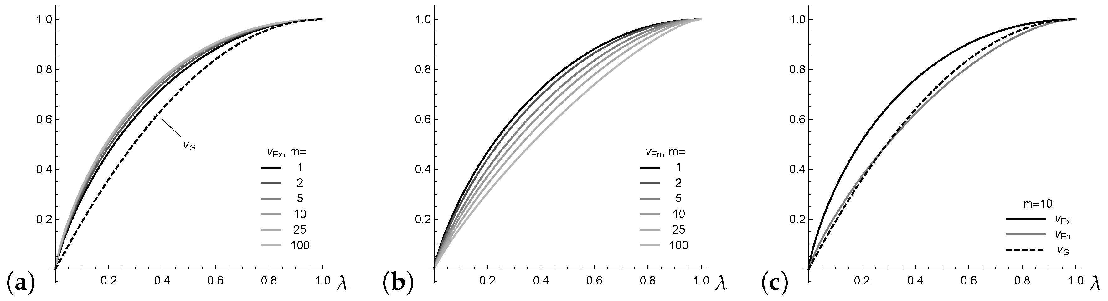
Things change, however, if considering the normalized versions ${\nu }_{\mathrm{Ex}}$, ${\nu }_{\mathrm{En}}$ and ${\nu }_{\mathrm{G}}$. For illustration, assume an underlying Lambda distribution $L_m\left(\lambda \right)$ with $\lambda \in (0;1)$ defined by the probability vector $p_{m;\lambda }={(1-\lambda +\frac{\lambda }{m+1},\frac{\lambda }{m+1},\dots ,\frac{\lambda }{m+1})}^{\top }$ (Kvålseth 2011a). Note that $\lambda \to 0$ leads to a one-point distribution, whereas $\lambda \to 1$ leads to the uniform distribution; actually, $L_m\left(\lambda \right)$ can be understood as a mixture of these boundary cases. For $L_m\left(\lambda \right)$, the Gini index satisfies ${\nu }_{\mathrm{G}}=\lambda (2-\lambda )$ for all $m\in \mathbb{N}$ (see Kvålseth (2011a)). In addition, the extropy ${\nu }_{\mathrm{Ex}}$ has rather stable values for varying m (see Figure 1a), whereas the entropy values in Figure 1b change greatly. This complicates the interpretation of the actual level of normalized entropy.

Figure 1. Normalized dispersion measures for Lambda distribution $L_m\left(\lambda \right)$ against $\lambda$: ${\nu }_{\mathrm{Ex}},{\nu }_{\mathrm{G}}$ in (a), ${\nu }_{\mathrm{En}}$ in (b), comparison for $m=10$ in (c).

Finally, the example $m=10$ plotted in Figure 1c shows that, in contrast to Equation (7), there is no fixed order between the normalized entropy ${\nu }_{\mathrm{En}}$ and Gini index ${\nu }_{\mathrm{G}}$. In this and many further numerical experiments, however, it could be observed that the inequalities ${\nu }_{\mathrm{Ex}}\ge {\nu }_{\mathrm{En}}$ and ${\nu }_{\mathrm{Ex}}\ge {\nu }_{\mathrm{G}}$ hold. These inequalities are formulated as a general conjecture here.

From now on, we turn towards the sample versions ${\widehat{\nu }}_{\mathrm{Ex}},{\widehat{\nu }}_{\mathrm{En}},{\widehat{\nu }}_{\mathrm{G}}$ of ${\nu }_{\mathrm{Ex}},{\nu }_{\mathrm{En}},{\nu }_{\mathrm{G}}$. These are obtained by replacing the probabilities $p_i,\mathit{p}$ by the respective estimates ${\widehat{p}}_i,\widehat{\mathit{p}}$, which are computed as relative frequencies from the given sample data $x_1,\dots ,x_n$. As detailed in Section 3, $x_1,\dots ,x_n$ are assumed as time series data, but we also consider the case of independent and identically distributed (i.i.d.) data.

3. Distribution of Sample Dispersion Measures

To be able to derive the asymptotic distribution of statistics computed from $X_1,\dots ,X_n$, Weiß (2013) assumed that the nominal process is $\varphi$-mixing with exponentially decreasing weights such that the CLT on p. 200 in Billingsley (1999) is applicable. This condition is not only satisfied in the i.i.d.-case, but also for, among others, the so-called NDARMA models as introduced by Jacobs and Lewis (1983) (see Appendix A.1 for details). Then, Weiß (2013) derived the asymptotic distribution of $\sqrt{n}\left(\widehat{\mathit{p}}-\mathit{p}\right)$, which is the normal distribution $N(\mathbf{0},\mathbf{\Sigma })$ with $\mathbf{\Sigma }={\left({\sigma }_{ij}\right)}_{i,j=0,\dots ,m}$ given by

$${\sigma }_{ij}=p_j({\delta }_{i,j}-p_i)+{\sum }_{h=1}^{\infty }\left(p_{ij}\left(h\right)+p_{ji}\left(h\right)-2p_i{p}_j\right).$$

(8)

Using this result, the asymptotic properties of ${\widehat{\nu }}_{\mathrm{G}}$, ${\widehat{\nu }}_{\mathrm{En}}$ and ${\widehat{\nu }}_{\mathrm{Ex}}$ can be derived, as shown in Appendix B.2. The following subsections present and compare these properties in detail.

3.1. Asymptotic Normality

As shown in Appendix B.2, provided that $\mathit{p}\ne {\mathit{p}}_{\mathrm{one}},{\mathit{p}}_{\mathrm{uni}}$, all variation measures ${\widehat{\nu }}_{\mathrm{G}}$, ${\widehat{\nu }}_{\mathrm{En}}$ and ${\widehat{\nu }}_{\mathrm{Ex}}$ are asymptotically normally distributed. More precisely, $\sqrt{n}({\widehat{\nu }}_{\mathrm{G}}-{\nu }_{\mathrm{G}})$ is asymptotically normally distributed with variance

$$\begin{array}{cc}\hfill {\sigma }_{\mathrm{G}}^2=& 4{\left(\frac{m+1}{m}\right)}^2\sum _{i,j=0}^m{p}_i{p}_j{\sigma }_{ij}\hfill \\ \hfill {\displaystyle \stackrel{\mathrm{Equation}\left(8\right)}{=}}& 4{\left(\frac{m+1}{m}\right)}^2\left(s_3\left(\mathit{p}\right)-s_2^2\left(\mathit{p}\right)\right)\left(1+2\sum _{h=1}^{\infty }\underset{=:\vartheta \left(h\right)}{\underbrace{\sum _{i,j=0}^m\frac{\left(p_{ij}\left(h\right)-p_i{p}_j\right)p_i{p}_j}{s_3\left(\mathit{p}\right)-s_2^2\left(\mathit{p}\right)}}}\right),\hfill \end{array}$$

(9)

a result already known from Weiß (2013). Here, $\vartheta \left(h\right)$ might be understood as a measure of serial dependence, in analogy to the measures in Equations (3), (4) and (6). In particular, $\vartheta \left(h\right)=0$ in the i.i.d.-case, and $\vartheta \left(h\right)=\kappa \left(h\right)$ for NDARMA processes (Appendix A.1).

Analogously, $\sqrt{n}({\widehat{\nu }}_{\mathrm{En}}-{\nu }_{\mathrm{En}})$ is asymptotically normally distributed with variance

$$\begin{array}{cc}\hfill {\sigma }_{\mathrm{En}}^2=& \sum _{i,j=0}^m\frac{1+ln{p}_i}{ln(m+1)}\frac{1+ln{p}_j}{ln(m+1)}{\sigma }_{ij}\hfill \\ \hfill \stackrel{\mathrm{Equation}\left(8\right)}{=}& \frac{1}{{\left(ln(m+1)\right)}^2}\left(\sum _{i=0}^m{p}_i{(ln{p}_i)}^2-{\left(\sum _{i=0}^m{p}_{i}ln{p}_i\right)}^2\right)\hfill \\ & {\displaystyle ·\left(1+2\sum _{h=1}^{\infty }\underset{=:{\vartheta }^{*}\left(h\right)}{\underbrace{\frac{{\sum }_{i,j=0}^m(1+ln{p}_i)(1+ln{p}_j)\left(p_{ij}\left(h\right)-p_i{p}_j\right)}{{\sum }_{i=0}^m{p}_i{(ln{p}_i)}^2-{\left({\sum }_{i=0}^m{p}_{i}ln{p}_i\right)}^2}}}\right).}\hfill \end{array}$$

(10)

In the i.i.d.-case, where the last factor becomes 1 (cf. Appendix A.1), this result was given by Blyth (1959), whereas the general expression in Equation (10) can be found in the work of Weiß (2013).

A novel result follows for the extropy, where $\sqrt{n}({\widehat{\nu }}_{\mathrm{Ex}}-{\nu }_{\mathrm{Ex}})$ is asymptotically normally distributed with variance

$$\begin{array}{cc}\hfill {\sigma }_{\mathrm{Ex}}^2=& \sum _{i,j=0}^m\frac{1+ln(1-p_i)}{mln\left(\frac{m+1}{m}\right)}\frac{1+ln(1-p_j)}{mln\left(\frac{m+1}{m}\right)}{\sigma }_{ij}\hfill \\ \hfill \stackrel{\mathrm{Equation}\left(8\right)}{=}& \frac{1}{{\left(mln\left(\frac{m+1}{m}\right)\right)}^2}\left(\sum _{i=0}^m{p}_i{\left(ln(1-p_i)\right)}^2-{\left(\sum _{i=0}^m{p}_{i}ln(1-p_i)\right)}^2\right)\hfill \\ & {\displaystyle ·\left(1+2\sum _{h=1}^{\infty }\underset{=:{\vartheta }^{\star }\left(h\right)}{\underbrace{\frac{{\sum }_{i,j=0}^m\left(1+ln(1-p_i)\right)\left(1+ln(1-p_j)\right)\left(p_{ij}\left(h\right)-p_i{p}_j\right)}{{\sum }_{i=0}^m{p}_i{\left(ln(1-p_i)\right)}^2-{\left({\sum }_{i=0}^m{p}_{i}ln(1-p_i)\right)}^2}}}\right).}\hfill \end{array}$$

(11)

Again, the last factor becomes 1 in the i.i.d.-case as ${\vartheta }^{\star }\left(h\right)=0$, and ${\vartheta }^{\star }\left(h\right)=\kappa \left(h\right)$ for NDARMA processes (Appendix A.1).

In Equations (9)–(11), the notations $\vartheta \left(h\right)$, ${\vartheta }^{*}\left(h\right)$ and ${\vartheta }^{\star }\left(h\right)$ have been introduced (see the respective expressions covered by the curly bracket) to highlight the similar structure of the asymptotic variances, and to locate the effect of serial dependence. Actually, one might use $\vartheta \left(h\right)$, ${\vartheta }^{*}\left(h\right)$ and ${\vartheta }^{\star }\left(h\right)$ as measures of serial dependence in categorical time series, although their definition is probably too complex for practical use. In Section 3.2, when analyzing the bias of ${\widehat{\nu }}_{\mathrm{G}}$, ${\widehat{\nu }}_{\mathrm{En}}$ and ${\widehat{\nu }}_{\mathrm{Ex}}$, analogous relations to the $\kappa$-measures defined in Section 1 are established.

3.2. Asymptotic Bias

In Appendix B.2, we express the variation measures ${\widehat{\nu }}_{\mathrm{G}}$, ${\widehat{\nu }}_{\mathrm{En}}$ and ${\widehat{\nu }}_{\mathrm{Ex}}$ as centered quadratic polynomials (at least approximately), and subsequently derive a bias formula. For the sample Gini index, it follows that

$$E\left[{\widehat{\nu }}_{\mathrm{G}}\right]\approx {\nu }_{\mathrm{G}}-\frac{1}{n}\frac{m+1}{m}{\sum }_{i=0}^m{\sigma }_{ii}\stackrel{\mathrm{Equation}\left(8\right)}{=}{\nu }_{\mathrm{G}}\left(1-\frac{1}{n}\left(1+2{\sum }_{h=1}^{\infty }\kappa \left(h\right)\right)\right).$$

(12)

This formula was also derived by Weiß (2013), and it leads to the exact corrective factor $(1-\frac{1}{n})$ in the i.i.d.-case. For ${\widehat{\nu }}_{\mathrm{En}},{\widehat{\nu }}_{\mathrm{Ex}}$, such bias formulae do not exist yet. However, from our derivations in Appendix B.2, we newly obtain that

$$\begin{array}{cc}\hfill E\left[{\widehat{\nu }}_{\mathrm{En}}\right]\approx & {\nu }_{\mathrm{En}}-\frac{1}{2n}\sum _{i=0}^m\frac{p_i^{-1}}{ln(m+1)}{\sigma }_{ii}\stackrel{\mathrm{Equation}\left(8\right)}{=}{\nu }_{\mathrm{En}}-\frac{1}{2n}\frac{m}{ln(m+1)}\left(1+2\sum _{h=1}^{\infty }{\kappa }^{*}\left(h\right)\right).\hfill \end{array}$$

(13)

In the i.i.d.-case, the last factor reduces to 1, and ${\kappa }^{*}\left(h\right)=\kappa \left(h\right)$ for NDARMA processes (Appendix A.1). Comparing Equations (12) and (13), we see that the effect of serial dependence on the bias is always expressed in terms of a $\kappa$-measure, using the ordinary $\kappa$ (Equation (3)) for the Gini index, and the modified $\kappa$ (Equation (4)) for the entropy. Concerning the extropy, it turns out that the newly proposed $\kappa$-measure from Equation (6) takes this role:

$$\begin{array}{cc}\hfill E\left[{\widehat{\nu }}_{\mathrm{Ex}}\right]\approx & {\nu }_{\mathrm{Ex}}-\frac{1}{2n}\sum _{i=0}^m\frac{{(1-p_i)}^{-1}}{mln\left(\frac{m+1}{m}\right)}{\sigma }_{ii}\stackrel{\mathrm{Equation}\left(8\right)}{=}{\nu }_{\mathrm{Ex}}-\frac{1}{2n}\frac{1}{mln\left(\frac{m+1}{m}\right)}\left(1+2\sum _{h=1}^{\infty }{\kappa }^{\star }\left(h\right)\right).\hfill \end{array}$$

(14)

In the i.i.d.-case, the last factor again reduces to 1, and also ${\kappa }^{\star }\left(h\right)=\kappa \left(h\right)$ holds for NDARMA processes (Appendix A.1). Altogether, Equations (12)–(14) show a unique structure regarding the effect of serial dependence. Furthermore, the computed bias corrections imply the relations ${\nu }_G\leftrightarrow \kappa$, ${\nu }_{\mathrm{En}}\leftrightarrow {\kappa }^{*}$ and ${\nu }_{\mathrm{Ex}}\leftrightarrow {\kappa }^{\star }$. The sample versions of $\kappa ,{\kappa }^{*},{\kappa }^{\star }$ are analyzed later in Section 5.

3.3. Asymptotic Properties for Uniform Distribution

The asymptotic normality established in Section 3.1 certainly does not apply to the deterministic case $\mathit{p}={\mathit{p}}_{\mathrm{one}}$, but we also have to exclude the boundary case of a uniform distribution ${\mathit{p}}_{\mathrm{uni}}$. As shown in Appendix B.2, the asymptotic distribution of ${\widehat{\nu }}_{\mathrm{G}}$, ${\widehat{\nu }}_{\mathrm{En}}$ and ${\widehat{\nu }}_{\mathrm{Ex}}$ in the uniform case is not a normal distribution but a quadratic-form one. All three statistics can be related to the Pearson’s ${\chi }^2$-statistic:

$$\left.\begin{array}{c}\hfill nm(1-{\widehat{\nu }}_{\mathrm{G}})=\\ \hfill 2nln(m+1)·(1-{\widehat{\nu }}_{\mathrm{En}})\approx \\ \hfill 2n{m}^{2}ln\left(\frac{m+1}{m}\right)·(1-{\widehat{\nu }}_{\mathrm{Ex}})\approx \end{array}\right\}n\sum _{j=0}^m\frac{{({\widehat{p}}_j-\frac{1}{m+1})}^2}{\frac{1}{m+1}}.$$

(15)

The actual asymptotic distribution can now be derived by applying Theorem 3.1 in Tan (1977) to the asymptotic result in Equation (8), which requires computing the eigenvalues of $\mathbf{\Sigma }$. In special cases, however, one is not faced with a general quadratic-form distribution but with a ${\chi }_m^2$-distribution; this happens for NDARMA processes and certainly in the i.i.d.-case (see Weiß (2013)). Then, defining $c=1+2{\sum }_{h=1}^{\infty }\kappa \left(h\right)$, it holds that Equation (15) asymptotically follows c times a ${\chi }_m^2$-distribution (with $c=1$ in the i.i.d.-case).

4. Simulations and Applications

Section 4.1 presents some simulation results regarding the quality of the asymptotic approximations for ${\widehat{\nu }}_{\mathrm{G}}$, ${\widehat{\nu }}_{\mathrm{En}}$ and ${\widehat{\nu }}_{\mathrm{Ex}}$ as derived in Section 3. Section 4.2 then applies these measures within a longitudinal study about the most important goals in politics in Germany.

4.1. Finite-Sample Performance of Dispersion Measures

In applications, the normal and ${\chi }^2$-distributions derived in Section 3 were used as an approximation to the true distribution of ${\widehat{\nu }}_{\mathrm{G}}$, ${\widehat{\nu }}_{\mathrm{En}}$ and ${\widehat{\nu }}_{\mathrm{Ex}}$. Therefore, the finite-sample performance of these approximations had to be analyzed, which was done by simulation (with 10,000 replications per scenario). In the tables provided by Appendix C, the simulated means (Table A1) and standard deviations (Table A2) for ${\widehat{\nu }}_{\mathrm{G}}$, ${\widehat{\nu }}_{\mathrm{En}}$ and ${\widehat{\nu }}_{\mathrm{Ex}}$ are reported and compared to the respective asymptotic approximations. Then, a common application scenario was considered, the computation of two-sided 95% confidence intervals (CIs) for ${\widehat{\nu }}_{\mathrm{G}}$, ${\widehat{\nu }}_{\mathrm{En}}$ and ${\widehat{\nu }}_{\mathrm{Ex}}$. Since the true parameter values are not known in practice, one has to plug-in estimated parameters into the formulae for mean and variance given in Section 3. The simulated coverage rates reported in Table A3 refer to such plug-in CIs. For these simulations, we either used an i.i.d. data-generating process (DGP) or an NDARMA DGP (see Appendix A.1): a DMA(1) process with ${\phi }_1=0.25$ or a DAR(1) process with ${\varphi }_1=0.40$. These were combined with the marginal distributions ($m=3$) summarized in Table 1: ${\mathit{p}}_1$ and ${\mathit{p}}_2$ were used before by Weiß (2011, 2013), ${\mathit{p}}_3$ by Kvålseth (2011b), and ${\mathit{p}}_4$ to ${\mathit{p}}_6$ are Lambda distributions $L_m\left(\lambda \right)$ with $\lambda \in \{0.25,0.50,0.75\}$ (see Kvålseth 2011a).

Table 1. Marginal distributions considered in Section 4.1 together with the corresponding dispersion values.

PMF	${\mathit{\nu }}_{\mathbf{G}}$	${\mathit{\nu }}_{\mathbf{En}}$	${\mathit{\nu }}_{\mathbf{Ex}}$
${\mathit{p}}_1={(0.2,0.2,0.25,0.35)}^{\top }$	0.980	0.979	0.988
${\mathit{p}}_2={(0.05,0.1,0.15,0.7)}^{\top }$	0.633	0.660	0.745
${\mathit{p}}_3={(0.2,0.15,0.05,0.6)}^{\top }$	0.767	0.767	0.848
${\mathit{p}}_4={(0.8125,0.0625,0.0625,0.0625)}^{\top }$	0.438	0.497	0.574
${\mathit{p}}_5={(0.625,0.125,0.125,0.125)}^{\top }$	0.750	0.774	0.832
${\mathit{p}}_6={(0.4375,0.1875,0.1875,0.1875)}^{\top }$	0.938	0.940	0.961

Finally, we used the results in Section 3.3 to test the null hypothesis (level 5%) of the uniform distribution $L_3\left(1\right)$ (${\nu }_{\mathrm{G}}={\nu }_{\mathrm{En}}={\nu }_{\mathrm{Ex}}=1$) based on ${\widehat{\nu }}_{\mathrm{G}}$, ${\widehat{\nu }}_{\mathrm{En}}$ and ${\widehat{\nu }}_{\mathrm{Ex}}$. The considered alternatives were $L_m\left(\lambda \right)$ with $\lambda \in \{0.98,0.96,0.94,0.92,0.90\}$, and the DGPs were as presented above. The simulated rejection rates are summarized in Table A4. Note that the required factor $c=1+2{\sum }_{h=1}^{\infty }\kappa \left(h\right)$ equald $c=(1+{\varphi }_1)/(1-{\varphi }_1)$ with ${\varphi }_1=\kappa \left(1\right)$ in the DAR(1) case, and $c=1+2\kappa \left(1\right)=1+2{\phi }_1(1-{\phi }_1)$ in the DMA(1) case, and was thus easy to estimate from the given time series data.

Let us now investigate the simulation results. Comparing the simulated mean values in Table A1 with the true dispersion values in Table 1, we realized a considerable negative bias for small sample sizes, which became even larger with increasing serial dependence. Fortunately, this bias is explained very well by the asymptotic bias correction, in any of the considered scenarios. With some limitations, this conclusion also applies to the standard deviations reported in Table A2; however, for sample size $n=100$ and increasing serial dependence, the discrepancy between asymptotic and simulated values increased. As a result, the coverage rates in Table A3 performed rather poorly for sample size 100; thus, reliable CIs generally required a sample of size at least 250. It should also be noted that Gini index and extropy performed very similarly and often slightly worse than the entropy. Finally, the rejection rates in Table A4 concerning the tests for uniformity showed similar sizes (columns “$1.00$”; slightly above 0.05 for $n=100$) but little different power values: best for extropy and worst for entropy.

4.2. Application: Goals in Politics

The monitoring of public mood and political attitudes over time is important for decision makers as well as for social scientists. Since 1980, the German General Social Survey (“ALLBUS”) is carried out by the “GESIS—Leibniz Institute for the Social Sciences” in every second year (exception: there was an additional survey in 1991 after the German reunification). In the years before and including 1990, the survey was done only in Western Germany, but in all Germany for the years 1991 and later. In what follows, we consider the cumulative report for 1980–2016 in GESIS—Leibniz Institute for the Social Sciences (2018), and there the question “If you had to choose between these different goals, which one would seem to you personally to be the most important?”. The four possible (nominal) answers are

• $s_0$: “To maintain law and order in this country”;
• $s_1$: “To give citizens more influence on government decisions”;
• $s_2$: “To fight rising prices”; and
• $s_3$: “To protect the right of freedom of speech”.

The sample sizes of this longitudinal study varied between 2795 and 3754, and are thus sufficiently large for the asymptotics derived in Section 3. If just looking at the mode as a summary measure (location), there is not much change in time: from 1980 to 2000 and again in 2016, the majority of respondents considered $s_0$ (law and order) as the most important goal in politics, whereas $s_1$ (influence) was judged most important between 2002 and 2014.

Much more fluctuations are visible if looking at the dispersion measures in Figure 2a. Although the absolute values of the measures differ, the general shapes of the graphs are quite similar. Usually, the dispersion measures take rather large values (≥0.90 in most of the years), which shows that any of the possible goals is considered as being most important by a large part of the population. On the other hand, the different goals never have the same popularity. Even in 2008, where all measures give a value very close to 1, the corresponding uniformity tests lead to a clear rejection of the null of a uniform distribution (p-values approximately 0 throughout).

Figure 2. ALLBUS data from Section 4.2: (a) dispersion measures; (b) extropy with 95% CIs; and (c) relative frequencies; plotted against year of survey.

Let us now analyze the development of the importance of the political goals in some more detail, by looking at the extropy for illustration. Figure 2b shows the approximate 95%-CIs in time (a bias correction does not have a visible effect because of the large sample sizes). There are phases where successive CIs overlap, and these are interrupted by breaks in the dispersion behavior. Such breaks happen, e.g., in 1984 (possibly related to a change of government in Germany in 1982/83), in 2002 (perhaps related to 9/11), or in 2008 and 2010 (Lehman bankruptcy and economic crisis). These changes in dispersion go along with reallocations of probability masses, as can be seen from Figure 2c. From the frequency curves of $s_0$ and $s_1$, we can see the above-mentioned change in mode, where the switch back to $s_0$ (law and order) might be caused by the refugee crisis. In addition, the curve for $s_2$ (fight rising prices) helps for explanation, as it shows that $s_2$ is important for the respondents in the beginning of the 1980s (where Germany suffered from very high inflation) and in 2008 (economic crisis), but not otherwise. Thus, altogether, the dispersion measures together with their approximate CIs give a very good summary of the distributional changes over time.

5. Measures of Signed Serial Dependence

After having discussed the analysis of marginal properties of a categorical time series, we now turn to the analysis of serial dependencies. In Section 1, two known measures of signed serial dependence, Cohen’s $\kappa \left(h\right)$ in Equation (3) and a modification of it, ${\kappa }^{*}\left(h\right)$ in Equation (4), are briefly surveyed, and, in Section 3.2, we realize a connection to ${\nu }_{\mathrm{G}}$ and ${\nu }_{\mathrm{En}}$, respectively. Motivated by a zero problem with ${\kappa }^{*}\left(h\right)$, a new type of modified $\kappa$ is proposed in Equation (6), the measure ${\kappa }^{\star }\left(h\right)$, and this turns out to be related to ${\nu }_{\mathrm{Ex}}$.

If replacing the (bivariate) probabilities in Equations (3), (4) and (6) by the respective (bivariate) relative frequencies computed from $x_1,\dots ,x_n$, we end up with sample versions of these dependence measures. Knowledge of their asymptotic distribution is particularly relevant for the i.i.d.-case, because this allows us to test for significant serial dependence in the given time series. As shown by Weiß (2011, 2013), $\widehat{\kappa }\left(h\right)$ then has an asymptotic normal distribution, and it holds approximately that

$$E\left[\widehat{\kappa }\left(h\right)\right]\approx -\frac{1}{n},V\left[\widehat{\kappa }\left(h\right)\right]\approx \frac{1}{n}\left(1-\frac{1+2s_3\left(\mathit{p}\right)-3s_2\left(\mathit{p}\right)}{{(1-s_2\left(\mathit{p}\right))}^2}\right).$$

(16)

The sample version of ${\kappa }^{*}\left(h\right)$ has a more simple asymptotic normal distribution with Weiß (2011, 2013)

$$E\left[{\widehat{\kappa }}^{*}\left(h\right)\right]\approx -\frac{1}{n},V\left[{\widehat{\kappa }}^{*}\left(h\right)\right]\approx \frac{1}{mn},$$

(17)

but it suffers from the before-mentioned zero problem, especially for short time series.

Thus, it remains to derive the asymptotics of the novel ${\widehat{\kappa }}^{\star }\left(h\right)$ under the null of an i.i.d. sample $X_1,\dots ,X_n$. The starting point is an extension of the limiting result in Equation (8). Under appropriate mixing assumptions (see Section 3), Weiß (2013) derived the joint asymptotic distribution of all univariate and equal-bivariate relative frequencies, i.e. of all $\sqrt{n}\left({\widehat{p}}_i-p_i\right)$ and $\sqrt{n}\left({\widehat{p}}_{jj}\left(h\right)-p_{jj}\left(h\right)\right)$, which is the $2(m+1)$-dimensional normal distribution $N(\mathbf{0},{\mathbf{\Sigma }}^{\left(h\right)})$. The covariance matrix ${\mathbf{\Sigma }}^{\left(h\right)}$ consists of four blocks with entries

$$\begin{array}{cc}\hfill {\sigma }_{i,j}=& p_j({\delta }_{i,j}-p_i)+\sum _{k=1}^{\infty }\left(p_{ij}\left(k\right)+p_{ji}\left(k\right)-2p_i{p}_j\right),\hfill \\ \hfill {\sigma }_{i,m+1+j}^{\left(h\right)}=& 2({\delta }_{i,j}-p_i)p_{jj}\left(h\right)+\sum _{k=1}^{\infty }\left(p_{ijj}(k,h)-p_i{p}_{jj}\left(h\right)\right)\hfill \\ & +\sum _{k=h+1}^{\infty }\left(p_{jji}(h,k-h)-p_i{p}_{jj}\left(h\right)\right)\hfill \\ & +\sum _{k=1}^{h-1}\left(p_{jij}(k,h-k)-p_i{p}_{jj}\left(h\right)\right)={\sigma }_{m+1+j,i}^{\left(h\right)},\hfill \\ \hfill {\sigma }_{m+1+i,m+1+j}^{\left(h\right)}=& \left({\delta }_{i,j}-p_{jj}\left(h\right)\right)p_{ii}\left(h\right)+2\left({\delta }_{i,j}{p}_{ijj}(h,h)-p_{ii}\left(h\right)p_{jj}\left(h\right)\right)\hfill \\ & +\sum _{k=1}^{h-1}\left(p_{jiji}(k,h-k,k)+p_{ijij}(k,h-k,k)-2p_{ii}\left(h\right)p_{jj}\left(h\right)\right)\hfill \\ & +\sum _{k=h+1}^{\infty }\left(p_{jjii}(h,k-h,h)+p_{iijj}(h,k-h,h)-2p_{ii}\left(h\right)p_{jj}\left(h\right)\right),\hfill \end{array}$$

(18)

where always $i,j=0,\dots ,m$, and where

$$\begin{array}{cc}\hfill p_{abc}(k,l)=& P(X_t=a,X_{t-k}=b,X_{t-k-l}=c),\hfill \\ \hfill p_{abcd}(k,l,m)=& P(X_t=a,X_{t-k}=b,X_{t-k-l}=c,X_{t-k-l-m}=d).\hfill \end{array}$$

This rather complex general result simplifies greatly special cases such as an NDARMA- DGP (Weiß 2013) and, in particular, for an i.i.d. DGP:

$$\begin{array}{cc}\hfill {\sigma }_{i,j}=& p_j({\delta }_{i,j}-p_i),\hfill \\ \hfill {\sigma }_{i,m+1+j}=& 2({\delta }_{i,j}-p_i)p_j^2={\sigma }_{m+1+j,i},\hfill \\ \hfill {\sigma }_{m+1+i,m+1+j}=& {\delta }_{i,j}{p}_i^2(1+2p_i)-3p_i^2{p}_j^2.\hfill \end{array}$$

(19)

Now, the asymptotic properties of ${\widehat{\kappa }}^{\star }\left(h\right)$ can be derived, as done in Appendix B.3. $\sqrt{n}\left({\widehat{\kappa }}^{\star }\left(h\right)-{\kappa }^{\star }\left(h\right)\right)$ is asymptotically normally distributed, and mean and variance can be approximated by plugging Equation (18) into

$$\begin{array}{cc}\hfill E\left[{\widehat{\kappa }}^{\star }\left(h\right)\right]\approx & {\displaystyle {\kappa }^{\star }\left(h\right)+\frac{1}{n}\sum _{j=0}^m\frac{(1-p_j){\sigma }_{j,m+1+j}^{\left(h\right)}-\left(1-p_{jj}\left(h\right)\right){\sigma }_{jj}}{{(1-p_j)}^3},}\hfill \\ \hfill V\left[{\widehat{\kappa }}^{\star }\left(h\right)\right]\approx & {\displaystyle \frac{1}{n}\sum _{i,j=0}^m\frac{p_{ii}\left(h\right)-2p_i+p_i^2}{{(1-p_i)}^2}\frac{p_{jj}\left(h\right)-2p_j+p_j^2}{{(1-p_j)}^2}{\sigma }_{i,j}}\hfill \\ & {\displaystyle +\sum _{i,j=0}^m\frac{{\sigma }_{m+1+i,m+1+j}^{\left(h\right)}}{(1-p_i)(1-p_j)}+2\sum _{i,j=0}^m\frac{p_{ii}\left(h\right)-2p_i+p_i^2}{{(1-p_i)}^2}\frac{{\sigma }_{i,m+1+j}^{\left(h\right)}}{1-p_j}.}\hfill \end{array}$$

(20)

In the i.i.d.-case, we simply have

$$E\left[{\widehat{\kappa }}^{\star }\left(h\right)\right]\approx -\frac{1}{n},V\left[{\widehat{\kappa }}^{\star }\left(h\right)\right]\approx \frac{1}{n}(s_2\left(p\right)-\sum _{i=0}^m{\left(\frac{p_i^2}{1-p_i}\right)}^2+{\left(\sum _{i=0}^m\frac{p_i^2}{1-p_i}\right)}^2).$$

(21)

Comparing Equations (16), (17) and (21), we see that all three measures have the same asymptotic bias $-1/n$, but their asymptotic variances generally differ. An exception to the latter statement is obtained in the case of a uniform distribution, then also the asymptotic variances coincide (see Appendix B.3).

6. Simulations and Applications

Section 6.1 presents some simulation results, where the quality of the asymptotic approximations for $\widehat{\kappa }\left(h\right),{\widehat{\kappa }}^{*}\left(h\right),{\widehat{\kappa }}^{\star }\left(h\right)$ according to Section 5 is investigated, as well as the power if testing against different types of serial dependence. Two real-data examples are discussed in Section 6.2 and Section 6.3, first an ordinal time series with rather strong positive dependence, then a nominal time series exhibiting negative dependencies.

6.1. Finite-Sample Performance of Serial Dependence Measures

In analogy to Section 4.1, we compared the finite-sample performance of the normal approximations in Equations (16), (17) and (21) via simulations1. As the power scenarios, we not only included NDARMA models but also the NegMarkov model described in Appendix A.2. These models were combined with the marginal distributions ${\mathit{p}}_1$ to ${\mathit{p}}_6$ in Table 1 plus ${\mathit{p}}_7={\mathit{p}}_{\mathrm{uni}}$; for the NegMarkov model, it was not possible to have the marginals ${\mathit{p}}_2$ and ${\mathit{p}}_4$ with very low dispersion. The full simulation results are available from the author upon request, but excerpts thereof are shown in the sequel to illustrate the main findings. As before, all tables are collected in Appendix C.

First, we discuss the distributional properties of $\widehat{\kappa }\left(h\right),{\widehat{\kappa }}^{*}\left(h\right),{\widehat{\kappa }}^{\star }\left(h\right)$ under the null of an i.i.d. DGP. The unique mean approximation $-1/n$ worked very well without exceptions. The quality of the standard deviations’ approximations is investigated in Table A5. Generally, the actual marginal dispersion was of great influence. For large dispersion (e.g., ${\mathit{p}}_6,{\mathit{p}}_7$ in Table A5), we had a very good agreement between asymptotic and simulated standard deviation, where deviations were typically not larger than $\pm 0.001$. For low dispersion (e.g., ${\mathit{p}}_5$ in Table A5), we found some discrepancy for $n=100$ and increasing h: the asymptotic approximation resulted in lower values for $\widehat{\kappa }\left(h\right),{\widehat{\kappa }}^{\star }\left(h\right)$ (discrepancy up to 0.004), and in larger values for ${\widehat{\kappa }}^{*}\left(h\right)$ (discrepancy up to 0.002). Consequently, if testing for serial independence, we expect the size for ${\widehat{\kappa }}^{*}\left(h\right)$ to be smaller than the nominal $5\%$-level, and to be larger for $\widehat{\kappa }\left(h\right),{\widehat{\kappa }}^{\star }\left(h\right)$. This was roughly confirmed by the results in Table A6 (and by further simulations), with the smallest size values for ${\widehat{\kappa }}^{*}\left(h\right)$ (might be smaller by up to 0.01) and the largest for ${\widehat{\kappa }}^{\star }\left(h\right)$. The sizes of $\widehat{\kappa }\left(h\right)$ tended to be smaller than 0.05 for $h=1$ (discrepancies $\le 0.003$), while those of ${\widehat{\kappa }}^{\star }\left(h\right)$ were always rather close to 5%.

A more complex picture was observed with regard to the power of $\widehat{\kappa }\left(h\right),{\widehat{\kappa }}^{*}\left(h\right),{\widehat{\kappa }}^{\star }\left(h\right)$ (see Table A6). For positive dependence (DMA(1) and DAR(1)), $\widehat{\kappa }\left(h\right),{\widehat{\kappa }}^{\star }\left(h\right)$ performed best if being close to a marginal uniform distribution, whereas ${\widehat{\kappa }}^{*}\left(h\right)$ had superior power for lower marginal dispersion levels (and $\widehat{\kappa }\left(h\right)$ performed second-best). For negative dependence (NegMarkov), in contrast, ${\widehat{\kappa }}^{\star }\left(h\right)$ was the optimal choice, and ${\widehat{\kappa }}^{*}\left(h\right)$ might have a rather poor power, especially for low dispersion. Thus, while $\widehat{\kappa }\left(h\right),{\widehat{\kappa }}^{\star }\left(h\right)$ both showed a more-or-less balanced performance with respect to positive and negative dependence, we had a sharp contrast for ${\widehat{\kappa }}^{*}\left(h\right)$.

6.2. Application: Fear Index

The Volatility Index (VIX) serves as a benchmark for U.S. stock market volatility, and increasing VIX values are interpreted as indications of greater fear in the market (Hancock 2012). Hancock (2012) distinguished between the $m+1=13$ ordinal fear states given in Table 2. From the historical closing rates of the VIX offered by the website https://finance.yahoo.com/, a time series of daily fear states was computed for the $n=4287$ trading days in the period 1990–2006 (before the beginning of the financial crisis). The obtained time series is plotted in Figure 3.

Table 2. Definition of fear states for Volatility Index (VIX) according to Hancock (2012).

State and Explanation		VIX	State and Explanation		VIX
$s_0$	extreme complacency	$[0;10)$	$s_7$	extremely high anx.	$[40;45)$
$s_1$	very low anx. = high compl.	$[10;15)$	$s_8$	near panic	$[45;50)$
$s_2$	low anx. = moderate compl.	$[15;20)$	$s_9$	moderate panic	$[50;55)$
$s_3$	moderate anx. = low compl.	$[20;25)$	$s_{10}$	panic	$[55;60)$
$s_4$	moderately high anxiety	$[25;30)$	$s_{11}$	intense panic	$[60;65)$
$s_5$	high anxiety	$[30;35)$	$s_{12}$	extreme panic	$[65;100]$
$s_6$	very high anxiety	$[35;40)$

Figure 3. Fear states time series plot and PMF (top); and plots of $\widehat{\kappa }\left(h\right),{\widehat{\kappa }}^{*}\left(h\right),{\widehat{\kappa }}^{\star }\left(h\right)$ (bottom).

As shown in the plots in the top panel of Figure 3, the states $s_9$–$s_{12}$ are never observed during 1990–2006, thus we have zero frequencies affecting the computation of ${\widehat{\nu }}_{\mathrm{En}}$ and ${\widehat{\kappa }}^{*}\left(h\right)$. The marginal distribution itself deviates visibly from a uniform distribution, thus it is reasonable that the dispersion measures ${\widehat{\nu }}_{\mathrm{G}}$, ${\widehat{\nu }}_{\mathrm{En}}$ and ${\widehat{\nu }}_{\mathrm{Ex}}$ are clearly below 1. Actually, the PMF mainly concentrates on the low to moderate fear states, high anxiety (or more) only happened for few of the trading days. Even more important is to investigate the development of these fear states over time. While negative serial dependence would indicate a permanent fluctuation between the states, positive dependence would imply some kind of inertia regarding the respective states. The serial dependence structure was analyzed, as shown in the bottom panel of Figure 3, where the critical values for level 5% (dashed lines) were computed according to the asymptotics in Section 5. All measures indicated significantly positive dependence, thus the U.S. stock market has a tendency to stay in a state once attained. However, ${\widehat{\kappa }}^{*}\left(h\right)$ (Figure 3, center) produced notably smaller values than $\widehat{\kappa }\left(h\right),{\widehat{\kappa }}^{\star }\left(h\right)$ (Figure 3, left and right). Considering that the time series plot with its long runs of single states implies a rather strong positive dependence, the values produced by ${\widehat{\kappa }}^{*}\left(h\right)$ did not appear to be that plausible. Thus, $\widehat{\kappa }\left(h\right),{\widehat{\kappa }}^{\star }\left(h\right)$, which resulted in very similar values, appeared to be better interpretable in the given example. Note that the discrepancy between ${\widehat{\kappa }}^{*}\left(h\right)$ and $\widehat{\kappa }\left(h\right),{\widehat{\kappa }}^{\star }\left(h\right)$ went along with the discrepancy between ${\widehat{\nu }}_{\mathrm{En}}$ and ${\widehat{\nu }}_{\mathrm{G}},{\widehat{\nu }}_{\mathrm{Ex}}$.

6.3. Application: Wood Pewee

Animal behavior studies are an integral part of research in biology and psychology. The time series example to be studied in the present section dates back to one of the pioneers of ethology, to Wallace Craig. The data were originally presented by Craig (1943) and further analyzed (among others) in Chapter 6 of the work by Weiß (2018). They constitute a nominal time series of length $n=1327$, where the three states $s_0,s_1,s_2$ express the different phrases in the morning twilight song of the Wood Pewee (“pee-ah-wee”, “pee-oh” and “ah-di-dee”, respectively). Since the range of a nominal time series lacks a natural order, a time series plot is not possible. Thus, Figure 4 shows a rate evolution graph as a substitute, where the cumulative frequencies of the individual states are plotted against time t. From the roughly linear increase, we conclude on a stable behavior of the time series (Weiß 2018).

Figure 4. Wood Pewee time series: rate evolution graph and PMF plot (top); and plots of $\widehat{\kappa }\left(h\right),{\widehat{\kappa }}^{*}\left(h\right),{\widehat{\kappa }}^{\star }\left(h\right)$ (bottom).

The dispersion measures ${\widehat{\nu }}_{\mathrm{G}}$, ${\widehat{\nu }}_{\mathrm{En}}$ and ${\widehat{\nu }}_{\mathrm{Ex}}$ all led to values between 0.90 and 0.95, indicating that all three phrases are frequently used (but not equally often) within the morning twilight song of the Wood Pewee. This is confirmed by the PMF plot in Figure 4, where we found some preference for the phrase $s_0$. From the serial dependence plots in the bottom panel of Figure 4, a quite complex serial dependence structure becomes visible, with both positive and negative dependence values and with a periodic pattern. Positive values happen for even lags h (and particularly large values for multiples of 4), and negative values for odd lags. The positive values indicate a tendency for repeating a phrase, and such repetitions seem to be particularly likely after every fourth phrase. Negative values, in contrast, indicate a change of the phrase, e.g., it will rarely happen that the same phrase is presented twice in a row. While $\widehat{\kappa }\left(h\right),{\widehat{\kappa }}^{\star }\left(h\right)$ gave a very clear (and similar) picture of the rhythmic structure, it was again ${\widehat{\kappa }}^{*}\left(h\right)$ that caused some implausible values, e.g., the non-significant value at lag 2. Thus, both data examples indicate that ${\widehat{\kappa }}^{*}\left(h\right)$ should be used with caution in practice (also because of the zero problem). A decision between $\widehat{\kappa }\left(h\right)$ and ${\widehat{\kappa }}^{\star }\left(h\right)$ is more difficult; $\widehat{\kappa }\left(h\right)$ is well established and slightly advantageous for uncovering positive dependencies, whereas ${\widehat{\kappa }}^{\star }\left(h\right)$ is computationally simpler and shows a very good performance regarding negative dependencies.

7. Conclusions

This work discusses approaches for measuring dispersion and serial dependence in categorical time series. Asymptotic properties of the novel extropy measure for categorical dispersion are derived and compared to those of Gini index and entropy. Simulations showed that all three measures performed quite well, with slightly better coverage rates for the entropy but computational advantages for Gini index and extropy. The extropy was most reliable if testing the null hypothesis of a uniform distribution. The application and interpretation of these measures was illustrated with a longitudinal study about the most important political goals in Germany.

The analysis of the asymptotic bias of Gini index, entropy and extropy uncovered a relation between these three measures and three types of $\kappa$-measures for signed serial dependence. While two of these measures, namely $\kappa \left(h\right)$ and ${\kappa }^{*}\left(h\right)$, have already been discussed in the literature, the “$\kappa$-counterpart” to the extropy turned out to be a new type of modified Cohen’s $\kappa$, denoted by ${\kappa }^{\star }\left(h\right)$. The asymptotics of ${\widehat{\kappa }}^{\star }\left(h\right)$ were investigated and utilized for testing for serial dependence. A simulation study as well as two real-data examples (time series of fear states and song of the Wood Pewee) showed that ${\widehat{\kappa }}^{*}\left(h\right)$ has several drawbacks, while both $\widehat{\kappa }\left(h\right)$ and ${\widehat{\kappa }}^{\star }\left(h\right)$ work very well in practice. The advantages of ${\widehat{\kappa }}^{\star }\left(h\right)$ are computational simplicity and a superior performance regarding negative dependencies.

Appendix A.1. NDARMA Models for Categorical Processes

The NDARMA model (“new” discrete autoregressive moving-average model) was proposed by Jacobs and Lewis (1983), and its definition might be given as follows (Weiß and Göb 2008):

Let ${\left(X_t\right)}_{\mathbb{Z}}$ and ${\left({ϵ}_t\right)}_{\mathbb{Z}}$ be categorical processes with state space $\mathcal{S}$, where ${\left({ϵ}_t\right)}_{\mathbb{Z}}$ is i.i.d. with marginal distribution p, and where ${ϵ}_t$ is independent of ${\left(X_s\right)}_{s<t}$. Let

$$({\alpha }_{t,1},\dots ,{\alpha }_{t,\mathrm{p}},{\beta }_{t,0},\dots ,{\beta }_{t,\mathrm{q}})\sim \mathrm{MULT}(1;{\varphi }_1,\dots ,{\varphi }_{\mathrm{p}},{\phi }_0,\dots ,{\phi }_{\mathrm{q}})$$

be i.i.d. multinomial random vectors, which are independent of ${\left({ϵ}_t\right)}_{\mathbb{Z}}$ and of ${\left(X_s\right)}_{s<t}$. Then, ${\left(X_t\right)}_{\mathbb{Z}}$ is said to be an NDARMA(p, q) process (and the cases $\mathrm{q}=0$ and $\mathrm{p}=0$ are referred to as a DAR(p) process and DMA(q) process, respectively) if it follows the recursion

$$X_t={\alpha }_{t,1}·X_{t-1}+\dots +{\alpha }_{t,\mathrm{p}}·X_{t-\mathrm{p}}+{\beta }_{t,0}·{ϵ}_t+\dots +{\beta }_{t,\mathrm{q}}·{ϵ}_{t-\mathrm{q}}.$$

(A1)

(Here, if the state space $\mathcal{S}$ is not numerically coded, we assume $0·s=0$, $1·s=s$ and $s+0=s$ for each $s\in \mathcal{S}$.)

NDARMA processes have several attractive properties, e.g. $X_t$ and ${ϵ}_t$ have the same stationary marginal distribution: $P(X_t=s_i)=p_i=P({ϵ}_t=s_i)$ for all $i\in \mathcal{S}$. Their serial dependence structure is characterized by a set of Yule–Walker-type equations for the serial dependence measure Cohen’s $\kappa$ from Equation (3) (Weiß and Göb 2008):

$$\kappa \left(h\right)={\sum }_{j=1}^{\mathrm{p}}{\varphi }_j\kappa \left(\right|h-j\left|\right)+{\sum }_{i=0}^{\mathrm{q}-h}{\phi }_{i+h}r\left(i\right)\mathrm{for}h\ge 1,$$

(A2)

where the $r\left(i\right)$ satisfy $r\left(i\right)={\sum }_{j=max\{0,i-\mathrm{p}\}}^{i-1}{\varphi }_{i-j}·r\left(j\right)+{\phi }_i\mathbb{1}(0\le i\le \mathrm{q})$. It should be noted that NDARMA processes satisfy $\kappa \left(h\right)\ge 0$, i.e. they can only handle positive serial dependence. Another important property is that the bivariate distributions at lag h are $p_{i|j}\left(h\right)=p_i+\kappa \left(h\right)({\delta }_{i,j}-p_i)$. This implies that $p_{ij}\left(h\right)-p_i{p}_j=\kappa \left(h\right)({\delta }_{i,j}-p_i)p_j$ and, as a consequence, that all of the serial dependence measures mentioned in this work coincide for NDARMA processes: $\vartheta \left(h\right)={\vartheta }^{*}\left(h\right)={\vartheta }^{\star }\left(h\right)=\kappa \left(h\right)={\kappa }^{*}\left(h\right)={\kappa }^{\star }\left(h\right)$.

Finally, Weiß (2013) showed that an NDARMA process is $\varphi$-mixing with exponentially decreasing weights such that the CLT on p. 200 in Billingsley (1999) is applicable.

Appendix A.2. Markov Chains for Categorical Processes

A discrete-valued Markov process ${\left(X_t\right)}_{\mathbb{Z}}$ is characterized by a “memory of length $\mathrm{p}\in \mathbb{N}$”, in the sense that

$$P(X_t=x_t|X_{t-1}=x_{t-1},\dots )=P(X_t=x_t|X_{t-1}=x_{t-1},\dots ,X_{t-\mathrm{p}}=x_{t-\mathrm{p}})$$

has to hold for all $x_i\in \mathcal{S}$. In the case $\mathrm{p}=1$, ${\left(X_t\right)}_{\mathbb{Z}}$ is commonly called a Markov chain. If the transition probabilities $P(X_t=i|X_{t-1}=j)$ of the Markov chain do not change with time t, i.e., if $P(X_t=i|X_{t-1}=j)=p_{i|j}$ for all $t\in \mathbb{N}$, it is said to be homogeneous (analogously for higher-order Markov processes). An example of a parsimoniously parametrized homogeneous Markov chain (Markov process) is the DAR(1) process (DAR(p) process) according to Appendix A.1, which always exhibits positive serial dependence.

A parsimoniously parametrized Markov model with negative serial dependence was proposed by Weiß (2011), the “Negative Markov model” (NegMarkov model). For a given probability vector $\mathit{\pi }\in {(0;1)}^{m+1}$ and some $\alpha \in (0;1]$, its transition probabilities are defined by

$$p_{i|j}=\left\{\begin{array}{cc}\alpha {\pi }_j\hfill & \mathrm{if}i=j,\hfill \\ {\beta }_j{\pi }_i\hfill & \mathrm{if}i\ne j,\hfill \end{array}\right.\mathrm{where}{\beta }_j=\frac{1-\alpha {\pi }_j}{1-{\pi }_j}\ge 1.$$

The resulting ergodic Markov chain has the stationary marginal distribution

$$p_j=\frac{{\pi }_j/{\beta }_j}{{\sum }_{i=0}^m{\pi }_i/{\beta }_i}\mathrm{for}j=0,\dots ,m.$$

As an example, if $\mathit{\pi }={\mathit{p}}_{\mathrm{uni}}$, then the ${\beta }_j$ become $1+(1-\alpha )/m$ such that p is also a uniform distribution. However, the conditional distribution given $X_{t-1}=j$ is not uniform:

$$p_{i|j}=\left\{\begin{array}{cc}\frac{\alpha }{m+1}\hfill & \mathrm{if}i=j,\hfill \\ (1+\frac{1-\alpha }{m})\frac{1}{m+1}\hfill & \mathrm{if}i\ne j.\hfill \end{array}\right.$$

Appendix B.1. Derivation of the inequality in Equation (7)

The first inequality in Equation (7) was shown by Lad et al. (2015). Using the inequality $ln(1+x)>x/(1+x/2)$ for $x>0$ from Love (1980), it follows for $p_i\in (0;1)$ that

$$-ln(1-p_i)=ln\left(1+\frac{p_i}{1-p_i}\right)>\frac{2p_i}{2-p_i},-ln{p}_i=ln\left(1+\frac{1-p_i}{p_i}\right)>2\frac{1-p_i}{1+p_i}.$$

Consequently, we have

$$-{\sum }_{i=0}^m(1-p_i)ln(1-p_i)\ge {\sum }_{i=0}^m{p}_i(1-p_i)\frac{2}{2-p_i}\ge 1-s_2\left(\mathit{p}\right),$$

as well as

$$-{\sum }_{i=0}^m{p}_{i}ln{p}_i\ge {\sum }_{i=0}^m{p}_i(1-p_i)\frac{2}{1+p_i}\ge 1-s_2\left(\mathit{p}\right).$$

Appendix B.2. Derivations for Sample Dispersion Measures

For studying the asymptotic properties of the sample Gini index according to Equation (1), it is important to know that ${\widehat{\nu }}_{\mathrm{G}}$ can be exactly rewritten as the centered quadratic polynomial

$${\widehat{\nu }}_{\mathrm{G}}={\nu }_G-2\frac{m+1}{m}{\sum }_{i=0}^m{p}_i({\widehat{p}}_i-p_i)-\frac{m+1}{m}{\sum }_{i=0}^m{({\widehat{p}}_i-p_i)}^2.$$

(A3)

Since $E\left[\widehat{\mathit{p}}\right]=\mathit{p}$ holds exactly, this representation immediately implies an exact way of bias computation, $n\left(E\left[{\widehat{\nu }}_{\mathrm{G}}\right]-{\nu }_{\mathrm{G}}\right)=\frac{m+1}{m}{\sum }_{i=0}^{m}V\left[\sqrt{n}({\widehat{p}}_i-p_i)\right]$, where $V\left[\sqrt{n}({\widehat{p}}_i-p_i)\right]$ is approximately given by ${\sigma }_{ii}$ according to Equation (8). Furthermore, provided that $\mathit{p}\ne {\mathit{p}}_{\mathrm{uni}}$, the resulting linear approximation together with the asymptotic normality of $\sqrt{n}\left(\widehat{\mathit{p}}-\mathit{p}\right)$ can be used to derive the asymptotic result (Equation (9)) (Delta method). Here, $\mathit{p}={\mathit{p}}_{\mathrm{uni}}$ has to be excluded, because then the linear term in Equation (A3) vanishes. Hence, in the boundary case $\mathit{p}={\mathit{p}}_{\mathrm{uni}}$, we end up with an asymptotic quadratic-form distribution instead of a normal one. Actually, it is easily seen that $nm(1-{\widehat{\nu }}_{\mathrm{G}})$ then coincides with the Pearson’s ${\chi }^2$-statistic with respect to ${\mathit{p}}_{\mathrm{uni}}$; see Section 4 in Weiß (2013) for the asymptotics.

For the entropy in Equation (2), an exact polynomial representation such as in Equation (A3) does not exist, thus we have to use a Taylor approximation instead:

$${\widehat{\nu }}_{\mathrm{En}}\approx {\nu }_{\mathrm{En}}-{\sum }_{j=0}^m\frac{1+ln{p}_j}{ln(m+1)}({\widehat{p}}_j-p_j)-\frac{1}{2}{\sum }_{j=0}^m\frac{p_j^{-1}}{ln(m+1)}{({\widehat{p}}_j-p_j)}^2.$$

(A4)

However, then, one can proceed as before. Thus, an approximate bias formula follows from

$$n\left(E\left[{\widehat{\nu }}_{\mathrm{En}}\right]-{\nu }_{\mathrm{En}}\right)\approx -\frac{1}{2}{\sum }_{j=0}^m\frac{p_j^{-1}}{ln(m+1)}V\left[\sqrt{n}({\widehat{p}}_j-p_j)\right]\approx -\frac{1}{2}{\sum }_{j=0}^m\frac{p_j^{-1}}{ln(m+1)}{\sigma }_{jj}.$$

For $\mathit{p}\ne {\mathit{p}}_{\mathrm{uni}}$, we can use the linear approximation implied by Equation (A4) to conclude on the asymptotic normality of $\sqrt{n}({\widehat{\nu }}_{\mathrm{En}}-{\nu }_{\mathrm{En}})$ with variance

$${\sigma }_{\mathrm{En}}^2=\sum _{i,j=0}^m\left(\frac{1+ln{p}_i}{ln(m+1)}\right)\left(\frac{1+ln{p}_j}{ln(m+1)}\right){\sigma }_{ij},$$

also see the results in (Blyth 1959; Weiß 2013). Note that, in the i.i.d.-case, where ${\sigma }_{ij}=p_j({\delta }_{i,j}-p_i)$, one computes

$$\begin{array}{c}\sum _{i,j=0}^m(1+ln{p}_i)(1+ln{p}_j)p_j({\delta }_{i,j}-p_i)\hfill \\ =\sum _{i=0}^m{(1+ln{p}_i)}^2{p}_i-{\left(\sum _{i=0}^m(1+ln{p}_i)p_i\right)}^2\hfill \\ =1+2\sum _{i=0}^m{p}_{i}ln{p}_i+\sum _{i=0}^m{p}_i{(ln{p}_i)}^2-{\left(1+\sum _{i=0}^m{p}_{i}ln{p}_i\right)}^2\hfill \\ =\sum _{i=0}^m{p}_i{(ln{p}_i)}^2-{\left(\sum _{i=0}^m{p}_{i}ln{p}_i\right)}^2.\hfill \end{array}$$

Finally, in the boundary case $\mathit{p}={\mathit{p}}_{\mathrm{uni}}$, again the linear term vanishes such that

$$2nln(m+1)·(1-{\widehat{\nu }}_{\mathrm{En}})\approx n\sum _{j=0}^m\frac{{({\widehat{p}}_j-\frac{1}{m+1})}^2}{\frac{1}{m+1}}$$

equals the Pearson’s ${\chi }^2$-statistic.

Finally, we do analogous derivations concerning the extropy in Equation (5). Starting with the Taylor approximation

$${\widehat{\nu }}_{\mathrm{Ex}}\approx {\nu }_{\mathrm{Ex}}+{\sum }_{j=0}^m\frac{1+ln(1-p_j)}{mln\left(\frac{m+1}{m}\right)}({\widehat{p}}_j-p_j)-\frac{1}{2}{\sum }_{j=0}^m\frac{{(1-p_j)}^{-1}}{mln\left(\frac{m+1}{m}\right)}{({\widehat{p}}_j-p_j)}^2,$$

(A5)

it follows that

$$n\left(E\left[{\widehat{\nu }}_{\mathrm{Ex}}\right]-{\nu }_{\mathrm{Ex}}\right)\approx -\frac{1}{2}{\sum }_{j=0}^m\frac{{(1-p_j)}^{-1}}{mln\left(\frac{m+1}{m}\right)}{\sigma }_{jj}.$$

For $\mathit{p}\ne {\mathit{p}}_{\mathrm{uni}}$, we can use the linear approximation implied by Equation (A5) to conclude on the asymptotic normality of $\sqrt{n}({\widehat{\nu }}_{\mathrm{Ex}}-{\nu }_{\mathrm{Ex}})$ with variance

$${\sigma }_{\mathrm{Ex}}^2=\sum _{i,j=0}^m\frac{1+ln(1-p_i)}{mln\left(\frac{m+1}{m}\right)}\frac{1+ln(1-p_j)}{mln\left(\frac{m+1}{m}\right)}{\sigma }_{ij}.$$

Note that, in the i.i.d.-case, where ${\sigma }_{ij}=p_j({\delta }_{i,j}-p_i)$, one computes

$$\begin{array}{c}\sum _{i,j=0}^m\left(1+ln(1-p_i)\right)\left(1+ln(1-p_j)\right)p_j({\delta }_{i,j}-p_i)\hfill \\ =\sum _{i=0}^m{p}_i{\left(ln(1-p_i)\right)}^2-{\left(\sum _{i=0}^m{p}_{i}ln(1-p_i)\right)}^2\hfill \end{array}$$

as before. Finally, in the boundary case $\mathit{p}={\mathit{p}}_{\mathrm{uni}}$, again the linear term vanishes such that

$$2n{m}^{2}ln\left(\frac{m+1}{m}\right)·(1-{\widehat{\nu }}_{\mathrm{Ex}})\approx n\sum _{j=0}^m\frac{{({\widehat{p}}_j-\frac{1}{m+1})}^2}{\frac{1}{m+1}}$$

equals the Pearson’s ${\chi }^2$-statistic.

Appendix B.3. Derivations for Measures of Signed Serial Dependence

We partition $x\in {(0;1)}^{2(m+1)}$ as $x={(x_0,\dots ,x_m,x_{m+1+0},\dots ,x_{m+1+m})}^{\top }$, and we define

$$f\left(x\right)=\sum _{j=0}^m\frac{x_{m+1+j}-x_j^2}{1-x_j}.$$

Then,

$$\frac{\partial }{\partial x_j}f\left(x\right)=\frac{x_{m+1+j}-2x_j+x_j^2}{{(1-x_j)}^2},\frac{\partial }{\partial x_{m+1+j}}f\left(x\right)=\frac{1}{1-x_j},$$

and

$$\frac{{\partial }^2}{\partial x_j{}^2}f\left(x\right)=\frac{-2(1-x_{m+1+j})}{{(1-x_j)}^3},\frac{{\partial }^2}{\partial x_j\partial x_{m+1+j}}f\left(x\right)=\frac{1}{{(1-x_j)}^2},$$

all other second-order derivatives equal 0. Thus, a second-order Taylor approximation of ${\widehat{\kappa }}^{\star }\left(h\right)=f\left(\dots ,{\widehat{p}}_j,\dots ,{\widehat{p}}_{jj}\left(h\right),\dots \right)$ is given by

$$\begin{array}{ccc}\hfill {\widehat{\kappa }}^{\star }\left(h\right)& \approx & {\kappa }^{\star }\left(h\right)+\sum _{j=0}^m\frac{p_{jj}\left(h\right)-2p_j+p_j^2}{{(1-p_j)}^2}\left({\widehat{p}}_j-p_j\right)+\sum _{j=0}^m\frac{1}{1-p_j}\left({\widehat{p}}_{jj}\left(h\right)-p_{jj}\left(h\right)\right)\hfill \\ & & -\sum _{j=0}^m\frac{1-p_{jj}\left(h\right)}{{(1-p_j)}^3}{\left({\widehat{p}}_j-p_j\right)}^2+\sum _{j=0}^m\frac{1}{{(1-p_j)}^2}\left({\widehat{p}}_j-p_j\right)\left({\widehat{p}}_{jj}\left(h\right)-p_{jj}\left(h\right)\right).\hfill \end{array}$$

Hence, using Equation (18), it follows that

$$\begin{array}{ccc}\hfill n\left(E\left[{\widehat{\kappa }}^{\star }\left(h\right)\right]-{\kappa }^{\star }\left(h\right)\right)& \approx & \sum _{j=0}^m\frac{1}{{(1-p_j)}^2}{\sigma }_{j,m+1+j}^{\left(h\right)}-\sum _{j=0}^m\frac{1-p_{jj}\left(h\right)}{{(1-p_j)}^3}{\sigma }_{jj}\hfill \\ & =& \sum _{j=0}^m\frac{(1-p_j){\sigma }_{j,m+1+j}^{\left(h\right)}-\left(1-p_{jj}\left(h\right)\right){\sigma }_{jj}}{{(1-p_j)}^3}.\hfill \end{array}$$

Furthermore, the Delta method implies that $\sqrt{n}\left({\widehat{\kappa }}^{\star }\left(h\right)-{\kappa }^{\star }\left(h\right)\right)\sim N(0,{\sigma }^2)$ with

$$\begin{array}{ccc}\hfill {\sigma }^2& =& \sum _{i,j=0}^m\frac{p_{ii}\left(h\right)-2p_i+p_i^2}{{(1-p_i)}^2}\frac{p_{jj}\left(h\right)-2p_j+p_j^2}{{(1-p_j)}^2}{\sigma }_{i,j}\hfill \\ & & +\sum _{i,j=0}^m\frac{{\sigma }_{m+1+i,m+1+j}^{\left(h\right)}}{(1-p_i)(1-p_j)}+2\sum _{i,j=0}^m\frac{p_{ii}\left(h\right)-2p_i+p_i^2}{{(1-p_i)}^2}\frac{{\sigma }_{i,m+1+j}^{\left(h\right)}}{1-p_j}.\hfill \end{array}$$

Note that, under the null of an i.i.d. DGP, we have the simplifications

$$\frac{p_{jj}\left(h\right)-2p_j+p_j^2}{{(1-p_j)}^2}=\frac{-2p_j}{1-p_j},\frac{1-p_{jj}\left(h\right)}{{(1-p_j)}^3}=\frac{1+p_j}{{(1-p_j)}^2}.$$

Thus, the second-order Taylor approximation of ${\widehat{\kappa }}^{\star }\left(h\right)$ then simplifies to

$$\begin{array}{ccc}\hfill {\widehat{\kappa }}^{\star }\left(h\right)& \approx & {\kappa }^{\star }\left(h\right)+\sum _{j=0}^m\frac{-2p_j}{1-p_j}\left({\widehat{p}}_j-p_j\right)+\sum _{j=0}^m\frac{1}{1-p_j}\left({\widehat{p}}_{jj}\left(h\right)-p_j^2\right)\hfill \\ & & -\sum _{j=0}^m\frac{1+p_j}{{(1-p_j)}^2}{\left({\widehat{p}}_j-p_j\right)}^2+\sum _{j=0}^m\frac{1}{{(1-p_j)}^2}\left({\widehat{p}}_j-p_j\right)\left({\widehat{p}}_{jj}\left(h\right)-p_j^2\right).\hfill \end{array}$$

Furthermore,

$${\sigma }_{i,j}=p_j({\delta }_{i,j}-p_i),{\sigma }_{i,m+1+j}=2p_j^2({\delta }_{i,j}-p_i),{\sigma }_{m+1+i,m+1+j}={\delta }_{i,j}{p}_i^2(1+2p_i)-3p_i^2{p}_j^2,$$

according to Equation (19). Thus, for an i.i.d. DGP, it follows that

$$\begin{array}{ccc}\hfill n\left(E\left[{\widehat{\kappa }}^{\star }\left(h\right)\right]-{\kappa }^{\star }\left(h\right)\right)=nE\left[{\widehat{\kappa }}^{\star }\left(h\right)\right]& \approx & \sum _{j=0}^m\frac{{\sigma }_{j,m+1+j}-(1+p_j){\sigma }_{jj}}{{(1-p_j)}^2}\hfill \\ & =& \sum _{j=0}^m\frac{2p_j^2(1-p_j)-(1+p_j)p_j(1-p_j)}{{(1-p_j)}^2}\hfill \\ & =& \sum _{j=0}^m\frac{-p_j(1-p_j)(1+p_j-2p_j)}{{(1-p_j)}^2}=-1.\hfill \end{array}$$

Furthermore,

$$\begin{array}{ccc}\hfill {\sigma }^2& =& \sum _{i,j=0}^m\frac{-2p_i}{1-p_i}\frac{-2p_j}{1-p_j}{p}_j({\delta }_{i,j}-p_i)+2\sum _{i,j=0}^m\frac{-2p_i}{1-p_i}\frac{1}{1-p_j}2p_j^2({\delta }_{i,j}-p_i)\hfill \\ & & +\sum _{i,j=0}^m\frac{1}{1-p_i}\frac{1}{1-p_j}\left({\delta }_{i,j}{p}_i^2(1+2p_i)-3p_i^2{p}_j^2\right)\hfill \\ & =& 4\sum _{i=0}^m\frac{p_i^3}{{(1-p_i)}^2}-8\sum _{i=0}^m\frac{p_i^3}{{(1-p_i)}^2}+\sum _{i=0}^m\frac{p_i^2(1+2p_i)}{{(1-p_i)}^2}\hfill \\ & & -4\sum _{i,j=0}^m\frac{p_i^2}{1-p_i}\frac{p_j^2}{1-p_j}+8\sum _{i,j=0}^m\frac{p_i^2}{1-p_i}\frac{p_j^2}{1-p_j}-3\sum _{i,j=0}^m\frac{p_i^2}{1-p_i}\frac{p_j^2}{1-p_j}\hfill \\ & =& \sum _{i=0}^m\frac{p_i^2(1-2p_i)}{{(1-p_i)}^2}+(\sum _{i=0}^m\frac{p_i^2}{1-p_i}{)}^2.\hfill \end{array}$$

This leads to Equation (21).

In the special case of a uniform distribution, i.e. where all $p_i=\frac{1}{m+1}$, the asymptotic variances according to Equations (16), (17) and (21) coincide. Then, we have in Equation (16) that

$$1-\frac{1+2s_3\left(\mathit{p}\right)-3s_2\left(\mathit{p}\right)}{{(1-s_2\left(\mathit{p}\right))}^2}=1-\frac{1+\frac{2}{{(m+1)}^2}-\frac{3}{m+1}}{{(1-\frac{1}{m+1})}^2}=1-\frac{{(m+1)}^2+2-3(m+1)}{m^2}=1-\frac{m^2-m}{m^2}=\frac{1}{m},$$

which corresponds to Equation (17). However, the same expression also follows in Equation (21):

$$s_2\left(\mathit{p}\right)-{\sum }_{i=0}^m{\left(\frac{p_i^2}{1-p_i}\right)}^2+{\left({\sum }_{i=0}^m\frac{p_i^2}{1-p_i}\right)}^2=\frac{1}{m+1}-\frac{1}{m^2(m+1)}+\frac{1}{m^2}=\frac{1}{m}.$$

References

1. Agresti, Alan. 2002. Categorical Data Analysis, 2nd ed.Hoboken: John Wiley & Sons, Inc. [Google Scholar]
2. Billingsley, Patrick. 1999. Convergence of Probability Measures, 2nd ed.New York: John Wiley & Sons, Inc. [Google Scholar]
3. Blyth, Colin R. 1959. Note on estimating information. Annals of Mathematical Statistics 30: 71–79. [Google Scholar] [CrossRef]
4. Cohen, Jacob. 1960. A coefficient of agreement for nominal scales. Educational and Psychological Measurement 20: 37–46. [Google Scholar] [CrossRef]
5. Craig, Wallace. 1943. The Song of the Wood Pewee, Myiochanes virens Linnaeus: A Study of Bird Music. New York State Museum Bulletin No. 334. Albany: University of the State of New York. [Google Scholar]
6. GESIS—Leibniz Institute for the Social Sciences. 2018. ALLBUS 1980–2016 (German General Social Survey). ZA4586 Data File (Version 1.0.0). Cologne: GESIS Data Archive. (In German) [Google Scholar]
7. Hancock, Gwendolyn D’Anne. 2012. VIX and VIX futures pricing algorithms: Cultivating understanding. Modern Economy 3: 284–94. [Google Scholar]
8. Jacobs, Patricia A., and Peter A. W. Lewis. 1983. Stationary discrete autoregressive-moving average time series generated by mixtures. Journal of Time Series Analysis 4: 19–36. [Google Scholar] [CrossRef]
9. Kvålseth, Tarald O. 1995. Coefficients of variation for nominal and ordinal categorical data. Perceptual and Motor Skills 80: 843–47. [Google Scholar] [CrossRef]
10. Kvålseth, Tarald O. 2011a. The lambda distribution and its applications to categorical summary measures. Advances and Applications in Statistics 24: 83–106. [Google Scholar]
11. Kvålseth, Tarald O. 2011b. Variation for categorical variables. In International Encyclopedia of Statistical Science. Edited by Miodrag Lovric. Berlin: Springer, pp. 1642–45. [Google Scholar]
12. Lad, Frank, Giuseppe Sanfilippo, and Gianna Agro. 2015. Extropy: Complementary dual of entropy. Statistical Science 30: 40–58. [Google Scholar] [CrossRef]
13. Love, Eric Russell. 1980. Some logarithm inequalities. Mathematical Gazette 64: 55–57. [Google Scholar] [CrossRef]
14. Rao, C. Radhakrishna. 1982. Diversity and dissimilarity coefficients: A unified approach. Theoretical Population Biology 21: 24–43. [Google Scholar] [CrossRef]
15. Shannon, Claude Elwood. 1948. A mathematical theory of communication. Bell System Technical Journal 27: 379–423, 623–56. [Google Scholar] [CrossRef]
16. Shorrocks, Anthony F. 1978. The measurement of mobility. Econometrica 46: 1013–24. [Google Scholar] [CrossRef]
17. Tan, Wai-Yuan. 1977. On the distribution of quadratic forms in normal random variables. Canadian Journal of Statististics 5: 241–50. [Google Scholar] [CrossRef]
18. Weiß, Christian H. 2011. Empirical measures of signed serial dependence in categorical time series. Journal of Statistical Computation and Simulation 81: 411–29. [Google Scholar] [CrossRef]
19. Weiß, Christian H. 2013. Serial dependence of NDARMA processes. Computational Statistics and Data Analysis 68: 213–38. [Google Scholar] [CrossRef]
20. Weiß, Christian H. 2018. An Introduction to Discrete-Valued Time Series. Chichester: John Wiley & Sons, Inc. [Google Scholar]
21. Weiß, Christian H., and Rainer Göb. 2008. Measuring serial dependence in categorical time series. AStA Advances in Statistical Analysis 92: 71–89. [Google Scholar] [CrossRef]
1.
The “zero problem” for κ * ( h ) described after Equation (4) happened mainly for n = 100 and for distributions with low dispersion such as p 2 to p 4 , in about 0.5% of the i.i.d. simulation runs. It increased with positive dependence, to about 2% for the DAR(1) simulation runs. This problem was circumvented by replacing all affected summands by 0.