An Overview of Modified Semiparametric Memory Estimation Methods

Abstract
1. Introduction
2. Semiparametric Estimation Methods
2.1. The Model and Standard Estimation Methods
2.2. Modified Log-Periodogram Estimator of Smith (2005)
2.3. Modified Local Whittle Estimator of Iacone (2010)
2.4. Modified Log-Periodogram Estimator of McCloskey and Perron (2013)
2.5. Modified Local Whittle Estimator of Hou and Perron (2014)
2.6. Local Polynomial Whittle Estimator of Andrews and Sun (2004)
2.7. Local Whittle with Noise Estimator of Hurvich et al. (2005)
2.8. Local Polynomial Whittle with Noise Estimator of Frederiksen et al. (2012)
3. Monte Carlo Analysis
3.1. Monte Carlo Setup
3.2. Monte Carlo Results
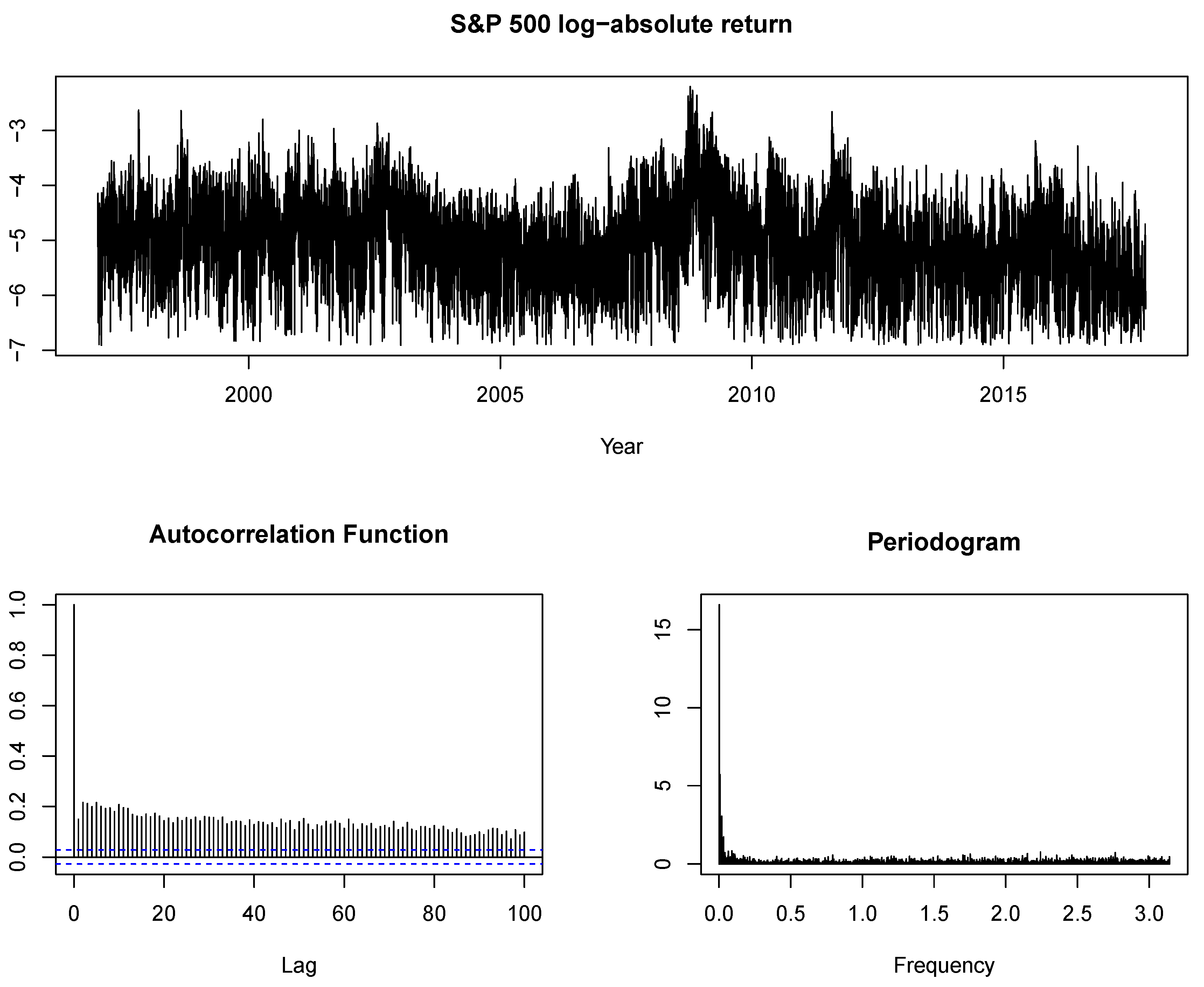
4. Application
5. Conclusions
Supplementary Materials
Author Contributions
Conflicts of Interest
References
- Andrews, Donald W.K., and Yixiao Sun. 2004. Adaptive local polynomial Whittle estimation of long-range dependence. Econometrica 72: 569–614. [Google Scholar] [CrossRef]
- Arteche, Josu. 2004. Gaussian semiparametric estimation in long memory in stochastic volatility and signal plus noise models. Journal of Econometrics 119: 131–54. [Google Scholar] [CrossRef]
- Arteche, Josu. 2006. Semiparametric estimation in perturbed long memory series. Computational Statistics & Data Analysis 51: 2118–141. [Google Scholar]
- Byrd, Richard H., Peihuang Lu, Jorge Nocedal, and Ciyou Zhu. 1995. A limited memory algorithm for bound constrained optimization. SIAM Journal on Scientific Computing 16: 1190–208. [Google Scholar] [CrossRef]
- Diebold, Francis X., and Atsushi Inoue. 2001. Long memory and regime switching. Journal of Econometrics 105: 131–59. [Google Scholar] [CrossRef]
- Doukhan, Paul, George Oppenheim, and Murad Taqqu. 2002. Theory and Applications of Long-Range Dependence. Berlin: Springer Science & Business Media. [Google Scholar]
- Faÿ, Gilles, Eric Moulines, François Roueff, and Murad S. Taqqu. 2009. Estimators of long-memory: Fourier versus wavelets. Journal of Econometrics 151: 159–77. [Google Scholar] [CrossRef]
- Frederiksen, Per, Frank S. Nielsen, and Morten Ørregaard Nielsen. 2012. Local polynomial Whittle estimation of perturbed fractional processes. Journal of Econometrics 167: 426–47. [Google Scholar] [CrossRef]
- Frederiksen, Per, and Morten Ørregaard Nielsen. 2008. Bias-reduced estimation of long-memory stochastic volatility. Journal of Financial Econometrics 6: 496–512. [Google Scholar] [CrossRef]
- Geweke, John, and Susan Porter-Hudak. 1983. The estimation and application of long memory time series models. Journal of Time Series Analysis 4: 221–38. [Google Scholar] [CrossRef]
- Granger, Clive W. J., and Namwon Hyung. 2004. Occasional structural breaks and long memory with an application to the S&P 500 absolute stock returns. Journal of Empirical Finance 11: 399–421. [Google Scholar]
- Granger, Clive W. J., and Roselyne Joyeux. 1980. An introduction to long-memory time series models and fractional differencing. Journal of Time Series Analysis 1: 15–29. [Google Scholar] [CrossRef]
- Haldrup, Niels, and Morten Ørregaard Nielsen. 2007. Estimation of fractional integration in the presence of data noise. Computational Statistics & Data Analysis 51: 3100–14. [Google Scholar]
- Hosking, Jonathan R. M. 1981. Fractional differencing. Biometrika 68: 165–76. [Google Scholar] [CrossRef]
- Hou, Jie, and Pierre Perron. 2014. Modified local Whittle estimator for long memory processes in the presence of low frequency (and other) contaminations. Journal of Econometrics 182: 309–28. [Google Scholar] [CrossRef]
- Hurvich, Clifford M., Eric Moulines, and Philippe Soulier. 2005. Estimating long memory in volatility. Econometrica 73: 1283–328. [Google Scholar] [CrossRef]
- Hurvich, Clifford M., and Bonnie K. Ray. 2003. The local Whittle estimator of long-memory stochastic volatility. Journal of Financial Econometrics 1: 445–70. [Google Scholar] [CrossRef]
- Iacone, Fabrizio. 2010. Local Whittle estimation of the memory parameter in presence of deterministic components. Journal of Time Series Analysis 31: 37–49. [Google Scholar] [CrossRef]
- Kuensch, Hans R. 1987. Statistical aspects of self-similar processes. Paper presented at First World Congress of the Bernoulli Society, Tashkent, Uzbekistan, September 8–14; pp. 67–74. [Google Scholar]
- Lu, Yang K., and Pierre Perron. 2010. Modeling and forecasting stock return volatility using a random level shift model. Journal of Empirical Finance 17: 138–56. [Google Scholar] [CrossRef]
- McCloskey, Adam. 2013. Estimation of the long-memory stochastic volatility model parameters that is robust to level shifts and deterministic trends. Journal of Time Series Analysis 34: 285–301. [Google Scholar] [CrossRef]
- McCloskey, Adam, and Jonathan B. Hill. 2017. Parameter estimation robust to low-frequency contamination. Journal of Business & Economic Statistics 35: 598–610. [Google Scholar]
- McCloskey, Adam, and Pierre Perron. 2013. Memory parameter estimation in the presence of level shifts and deterministic trends. Econometric Theory 29: 1196–237. [Google Scholar] [CrossRef]
- Perron, Pierre, and Zhongjun Qu. 2010. Long-memory and level shifts in the volatility of stock market return indices. Journal of Business & Economic Statistics 28: 275–90. [Google Scholar]
- Qu, Zhongjun. 2011. A test against spurious long memory. Journal of Business & Economic Statistics 29: 423–38. [Google Scholar]
- Qu, Zhongjun, and Pierre Perron. 2013. A stochastic volatility model with random level shifts and its applications to S&P 500 and NASDAQ return indices. The Econometrics Journal 16: 309–39. [Google Scholar]
- Robinson, Peter M. 1995. Log-periodogram regression of time series with long range dependence. The Annals of Statistics 23: 1048–72. [Google Scholar] [CrossRef]
- Smith, Aaron. 2005. Level shifts and the illusion of long memory in economic time series. Journal of Business & Economic Statistics 23: 321–35. [Google Scholar]
- Sun, Yixiao, and Peter C. B. Phillips. 2003. Nonlinear log-periodogram regression for perturbed fractional processes. Journal of Econometrics 115: 355–89. [Google Scholar] [CrossRef]
- Wenger, Kai, Christian Leschinski, and Philipp Sibbertsen. 2017. The Memory of Volatility. Unpublished Manuscript. Hanover, Germany: Department of Economics, University of Hannover. [Google Scholar]
- Xu, Jiawen, and Pierre Perron. 2014. Forecasting return volatility: Level shifts with varying jump probability and mean reversion. International Journal of Forecasting 30: 449–63. [Google Scholar] [CrossRef]
- Yamamoto, Yohei, and Pierre Perron. 2013. Estimating and testing multiple structural changes in linear models using band spectral regressions. The Econometrics Journal 16: 400–29. [Google Scholar] [CrossRef][Green Version]


| no contamination | ||
| sinus trend | ||
| stationary RLS | ||
| Bernoulli | ||
| non-stationary RLS | ||
| Bernoulli | ||
| deterministic level shift | ||
| GARCH (1,1) | ||
| ARMA(0,0) | ||
| ARMA(0,1) | ||
| stationary RLS plus noise | ||
| Bernoulli | ||
| d | 0.0 | 0.2 | 0.4 | 0.0 | 0.2 | 0.4 | 0.0 | 0.2 | 0.4 | |||||||||
|---|---|---|---|---|---|---|---|---|---|---|---|---|---|---|---|---|---|---|
| 0.70 | 0.79 | 0.70 | 0.79 | 0.70 | 0.79 | 0.70 | 0.79 | 0.70 | 0.79 | 0.70 | 0.79 | 0.70 | 0.79 | 0.70 | 0.79 | 0.70 | 0.79 | |
| Bias | ||||||||||||||||||
| 0.661 | 0.524 | 0.457 | 0.350 | 0.297 | 0.215 | 0.614 | 0.527 | 0.432 | 0.375 | 0.300 | 0.268 | 0.614 | 0.596 | 0.470 | 0.485 | 0.374 | 0.420 | |
| 0.119 | 0.075 | 0.095 | 0.063 | 0.080 | 0.047 | 0.153 | 0.171 | 0.131 | 0.158 | 0.114 | 0.148 | 0.267 | 0.369 | 0.246 | 0.355 | 0.234 | 0.349 | |
| −0.311 | −0.147 | −0.288 | −0.145 | −0.275 | −0.160 | −0.158 | 0.059 | −0.154 | 0.048 | −0.159 | 0.037 | 0.121 | 0.371 | 0.119 | 0.374 | 0.161 | 0.413 | |
| 0.002 | 0.002 | −0.007 | −0.008 | −0.007 | −0.017 | 0.070 | 0.185 | 0.057 | 0.173 | 0.063 | 0.167 | 0.293 | 0.519 | 0.288 | 0.513 | 0.293 | 0.503 | |
| −0.082 | −0.015 | −0.041 | −0.007 | 0.020 | 0.006 | 0.060 | 0.159 | 0.045 | 0.131 | 0.096 | 0.148 | 0.252 | 0.371 | 0.250 | 0.362 | 0.335 | 0.503 | |
| 0.287 | 0.179 | 0.234 | 0.146 | 0.187 | 0.113 | 0.257 | 0.155 | 0.215 | 0.125 | 0.171 | 0.101 | 0.227 | 0.190 | 0.185 | 0.163 | 0.151 | 0.143 | |
| 0.928 | 0.719 | 0.665 | 0.501 | 0.448 | 0.329 | 0.830 | 0.650 | 0.593 | 0.457 | 0.413 | 0.314 | 0.735 | 0.625 | 0.539 | 0.469 | 0.401 | 0.364 | |
| 0.790 | 0.789 | 0.582 | 0.507 | 0.789 | 0.674 | 0.546 | 0.372 | 0.673 | 0.499 | 0.437 | 0.423 | |||||||
| 0.790 | 0.789 | 0.581 | 0.507 | 0.789 | 0.674 | 0.545 | 0.372 | 0.673 | 0.499 | 0.436 | 0.423 | |||||||
| RMSE | ||||||||||||||||||
| 0.661 | 0.524 | 0.457 | 0.350 | 0.299 | 0.216 | 0.615 | 0.527 | 0.432 | 0.375 | 0.302 | 0.270 | 0.615 | 0.596 | 0.470 | 0.486 | 0.376 | 0.421 | |
| 0.134 | 0.086 | 0.113 | 0.076 | 0.098 | 0.065 | 0.163 | 0.176 | 0.143 | 0.164 | 0.128 | 0.155 | 0.273 | 0.371 | 0.253 | 0.357 | 0.241 | 0.352 | |
| 0.332 | 0.161 | 0.311 | 0.158 | 0.302 | 0.173 | 0.191 | 0.080 | 0.185 | 0.075 | 0.195 | 0.072 | 0.150 | 0.375 | 0.151 | 0.378 | 0.224 | 0.415 | |
| 0.104 | 0.079 | 0.108 | 0.076 | 0.109 | 0.079 | 0.128 | 0.199 | 0.116 | 0.190 | 0.118 | 0.184 | 0.312 | 0.525 | 0.308 | 0.518 | 0.310 | 0.507 | |
| 2.981 | 0.105 | 0.178 | 0.079 | 0.127 | 0.066 | 0.230 | 0.171 | 0.134 | 0.142 | 0.148 | 0.155 | 0.269 | 0.373 | 0.288 | 0.368 | 0.397 | 0.535 | |
| 0.310 | 0.195 | 0.257 | 0.164 | 0.219 | 0.139 | 0.280 | 0.172 | 0.240 | 0.147 | 0.203 | 0.130 | 0.252 | 0.203 | 0.215 | 0.180 | 0.188 | 0.164 | |
| 0.929 | 0.720 | 0.666 | 0.501 | 0.450 | 0.330 | 0.831 | 0.650 | 0.594 | 0.458 | 0.416 | 0.316 | 0.736 | 0.625 | 0.541 | 0.470 | 0.404 | 0.366 | |
| 0.790 | 0.789 | 0.582 | 0.511 | 0.789 | 0.679 | 0.549 | 0.376 | 0.678 | 0.499 | 0.441 | 0.424 | |||||||
| 0.790 | 0.789 | 0.582 | 0.510 | 0.789 | 0.679 | 0.548 | 0.376 | 0.678 | 0.499 | 0.441 | 0.424 | |||||||
| d | 0.0 | 0.2 | 0.4 | 0.0 | 0.2 | 0.4 | 0.0 | 0.2 | 0.4 | |||||||||
|---|---|---|---|---|---|---|---|---|---|---|---|---|---|---|---|---|---|---|
| 0.70 | 0.79 | 0.70 | 0.79 | 0.70 | 0.79 | 0.70 | 0.79 | 0.70 | 0.79 | 0.70 | 0.79 | 0.70 | 0.79 | 0.70 | 0.79 | 0.70 | 0.79 | |
| Bias | ||||||||||||||||||
| 0.340 | 0.257 | 0.159 | 0.090 | 0.019 | −0.047 | 0.319 | 0.270 | 0.159 | 0.121 | 0.033 | −0.012 | 0.339 | 0.335 | 0.207 | 0.197 | 0.090 | 0.044 | |
| 0.322 | 0.225 | 0.152 | 0.077 | 0.020 | −0.049 | 0.304 | 0.251 | 0.157 | 0.120 | 0.037 | −0.008 | 0.337 | 0.336 | 0.210 | 0.206 | 0.096 | 0.054 | |
| 0.039 | 0.017 | −0.049 | −0.075 | −0.128 | −0.185 | 0.089 | 0.116 | 0.015 | 0.026 | −0.083 | −0.108 | 0.235 | 0.282 | 0.149 | 0.161 | 0.034 | −0.028 | |
| 0.100 | 0.035 | −0.013 | −0.070 | −0.102 | −0.185 | 0.121 | 0.129 | 0.033 | 0.037 | −0.059 | −0.100 | 0.252 | 0.328 | 0.172 | 0.191 | 0.062 | −0.018 | |
| 0.058 | 0.026 | −0.037 | −0.059 | −0.089 | −0.138 | 0.106 | 0.131 | 0.026 | 0.050 | −0.038 | −0.053 | 0.261 | 0.306 | 0.174 | 0.190 | 0.082 | 0.037 | |
| 0.570 | 0.429 | 0.337 | 0.228 | 0.160 | 0.086 | 0.505 | 0.373 | 0.292 | 0.204 | 0.142 | 0.083 | 0.418 | 0.347 | 0.244 | 0.225 | 0.136 | 0.135 | |
| 0.479 | 0.371 | 0.266 | 0.181 | 0.104 | 0.038 | 0.428 | 0.338 | 0.234 | 0.171 | 0.095 | 0.049 | 0.374 | 0.343 | 0.217 | 0.215 | 0.114 | 0.108 | |
| 0.491 | 0.459 | 0.228 | 0.204 | 0.403 | 0.310 | 0.190 | 0.148 | 0.287 | 0.256 | 0.161 | 0.165 | |||||||
| 0.455 | 0.434 | 0.198 | 0.182 | 0.379 | 0.300 | 0.170 | 0.131 | 0.281 | 0.247 | 0.151 | 0.141 | |||||||
| RMSE | ||||||||||||||||||
| 0.350 | 0.266 | 0.175 | 0.108 | 0.068 | 0.068 | 0.330 | 0.277 | 0.174 | 0.133 | 0.071 | 0.048 | 0.347 | 0.339 | 0.217 | 0.202 | 0.106 | 0.061 | |
| 0.335 | 0.236 | 0.174 | 0.098 | 0.079 | 0.074 | 0.317 | 0.259 | 0.176 | 0.134 | 0.080 | 0.053 | 0.348 | 0.342 | 0.223 | 0.213 | 0.117 | 0.074 | |
| 0.147 | 0.072 | 0.135 | 0.103 | 0.175 | 0.199 | 0.152 | 0.133 | 0.107 | 0.065 | 0.136 | 0.130 | 0.254 | 0.287 | 0.171 | 0.169 | 0.098 | 0.079 | |
| 0.158 | 0.084 | 0.115 | 0.104 | 0.150 | 0.201 | 0.166 | 0.148 | 0.113 | 0.085 | 0.124 | 0.125 | 0.274 | 0.336 | 0.202 | 0.206 | 0.121 | 0.082 | |
| 0.224 | 0.126 | 0.221 | 0.121 | 0.202 | 0.170 | 0.230 | 0.158 | 0.173 | 0.097 | 0.160 | 0.096 | 0.291 | 0.313 | 0.212 | 0.200 | 0.139 | 0.077 | |
| 0.589 | 0.445 | 0.366 | 0.251 | 0.206 | 0.130 | 0.526 | 0.389 | 0.325 | 0.229 | 0.194 | 0.130 | 0.444 | 0.364 | 0.278 | 0.245 | 0.186 | 0.164 | |
| 0.493 | 0.382 | 0.286 | 0.198 | 0.141 | 0.082 | 0.442 | 0.348 | 0.255 | 0.188 | 0.134 | 0.086 | 0.390 | 0.352 | 0.237 | 0.226 | 0.144 | 0.125 | |
| 0.520 | 0.484 | 0.269 | 0.238 | 0.437 | 0.339 | 0.233 | 0.185 | 0.310 | 0.269 | 0.189 | 0.189 | |||||||
| 0.489 | 0.463 | 0.244 | 0.222 | 0.415 | 0.330 | 0.214 | 0.171 | 0.304 | 0.259 | 0.176 | 0.166 | |||||||
| d | 0.2 | 0.4 | 0.6 | 0.2 | 0.4 | 0.6 | 0.2 | 0.4 | 0.6 | |||||||||
|---|---|---|---|---|---|---|---|---|---|---|---|---|---|---|---|---|---|---|
| 0.70 | 0.79 | 0.70 | 0.79 | 0.70 | 0.79 | 0.70 | 0.79 | 0.70 | 0.79 | 0.70 | 0.79 | 0.70 | 0.79 | 0.70 | 0.79 | 0.70 | 0.79 | |
| Bias | ||||||||||||||||||
| −0.134 | −0.144 | −0.227 | −0.258 | −0.333 | −0.393 | −0.105 | −0.105 | −0.196 | −0.228 | −0.322 | −0.380 | −0.034 | −0.040 | −0.150 | −0.191 | −0.300 | −0.368 | |
| −0.132 | −0.141 | −0.225 | −0.257 | −0.339 | −0.406 | −0.100 | −0.102 | −0.191 | −0.225 | −0.329 | −0.394 | −0.032 | −0.036 | −0.145 | −0.188 | −0.304 | −0.381 | |
| −0.151 | −0.155 | −0.273 | −0.298 | −0.459 | −0.504 | −0.123 | −0.115 | −0.243 | −0.267 | −0.455 | −0.498 | −0.046 | −0.046 | −0.191 | −0.232 | −0.433 | −0.492 | |
| −0.148 | −0.154 | −0.284 | −0.323 | −0.469 | −0.529 | −0.112 | −0.108 | −0.255 | −0.288 | −0.458 | −0.519 | −0.012 | −0.032 | −0.193 | −0.262 | −0.435 | −0.521 | |
| −0.176 | −0.179 | −0.330 | −0.336 | −0.506 | −0.539 | −0.132 | −0.117 | −0.296 | −0.297 | −0.508 | −0.529 | −0.050 | −0.046 | −0.233 | −0.259 | −0.467 | −0.532 | |
| −0.112 | −0.126 | −0.153 | −0.190 | −0.189 | −0.271 | −0.091 | −0.103 | −0.125 | −0.157 | −0.172 | −0.256 | −0.055 | −0.040 | −0.083 | −0.110 | −0.147 | −0.234 | |
| −0.125 | −0.136 | −0.184 | −0.216 | −0.246 | −0.314 | −0.107 | −0.107 | −0.157 | −0.185 | −0.233 | −0.297 | −0.053 | −0.037 | −0.116 | −0.136 | −0.207 | −0.279 | |
| 0.013 | 0.003 | −0.011 | −0.003 | −0.013 | 0.000 | 0.029 | −0.004 | −0.004 | −0.014 | −0.002 | 0.008 | 0.035 | 0.012 | −0.009 | 0.008 | 0.000 | 0.015 | |
| −0.010 | −0.024 | −0.055 | −0.049 | −0.061 | −0.042 | 0.007 | −0.023 | −0.040 | −0.052 | −0.046 | −0.034 | 0.025 | −0.001 | −0.032 | −0.036 | −0.044 | −0.031 | |
| RMSE | ||||||||||||||||||
| 0.142 | 0.148 | 0.231 | 0.260 | 0.335 | 0.394 | 0.115 | 0.110 | 0.200 | 0.230 | 0.324 | 0.381 | 0.056 | 0.050 | 0.155 | 0.193 | 0.301 | 0.369 | |
| 0.145 | 0.148 | 0.233 | 0.260 | 0.343 | 0.408 | 0.117 | 0.110 | 0.199 | 0.228 | 0.333 | 0.396 | 0.067 | 0.056 | 0.154 | 0.192 | 0.309 | 0.383 | |
| 0.161 | 0.160 | 0.281 | 0.302 | 0.469 | 0.508 | 0.134 | 0.120 | 0.253 | 0.271 | 0.466 | 0.502 | 0.070 | 0.057 | 0.202 | 0.237 | 0.448 | 0.498 | |
| 0.183 | 0.172 | 0.303 | 0.333 | 0.481 | 0.535 | 0.156 | 0.130 | 0.278 | 0.299 | 0.471 | 0.525 | 0.105 | 0.084 | 0.219 | 0.273 | 0.450 | 0.528 | |
| 0.248 | 0.211 | 0.375 | 0.349 | 0.594 | 0.550 | 0.378 | 0.142 | 0.359 | 0.312 | 0.565 | 0.540 | 0.223 | 0.096 | 0.282 | 0.279 | 0.609 | 0.545 | |
| 0.162 | 0.149 | 0.191 | 0.204 | 0.215 | 0.279 | 0.150 | 0.129 | 0.168 | 0.176 | 0.200 | 0.264 | 0.135 | 0.088 | 0.136 | 0.134 | 0.176 | 0.245 | |
| 0.146 | 0.146 | 0.198 | 0.222 | 0.253 | 0.316 | 0.132 | 0.118 | 0.173 | 0.191 | 0.240 | 0.299 | 0.093 | 0.062 | 0.133 | 0.143 | 0.214 | 0.281 | |
| 0.193 | 0.188 | 0.186 | 0.175 | 0.160 | 0.143 | 0.186 | 0.148 | 0.172 | 0.152 | 0.162 | 0.141 | 0.130 | 0.088 | 0.140 | 0.128 | 0.149 | 0.138 | |
| 0.175 | 0.173 | 0.186 | 0.180 | 0.179 | 0.163 | 0.170 | 0.137 | 0.166 | 0.169 | 0.174 | 0.158 | 0.118 | 0.072 | 0.156 | 0.130 | 0.159 | 0.153 | |
| d | 0.0 | 0.4 | 0.6 | 0.0 | 0.4 | 0.6 | 0.0 | 0.4 | 0.6 | |||||||||
|---|---|---|---|---|---|---|---|---|---|---|---|---|---|---|---|---|---|---|
| 0.70 | 0.79 | 0.70 | 0.79 | 0.70 | 0.79 | 0.70 | 0.79 | 0.70 | 0.79 | 0.70 | 0.79 | 0.70 | 0.79 | 0.70 | 0.79 | 0.70 | 0.79 | |
| Bias | ||||||||||||||||||
| 0.221 | 0.157 | −0.131 | −0.188 | −0.283 | −0.356 | 0.212 | 0.167 | −0.120 | −0.169 | −0.275 | −0.347 | 0.225 | 0.196 | −0.086 | −0.150 | −0.262 | −0.339 | |
| 0.205 | 0.134 | −0.137 | −0.199 | −0.293 | −0.374 | 0.199 | 0.149 | −0.123 | −0.178 | −0.281 | −0.366 | 0.220 | 0.190 | −0.087 | −0.157 | −0.269 | −0.358 | |
| 0.031 | 0.016 | −0.274 | −0.307 | −0.476 | −0.523 | 0.049 | 0.048 | −0.248 | −0.280 | −0.465 | −0.515 | 0.118 | 0.119 | −0.195 | −0.257 | −0.448 | −0.517 | |
| 0.041 | 0.014 | −0.272 | −0.320 | −0.462 | −0.532 | 0.048 | 0.048 | −0.249 | −0.290 | −0.447 | −0.523 | 0.125 | 0.133 | −0.193 | −0.273 | −0.431 | −0.521 | |
| 0.005 | −0.007 | −0.317 | −0.333 | −0.502 | −0.543 | −0.045 | 0.043 | −0.290 | −0.295 | −0.443 | −0.532 | 0.118 | 0.120 | −0.217 | −0.275 | −0.464 | −0.533 | |
| 0.399 | 0.276 | 0.022 | −0.069 | −0.101 | −0.205 | 0.368 | 0.259 | 0.024 | −0.054 | −0.089 | −0.198 | 0.325 | 0.262 | 0.037 | −0.028 | −0.086 | −0.180 | |
| 0.329 | 0.237 | −0.040 | −0.112 | −0.174 | −0.257 | 0.303 | 0.230 | −0.035 | −0.093 | −0.165 | −0.250 | 0.280 | 0.240 | −0.013 | −0.068 | −0.155 | −0.234 | |
| 0.205 | 0.201 | 0.077 | 0.087 | 0.179 | 0.174 | 0.075 | 0.085 | 0.149 | 0.161 | 0.063 | 0.094 | |||||||
| 0.154 | 0.164 | 0.031 | 0.046 | 0.135 | 0.137 | 0.030 | 0.049 | 0.114 | 0.119 | 0.019 | 0.049 | |||||||
| RMSE | ||||||||||||||||||
| 0.233 | 0.168 | 0.146 | 0.194 | 0.332 | 0.385 | 0.223 | 0.175 | 0.134 | 0.175 | 0.280 | 0.349 | 0.236 | 0.203 | 0.103 | 0.155 | 0.267 | 0.342 | |
| 0.220 | 0.146 | 0.154 | 0.206 | 0.300 | 0.377 | 0.213 | 0.159 | 0.140 | 0.185 | 0.289 | 0.370 | 0.234 | 0.197 | 0.110 | 0.164 | 0.276 | 0.361 | |
| 0.108 | 0.058 | 0.292 | 0.313 | 0.490 | 0.528 | 0.112 | 0.073 | 0.267 | 0.286 | 0.480 | 0.520 | 0.148 | 0.129 | 0.219 | 0.266 | 0.465 | 0.522 | |
| 0.115 | 0.076 | 0.293 | 0.329 | 0.474 | 0.537 | 0.116 | 0.090 | 0.270 | 0.301 | 0.460 | 0.528 | 0.166 | 0.153 | 0.221 | 0.284 | 0.445 | 0.526 | |
| 0.465 | 0.112 | 0.402 | 0.351 | 0.573 | 0.556 | 2.195 | 0.099 | 0.339 | 0.312 | 1.551 | 0.543 | 0.336 | 0.147 | 0.275 | 0.295 | 0.497 | 0.546 | |
| 0.424 | 0.295 | 0.132 | 0.117 | 0.157 | 0.224 | 0.392 | 0.277 | 0.130 | 0.106 | 0.146 | 0.215 | 0.354 | 0.281 | 0.134 | 0.094 | 0.150 | 0.198 | |
| 0.345 | 0.251 | 0.103 | 0.131 | 0.193 | 0.265 | 0.320 | 0.242 | 0.098 | 0.114 | 0.183 | 0.257 | 0.299 | 0.252 | 0.087 | 0.091 | 0.174 | 0.242 | |
| 0.271 | 0.260 | 0.180 | 0.168 | 0.252 | 0.236 | 0.173 | 0.170 | 0.223 | 0.218 | 0.175 | 0.171 | |||||||
| 0.244 | 0.242 | 0.178 | 0.168 | 0.227 | 0.220 | 0.170 | 0.167 | 0.200 | 0.197 | 0.171 | 0.168 | |||||||
| LW | GPH | HP | IAC | MCP | SMI | LPW | LWN | LPWN11 | Qu Test | |
|---|---|---|---|---|---|---|---|---|---|---|
| 0.60 | 0.453 | 0.493 | 0.353 | 0.339 | 0.506 | 0.570 | 0.521 | 0.608 | 0.603 | 0.910 |
| (0.038) | (0.049) | (0.038) | (0.086) | (0.055) | (0.100) | (0.057) | (0.039) | (0.138) | ||
| 0.70 | 0.383 | 0.408 | 0.270 | 0.313 | 0.349 | 0.534 | 0.489 | 0.585 | 0.473 | 1.836 * |
| (0.025) | (0.032) | (0.025) | (0.056) | (0.041) | (0.061) | (0.037) | (0.026) | (0.103) | ||
| 0.79 | 0.284 | 0.275 | 0.133 | 0.125 | 0.156 | 0.483 | 0.390 | 0.629 | 0.589 | 3.727 * |
| (0.017) | (0.022) | (0.017) | (0.038) | (0.033) | (0.040) | (0.025) | (0.017) | (0.062) |
© 2018 by the authors. Licensee MDPI, Basel, Switzerland. This article is an open access article distributed under the terms and conditions of the Creative Commons Attribution (CC BY) license (http://creativecommons.org/licenses/by/4.0/).
Share and Cite
Busch, M.; Sibbertsen, P. An Overview of Modified Semiparametric Memory Estimation Methods. Econometrics 2018, 6, 13. https://doi.org/10.3390/econometrics6010013
Busch M, Sibbertsen P. An Overview of Modified Semiparametric Memory Estimation Methods. Econometrics. 2018; 6(1):13. https://doi.org/10.3390/econometrics6010013
Chicago/Turabian StyleBusch, Marie, and Philipp Sibbertsen. 2018. "An Overview of Modified Semiparametric Memory Estimation Methods" Econometrics 6, no. 1: 13. https://doi.org/10.3390/econometrics6010013
APA StyleBusch, M., & Sibbertsen, P. (2018). An Overview of Modified Semiparametric Memory Estimation Methods. Econometrics, 6(1), 13. https://doi.org/10.3390/econometrics6010013