Response-Based Sampling for Binary Choice Models With Sample Selection

Abstract

Sample selection models attempt to correct for non-randomly selected data in a two-model hierarchy where, on the first level, a binary selection equation determines whether a particular observation will be available for the second level (outcome equation). If the non-random selection mechanism induced by the selection equation is ignored, the coefficient estimates in the outcome equation may be severely biased. When the selection mechanism leads to many censored observations, few data are available for the estimation of the outcome equation parameters, giving rise to computational difficulties. In this context, the main reference is Greene (2008) who extends the results obtained by Manski and Lerman (1977), and develops an estimator which requires the knowledge of the true proportion of occurrences in the outcome equation. We develop a method that exploits the advantages of response-based sampling schemes in the context of binary response models with a sample selection, relaxing this assumption. Estimation is based on a weighted version of Heckman’s likelihood, where the weights take into account the sampling design. In a simulation study, we found that, for the outcome equation, the results obtained with our estimator are comparable to Greene’s in terms of mean square error. Moreover, in a real data application, it is preferable in terms of the percentage of correct predictions.

1. Introduction

Most empirical work in the social sciences is based on observational data that are incomplete. There are many types of selection mechanisms that result in a non random sample. Some of them are due to sample design, while others depend on the behavior of the units being sampled, other than non-response or attrition.

In the first case, data are usually missing for all the variables of interest; for example, in estimating a saving function for all the families of a given country, a bias would arise if only families whose household head shows certain characteristics were sampled. However, when causes of missingness are appropriately exogenous, using a sub-sample has no serious consequences. In the second case, instead, there is a self-selection of the sample units and data availability on a key variable depends on the behavior of the units for another variable. The classical example is the estimation of the wage offer equation for people of working age, where we want to estimate the expected wage of an individual using a set of exogenous characteristics (gender, age, education, etc). This equation, by definition, should be valid for people of working age, independently of their working conditions at the time of the survey. On the contrary, we can only observe the wage offer for employed individuals; in regressing wages on their characteristics, we are not making inferences for the population as a whole. In other words, people in employment are a selected sample of the population and their wages are higher than the unemployed would have had. Hence, the results will tend to be biased (sample selection bias).To avoid this bias, we should take into account the selection mechanism due to the individual’s decision to take a job and then receive a wage.

As is well known, Heckman (1979) proposed a useful framework for handling estimation when the sample is subject to a selection mechanism. In the original framework, the dependent variable in the outcome equation (the wage equation in the above example) is continuous and can be explained by a linear regression model with a normal random component. In addition to the output equation, a selection equation describes the selection rule by means of a binary choice model (probit).

The original Heckman model was extended in many directions and a survey would be beyond the scope of this paper, but the interested reader can refer to Vella (1998) and Lee (2003). For our purposes, the relevant framework is the one where both the output and the selection equations are defined as a binary choice model (Dubin and Rivers 1989). The applications are countless and span every field of applied research: from political science (Dubin and Rivers 1989; Grier et al. 1994; Jacobs and O’Brien 1998) to health economics (Van de Ven and Van Praag 1981), transport (Ingram 1999; Kayser 2000), and credit scoring (Boyes et al. 1989; Greene 2008), just to make a very brief and non-exhaustive list.

In our work, we focus on the problem that arises when the selection mechanism is particularly severe and gives rise to a large amount of censored observations. This situation might occur for example when the event of interest is infrequent or fragmented or no frames are available for standard sampling procedures. Relevant examples are the surveys on elusive populations (such as working children, homeless persons, illegal immigrants, tax evaders, and drug users); in these populations, by virtue of their characteristics or difficulties in obtaining the required information, adequate samples cannot be defined, drawn or implemented using the standard procedures of random sampling. In this case, no or very partial frames are available for sampling, or many units are not available or willing to participate in the survey. Consequently, random sampling is either not feasible or inefficient, because it is very costly (due to the high number of total units to be sampled to obtain a sufficient number of uncensored observations).

One solution is given by the response-based sampling scheme, also known as case-control setting. In this design (see Hosmer and Lemeshow 2013), samples of a fixed size are randomly chosen from the two strata identified by the dependent variable.

In the more specific context of binary choice models with response-based sampling and sample selection bias, a solution is given by Greene (2008), who extended the work of Manski and Lerman (1977). In both proposals, however, the estimator requires the knowledge of the true proportion of occurrences in the outcome equation. In some applications, this requirement can be a serious limitation.

Our work fits into this last framework and aims to overcome these shortfalls.

The remainder of the paper is organized as follows. In Section 2, we start by describing the methodological background and then we illustrate the proposed estimation procedure. In Section 3, a simulation study compares our approach with Greene’s. In Section 4, the proposed method is applied to real data on credit scoring. In Section 5, a discussion and some concluding remarks are provided.

2. Methods

2.1. General Background

2.1.1. Sample Selection

Let us first introduce some notations and briefly illustrate the sample selection framework with a binary choice model for both the selection and the output equations (Dubin and Rivers 1989).

Let $Y^{*}$ and $A^{*}$ be two latent (unobservable) variables characterizing the output and the selection equations, respectively. The model, in its general form, is:

$$\begin{array}{c}{Y}_i^{*}={\mathit{X}}_{\mathbf{1}\mathit{i}}\beta +{ϵ}_{1i}\end{array}$$

(1a)

$$\begin{array}{c}{A}_i^{*}={\mathit{X}}_{\mathbf{2}\mathit{i}}\theta +{ϵ}_{2i}\end{array}$$

(1b)

where ${\mathit{X}}_{\mathit{i}}=({\mathit{X}}_{\mathbf{1}\mathit{i}},{\mathit{X}}_{\mathbf{2}\mathit{i}})$ is a vector of exogenous variables (namely, ${\mathit{X}}_{\mathbf{1}\mathit{i}}$ for $Y_i$ and ${\mathit{X}}_{\mathbf{2}\mathit{i}}$ for $A_i$), containing all the relevant covariates, and $\beta$ and $\theta$ are the vectors of regression coefficients. Let us define $Y_i$ and $A_i$ as two observable variables such that:

$$\begin{array}{c}\hfill Y_i=\left\{\begin{array}{cc}1\hfill & \mathrm{if}{Y}_i^{*}>0\hfill \\ 0\hfill & \mathrm{otherwise}\hfill \end{array}\right.\end{array}$$

(2)

$$\begin{array}{c}\hfill A_i=\left\{\begin{array}{cc}1\hfill & \mathrm{if}{A}_i^{*}>0\hfill \\ 0\hfill & \mathrm{otherwise}\hfill \end{array}\right.\end{array}$$

(3)

The p.d.f. of $Y_i\mathrm{and}{A}_i$ is Bernoulli, with probability of success depending on the parameters $\beta$ and $\theta$ respectively.

Model (3) defines the mechanism which governs the censoring process: we can observe $Y_i$ if and only if $A_i=1$. On the contrary, if $A_i=0$, $Y_i$ will be missing.

In the general case, if we were to estimate the parameters of Equation (1a) without considering the selection process in (1b), a bias would arise. This is because the processes represented by the two equations are related, i.e., $corr({ϵ}_1,{ϵ}_2)=\rho$ is not null (see for example Cameron and Trivedi (2005) for further details).

The likelihood function for model (1a-1b) is:

$$\begin{array}{cc}\hfill L\left(\eta \right)& =\prod _{i=1}^n{\left[Pr(A_i^{*}<0)\right]}^{1-A_i}·{\left[P(Y_i=y_i|A_i^{*}>0)·Pr(A_i^{*}>0)\right]}^{A_i}=\hfill \\ & =\prod _{i=1}^n{\left[1-{}_A\pi \left({\mathit{X}}_{\mathit{i}}\right)\right]}^{1-A_i}·{\left[P(Y_i=y_i|A_i=1)·{}_A\pi \left({\mathit{X}}_{\mathit{i}}\right)\right]}^{A_i}\hfill \end{array}$$

(4)

where $\eta =(\beta ,\theta ,\rho )$ is the vector of parameters to be estimated, $y_i=0,1$ and the function ${}_A\pi (·)$ gives the probability that an observation is uncensored.

2.1.2. Response-Based Sampling

Let us now briefly review the main characteristics of the response-based sampling scheme relevant to our method. In this context, samples of fixed size are randomly chosen from the two strata identified by the dependent variable A (note that, for our purposes, in the context of sample selection, it corresponds to the dependent variable of the selection equation). In particular, $n_A$ units are drawn at random from the $N_A$ cases and $n_{\overline{A}}$ units from the $N_{\overline{A}}$ controls.

The likelihood function is the product of the stratum-specific likelihoods, and depends on the probability that the individual is in the sample and on the joint density of the covariates (Hosmer and Lemeshow 2013):

$$\begin{array}{cc}\hfill \prod _{i=1}^{n}f\left({\mathit{X}}_{\mathit{i}}\right|A_i,S_i=1)& =\prod _{i=1}^{n_A}Pr\left({\mathit{X}}_{\mathit{i}}\right|A_i=1,S_i=1)·\hfill \\ & ·\prod _{i=1}^{n_{\overline{A}}}Pr\left({\mathit{X}}_{\mathit{i}}\right|A_i=0,S_i=1),\hfill \end{array}$$

(5)

where $S_i$ is a binary variable which takes value 1 if the i-th individual is in the sample and 0 otherwise.

2.2. A Binary Choice Model with Sample Selection under a Response-Based Sampling

2.2.1. The Weighted Endogenous Sampling Likelihood

The estimator, first proposed by Manski and Lerman (1977), is designed for a binary response model under a response based sampling framework and it is called the Weighted Endogenous Sampling Maximum Likelihood (WESML) estimator, because it assigns weights to the likelihood function. The weights are given by the ratio between the proportion of individuals in the population for which $A=1$ and the corresponding proportion in the sample.

2.2.2. The WESML Estimator Corrected for Selection Bias

Greene (2008) extended the work of Manski and Lerman to the context of a binary response model with selection bias and response-based sampling; in that work, the goal was to estimate the probability of loan defaults $P(Y=1|\mathit{X}$) from a sample of individuals whose credit card application was accepted ($A=1$). The corresponding likelihood is:

$$\begin{array}{cc}\hfill \log L\left(\eta \right)& =\sum _{i=1}^n\frac{N_{\overline{A}}/N}{n_{\overline{A}}/n}·\log {\left[1-{}_A\pi \left({\mathit{X}}_i\right)\right]}^{1-A_i}\hfill \\ & +\frac{(N_{yA}/N)}{n_{yA}/n}·\log {\left[P(Y_i=y_i|A_i=1)·{}_A\pi \left({\mathit{X}}_i\right)\right]}^{A_i}\hfill \end{array}$$

where again $y_i=0,1$ and, according to Manski and Lerman, the weights are given by the ratio of two proportions: we have population-level quantities at the numerator and the corresponding sampling quantities at the denominator. More precisely, in Greene’s application $N_{\overline{A}}/N$ represents the fraction of non-cardholders in the population and $n_{\overline{A}}/n$ is the homologous in the sample; coherently, $N_{yA}/N$ is the prevalence of defaults ($y=1$) and non defaults ($y=0$) in the population, while $n_{yA}/n$ is the sample counterpart.

It is important to note that Greene’s estimator (GE) requires knowledge of the proportion in the population not only for the controls (i.e., $N_{\overline{A}}/N$), but also for the response variable (namely $N_{1A}/N$ and $N_{0A}/N$). This requirement can be an insurmountable obstacle in some applications.

2.2.3. The Sample-Selection Response-Based-Sampling Likelihood

In the following, we provide our main result which is the likelihood function in the framework of interest, i.e., a sample selection mechanism with a severe censoring process assuming that the population prevalences $\frac{N_{0A}}{N_A}$ and $\frac{N_{1A}}{N_A}$ are unknown. The full proof is given in the Appendix.

We make the following very general and non restrictive assumptions:

• We have a set of fully informative and exogenous covariates ${\mathit{X}}_{\mathit{i}}=({\mathit{X}}_{\mathbf{1}\mathit{i}},{\mathit{X}}_{\mathbf{2}\mathit{i}})$.
• Conditional on the covariates, the probability that an observation is uncensored does not depend on its value, i.e., $P(A_i=1|S_i=1,{\mathit{X}}_{\mathit{i}},Y_i)=P(A_i=1|S_i=1,{\mathit{X}}_{\mathit{i}})$.
• The set of covariates ${\mathit{X}}_{\mathbf{1}\mathit{i}}$, specific for $Y_i$, and the set ${\mathit{X}}_{\mathbf{2}\mathit{i}}$, specific for $A_i$, may have common elements but they cannot fully overlap. In particular, we assume that there is at least one covariate in the selection equation which is not in the outcome.

Assumption 1 means that a correlation between the covariates and the residual terms in Equations (1a) and (1b) does not exist . Assumption 2 is justified because, as the covariates are informative, all the information brought by $Y_i$ is contained in ${\mathit{X}}_{\mathit{i}}$. Assumption 3 is necessary for parameter identification (exclusion condition).

Under the conditions stated, the likelihood function for a binary-choice model with sample-selection response-based sampling is:

$$\begin{array}{cc}\hfill L\left(\eta \right)& =\prod _{i=1}^{n}f\left({\mathit{X}}_{\mathit{i}}|S_i=1\right){\left\{\left(1-{}_A\pi \left({\mathit{X}}_{\mathbf{2}\mathit{i}}\right)\right)·\frac{N}{N_{\overline{A}}}\right\}}^{1-A_i}\hfill \\ & ·{\left\{\frac{N}{N_A}·\frac{n_A}{n_{y_{i}A}}{}_A\pi \left({\mathit{X}}_{\mathbf{2}\mathit{i}}\right)·P\left(Y_i=y_i|A_i=1,{\mathit{X}}_{\mathit{i}}\right)\right\}}^{A_i}\hfill \\ & =\prod _{i=1}^{n}f\left({\mathit{X}}_{\mathit{i}}|S_i=1\right){\left\{\left(1-{}_A\pi \left({\mathit{X}}_{\mathbf{2}\mathit{i}}\right)\right)·\frac{N}{N_{\overline{A}}}\right\}}^{1-A_i}\hfill \\ & ·{\left\{{\left[{}_Y\pi \left({\mathit{X}}_{\mathbf{1}\mathit{i}}\right)·\frac{N}{N_A}\frac{n_A}{n_{1A}}\right]}^{y_i}·{\left[(1-{}_Y\pi \left({\mathit{X}}_{\mathbf{1}\mathit{i}}\right))·\frac{N}{N_A}\frac{n_A}{n_{0A}}\right]}^{1-y_i}·{}_A\pi \left({\mathit{X}}_{\mathbf{2}\mathit{i}}\right)\right\}}^{A_i}\hfill \end{array}$$

(6)

where ${}_Y\pi \left({\mathit{X}}_{\mathbf{1}\mathit{i}}\right)$ is the probability of observing $Y=1$ given that the observation is uncensored and $n_{yA}$ is the amount of uncensored units in the sample having $Y=y$, with $y=0,1$. Moreover, as previously said, ${}_A\pi \left({\mathit{X}}_{\mathbf{2}\mathit{i}}\right)$ is the probability that an observation is uncensored, $n_A$ is the number of units sampled from the $N_A$ uncensored observations and $n_{\overline{A}}$ is the number of units sampled from the $N_{\overline{A}}$ censored observations.

It is easy to see that the likelihood (6) is a weighted version of (4), and the weights simply take into account the sampling scheme. In addition, note that, in the maximization process, the term $f\left({\mathit{X}}_{\mathit{i}}|S_i=1\right)$ is non influential, as it does not contain any information on the vector of parameters $\eta$, and that the only known quantities at the population level are $N_A$ and N.

The estimator for $\eta$ obtained by maximizing this likelihood will be referred to as Sample Selection Response-based Sampling (SSRS hereafter).

3. Simulation Results

In this section, we will compare the results obtained using the SSRS and GE estimators through a Monte Carlo experiment.

The generating model is:

$$\begin{array}{c}{Y}_i^{*}=0.5+1.5X_{11i}-1.8X_{12i}+{ϵ}_{1i}\end{array}$$

(7a)

$$\begin{array}{c}{A}_i^{*}={\theta }_0+0.8X_{21i}-0.5X_{22i}+{ϵ}_{2i}\end{array}$$

(7b)

where all Xs are independently generated from a univariate standard normal. Note that, in Equation (7b), ${\theta }_0$ governs the proportion of uncensored observations in the population (i.e., $N_A/N$). In particular, in the following, we consider three (approximate) proportions: 4% (ensured by ${\theta }_0=-2$), 15% (${\theta }_0=-1.43$) and 30% (${\theta }_0=-0.72$).

Even though in the derivation of Equation (6) we have not assumed any probability model for ${}_Y\pi \left({\mathit{X}}_{\mathbf{1}\mathit{i}}\right)$ and for ${}_A\pi \left({\mathit{X}}_{\mathbf{2}\mathit{i}}\right)$, we had to do it for the Monte Carlo experiment. More precisely, we set:

$$\begin{array}{c}\hfill \left(\begin{array}{c}{ϵ}_{1i}\\ {ϵ}_{2i}\end{array}\right)\sim NID\left[\left(\begin{array}{c}0\\ 0\end{array}\right),\left(\begin{array}{cc}1& \rho \\ \rho & 1\end{array}\right)\right]\end{array}$$

(8)

From Equation (8) and referring to the probabilities ${}_A\pi \left({\mathit{X}}_{\mathbf{2}}\right)$ and ${}_Y\pi \left({\mathit{X}}_{\mathbf{1}}\right)$ in (6), it follows:

$$P(A=0)=1-{}_A\pi \left({\mathit{X}}_{\mathbf{2}}\right)=\mathsf{\Phi }\left(-{\theta }^{\prime }{\mathit{X}}_{\mathbf{2}}\right)$$

(9)

$$\begin{array}{cc}\hfill P(Y=1,A=1)& =P(Y=1|A=1)·P(A=1)={}_Y\pi \left({\mathit{X}}_{\mathbf{1}}\right)·{}_A\pi \left({\mathit{X}}_{\mathbf{2}}\right)\hfill \\ & ={\mathsf{\Phi }}_2\left({\beta }^{\prime }{\mathit{X}}_{\mathbf{1}},{\theta }^{\prime }{\mathit{X}}_{\mathbf{2}},\rho \right)\hfill \end{array}$$

(10)

$$\begin{array}{cc}\hfill P(Y=0,A=1)& =P(Y=0|A=1)·P(A=1)=\left(1-{}_Y\pi \left({\mathit{X}}_{\mathbf{1}}\right)\right)·{}_A\pi \left({\mathit{X}}_{\mathbf{2}}\right)\hfill \\ & ={\mathsf{\Phi }}_2\left({\beta }^{\prime }{\mathit{X}}_{\mathbf{1}},-{\theta }^{\prime }{\mathit{X}}_{\mathbf{2}},-\rho \right)\hfill \end{array}$$

(11)

where $\mathsf{\Phi }$ and ${\mathsf{\Phi }}_2$ are c.d.f. of the univariate and the bivariate normal respectively.

For each censoring scheme ($N_A/N$), we performed 500 replications for any $\rho \in [-\mathrm{0.8,0.8}]$ with a step of 0.1 and for three different sampling proportions of cases and controls (i.e., $pc=\frac{n_a}{n}\in (0.25,0.5,0.75)$). From a population of size $N=\mathrm{1,000,000}$, we drew samples of different size to evaluate the performances of the two estimators. More precisely, we drew sample with dimension spanning from $n=2000$ to $n=\mathrm{10,000}$ by 500.

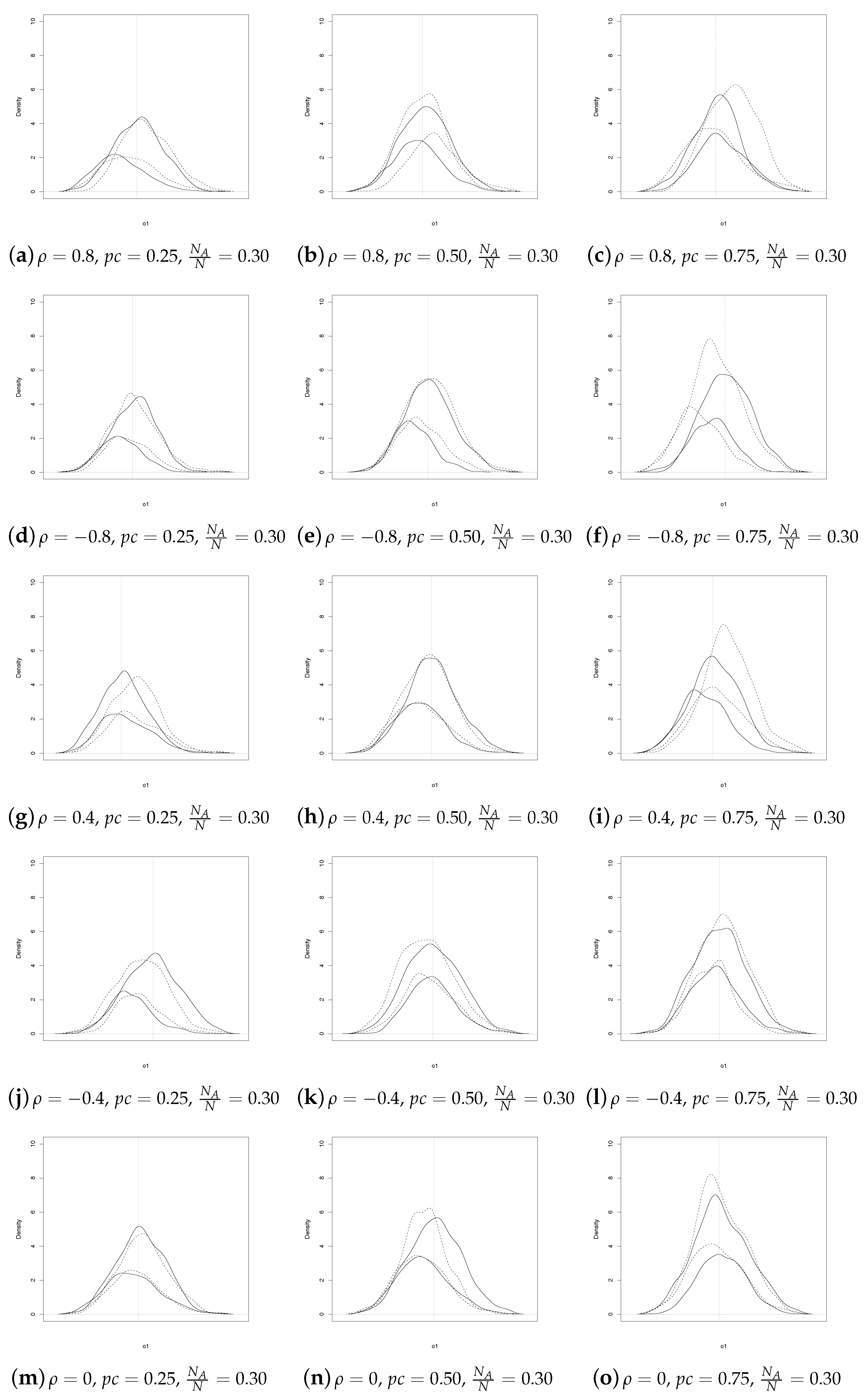
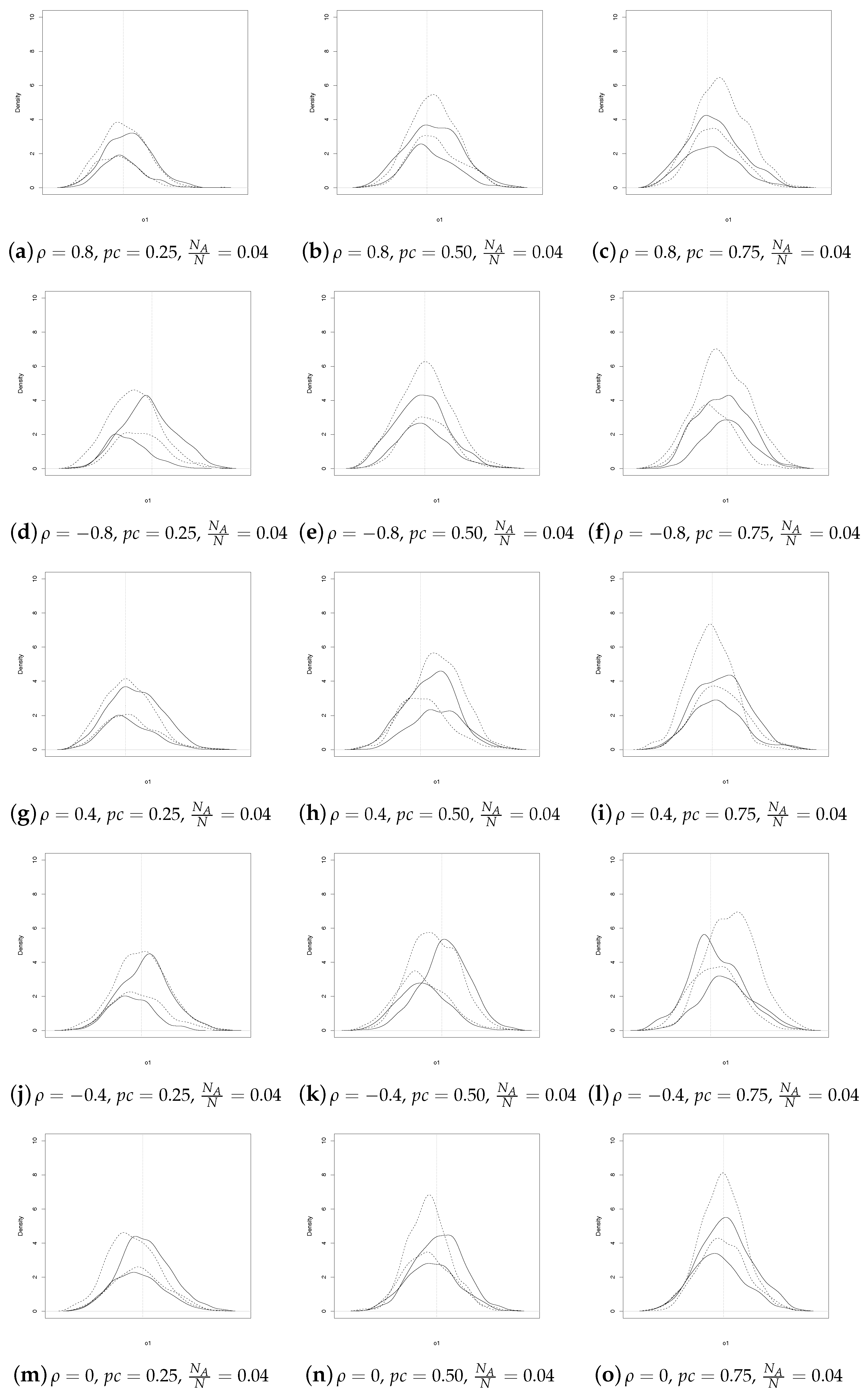
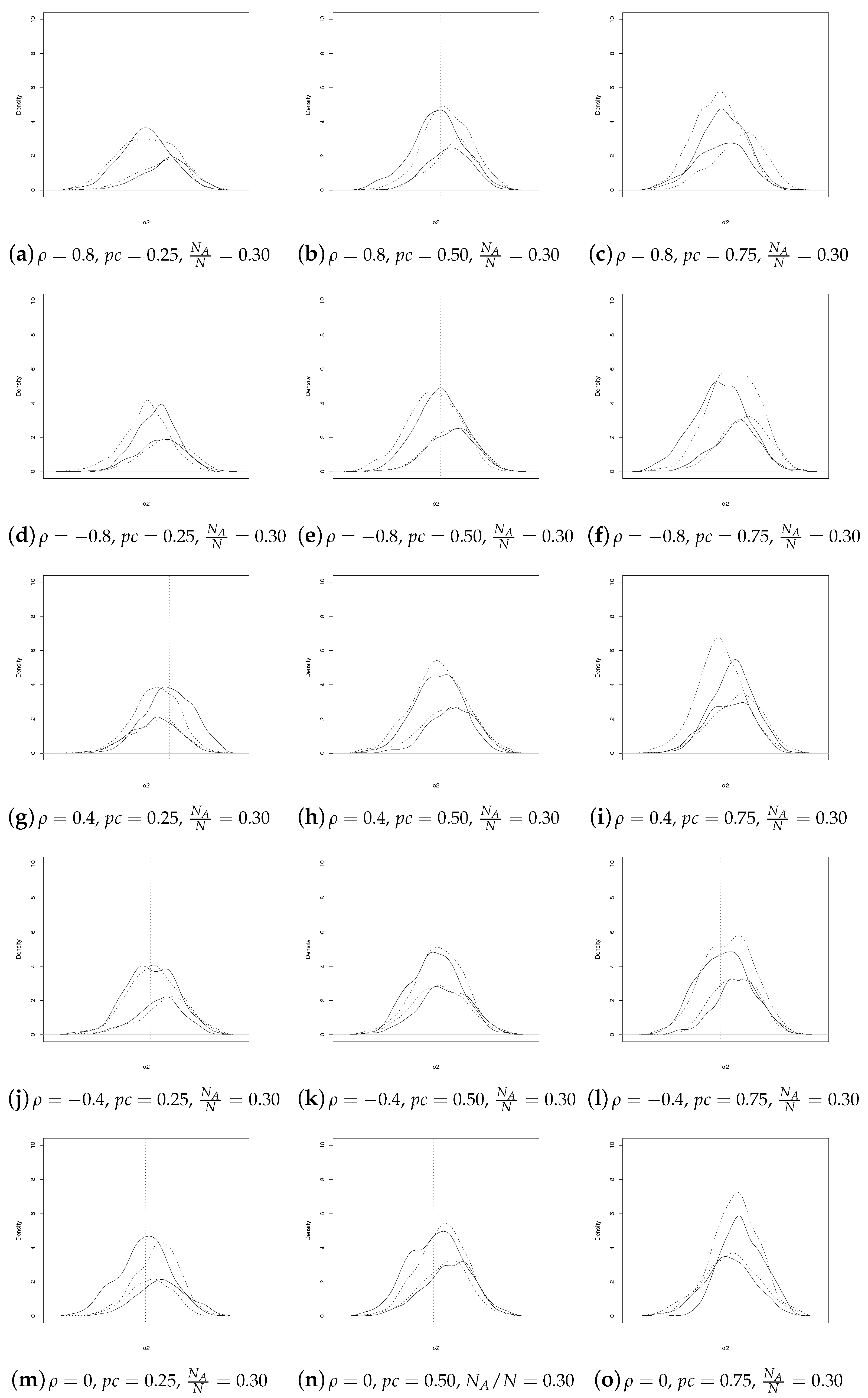
In commenting on the results, we begin by comparing the empirical densities of SSRS and GE estimators for $n=2000$ and $n=\mathrm{10,000}$, for each censoring scheme1. Rather than overwhelm the reader with statistics, we prefer to present information in a summary graphical form.

As regards ${\beta }_1$, for $N_A/N=0.04$ (see Figure 1), we note that the patterns are similar for $pc=0.25$, whereas the behavior differs more as $pc$ increases. Furthermore, the SSRS estimator is almost always more concentrated except for few combinations of $\rho$ and $pc$.

As expected, when $N_A/N$ increases, the discrepancies between SSRS and GE estimators fade away (see Figure 2).

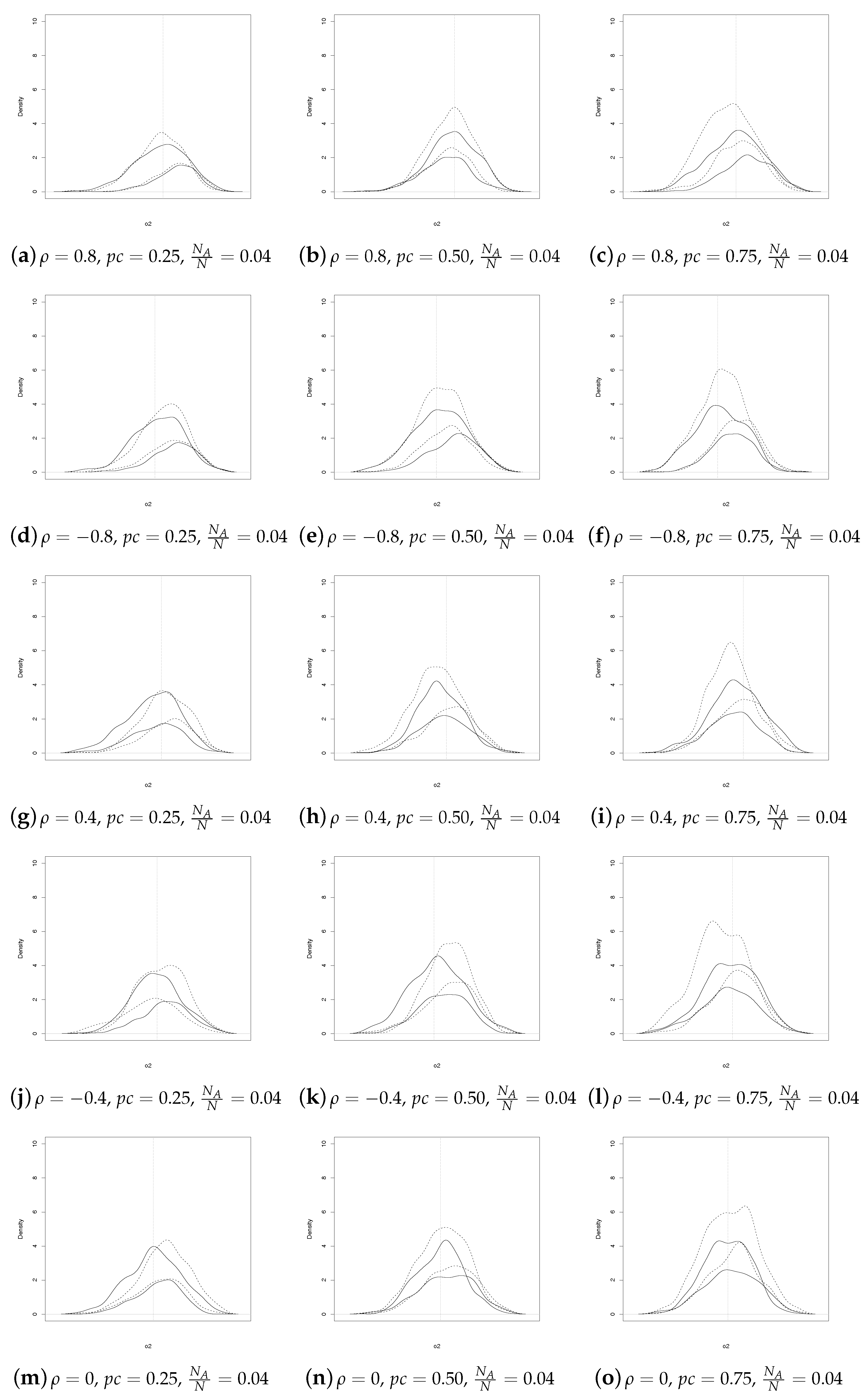
Analogous considerations apply for ${\beta }_2$ (see Figure 3 and Figure 4). In summary, Figure 1, Figure 2, Figure 3 and Figure 4 show that the SSRS and GE estimators have comparable behavior, even though the former uses less information at population level. It should be underlined that a direct comparison between the two sets of coefficient estimates may not always be appropriate. In fact, as noted by Mroz and Zayats (2008), a better comparison would be based on the relative effect, that is on the coefficients ratio. For these reasons we computed the average ratios ${\widehat{\theta }}_2/{\widehat{\theta }}_1$ and ${\widehat{\beta }}_2/{\widehat{\beta }}_1$ in the simulations, for each $k,pc,N_A/N$. The results, available upon request, are very close to the true ratios, ${\theta }_2/{\theta }_1=-0.63$ and ${\beta }_2/{\beta }_1=-1.2$, for both GE and SSRS estimators and they show once again that GE slightly outperforms SSRS in the selection equation, while the reverse seems to happen for the outcome equation.

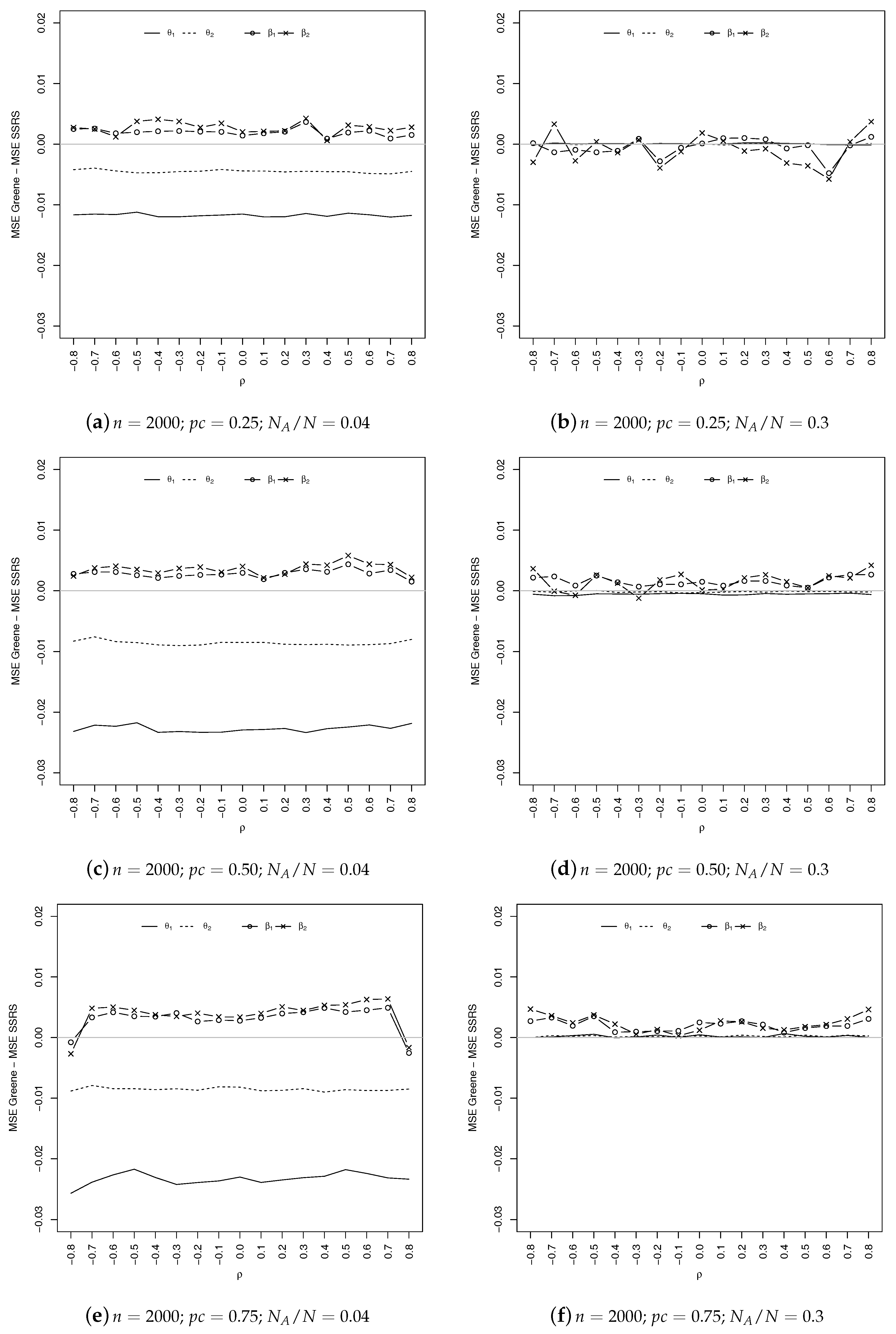
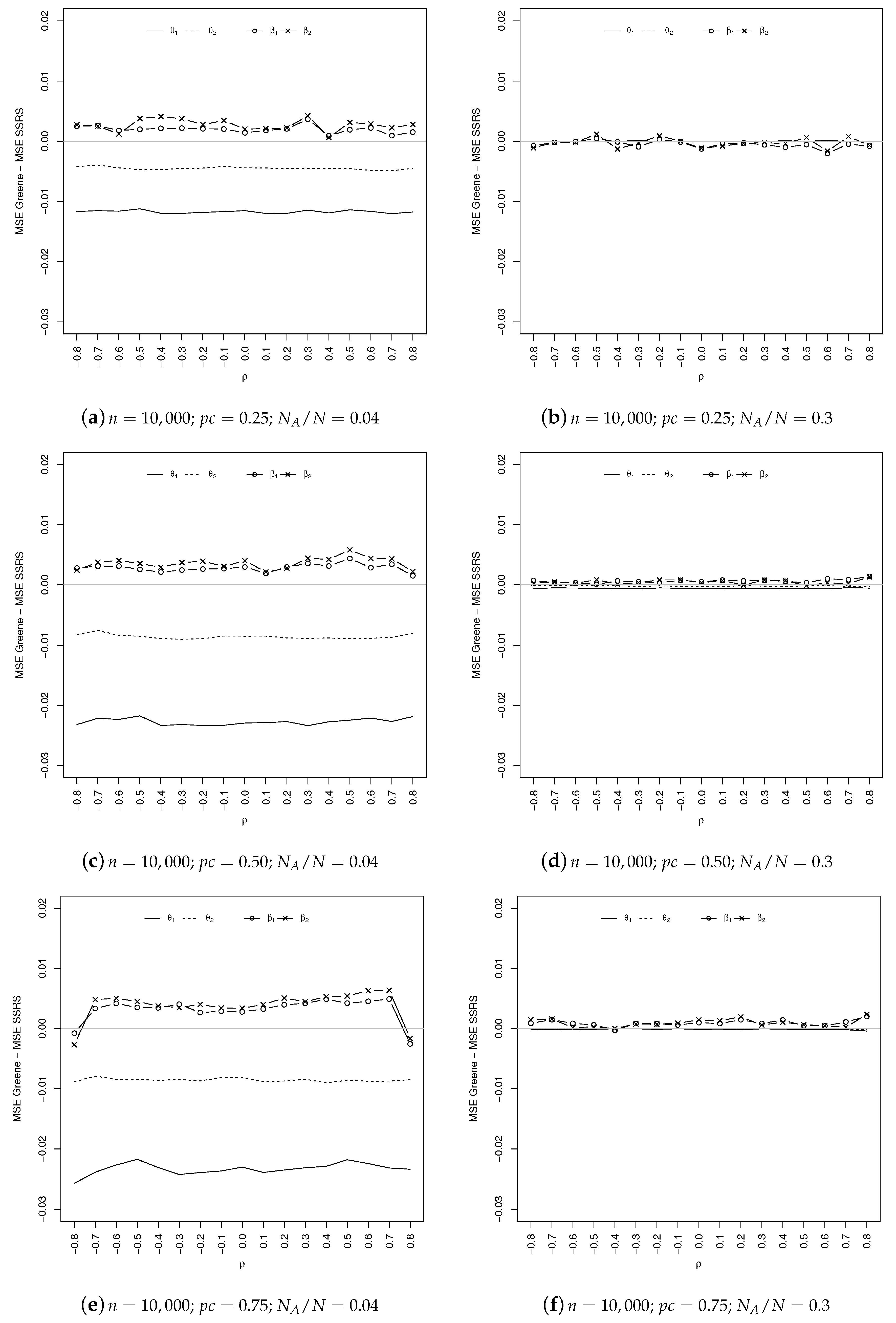
Coming to the comparison of the estimated MSEs, as shown in Figure 5 and Figure 6, the overall results obtained by the SSRS estimator are quite similar to Greene’s. Specifically, it seems that SSRS gives better results in estimating the parameters of the outcome equation (which are, generally speaking, those of greater interest), especially in the case of a severe censoring mechanism ($N_A/N=0.04$). The situation is reversed for the selection equation.

When $N_A/N=0.30$, the two estimators are substantially equivalent for the selection equation, while SSRS continues to slightly outperform GE for the outcome (except for $pc=0.25$).

As expected, when $N_A/N$ increases, the differences between the MSEs of the two estimators decrease in absolute value. Everything we said holds for both sample sizes.

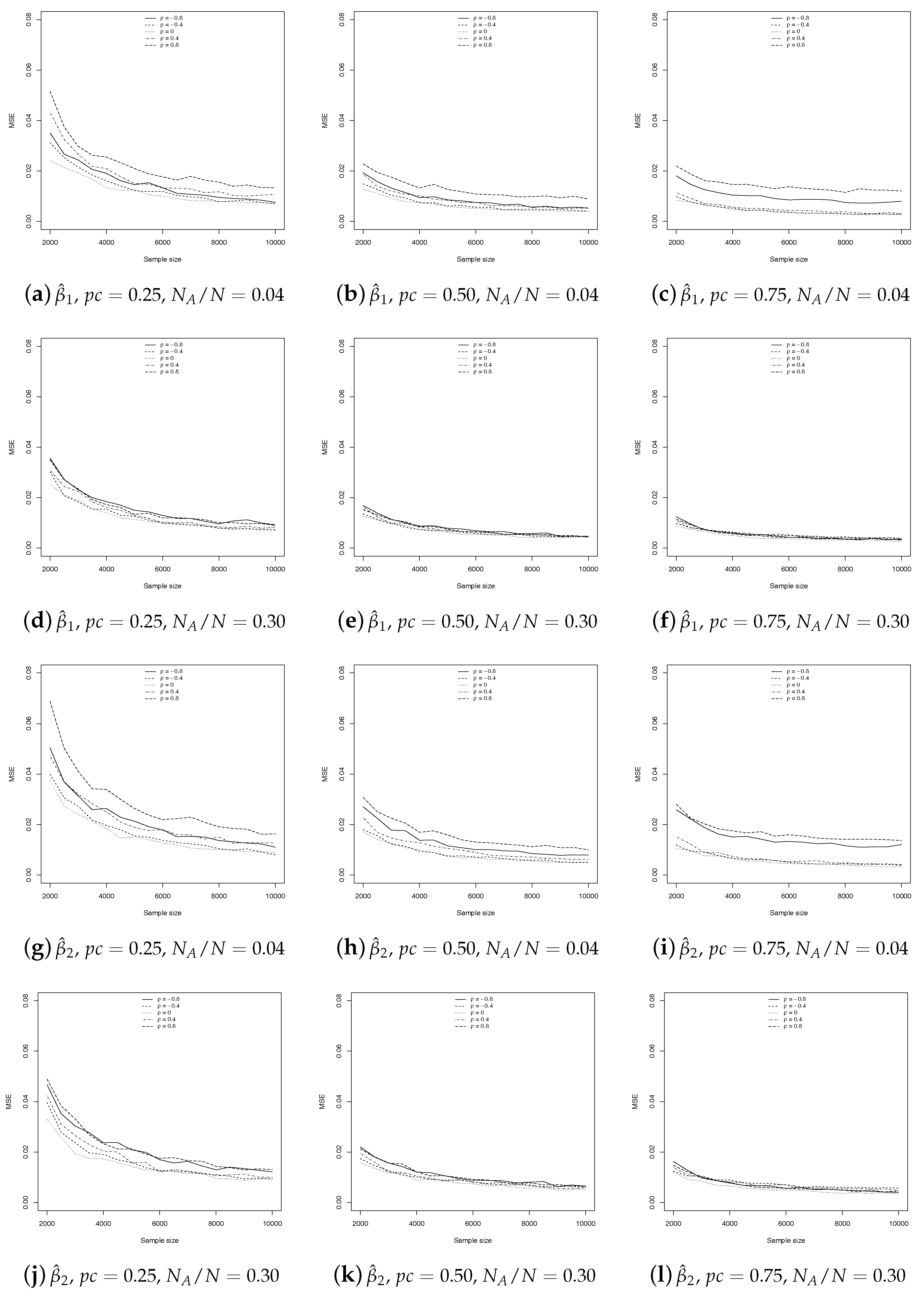
Finally, in Figure 7, we present the trend of the MSEs as the sample size increases, to have a first idea of the possible consistency of our estimator. Clearly, the property of consistency can only be proven analytically. The evaluation has been made only for the SSRS estimator, as it is proven that GE is consistent (Greene 2008; Manski and Lerman 1977). As usual, we consider the three sampling percentages and we compute the MSE for ${\widehat{\beta }}_1$, ${\widehat{\beta }}_2$, ${\widehat{\theta }}_1$ and ${\widehat{\theta }}_2$. Once again, to save space, we present only the former, but all are available upon request.

As suggested by a referee, we made further simulations to study the behavior of the two estimators when the true generating model of the disturbances is not normal, while the likelihood function is based on the probabilities specified in Equations (9)–(11) (normal distribution). In particular, the generating model considered here is a bivariate skew-T; we then simulated 500 samples of size $n=2000$ and $n=\mathrm{10,000}$, $\rho \in 0,\pm 0.4,\pm 0.8$, $pc\in 0.25,0.50,0.75$ and $N_A/N\in 0.04,0.15,0.30$. The behavior of the two estimators remains comparable in terms of bias and mean square error. In particular, comparing the mean square errors, GE outperforms SSRS in the estimation of the selection equation; the situation is often reversed for the outcome equation. Furthermore, to compare the robustness to distribution mispecification of the two estimators, we computed the ratio between the bias obtained when the true generating model is a skew-T and the bias obtained when the model is correctly specified: the closer to one the ratio (in absolute value), the more robust the estimator. It emerges that the SSRS estimator is more robust than GE, especially for the selection equation parameters. All results are available upon request.

4. Application on Real Data: Estimation of Credit Scoring

In the following, we consider the problem of estimating the risk of a loan default for credit-card holders. The population of interest is that of loan applicants, for whom some requests are approved and some are rejected according to their loan default risk.

The idea is to use the model to assign a default probability to a random individual who applies for a loan, but the only information that exists about default probabilities comes from previous loan recipients. The problem is that the probability of default for the overall population of applicants is not necessarily the same as for those who have already received a credit card (in fact, we expect that the probability for the whole population is greater than that of cardholders). To avoid this kind of selection bias, we need to consider the selection mechanism explicitly, that is a selection equation which explains the cardholder status.

The dataset considered here2 contains a subset of the covariates used in Greene (2008). On $n=\mathrm{13,444}$ cardholders, the following characteristics are measured: cardholder status (CH), taking 1 if the application for a credit card was accepted and 0 if not; default status (D), taking 1 if defaulted and 0 if not (observed only when CH = 1, that is for 10,499 observations); age in years plus twelfths of a year (Age); number of dependents (Adepcnt); months living at current address (Acadmos); number of major derogatory reports (Mjrg); number of minor derogatory reports (Mndrg); owner or tenant (Ownrent), taking 1 if the applicant owns his/her home, 0 if renting; monthly income in US dollars divided by 100 (Income); self employment status (Selfempl), taking 1 if self employed, 0 if not; and ratio of monthly credit card expenditure to yearly income (ExpInc).

We used the following specification:

$$\begin{array}{c}{D}_i={\beta }_0+{\beta }_{1}Adepcn{t}_i+{\beta }_{2}Incom{e}_i+{\beta }_{3}ExpIn{c}_i+{ϵ}_{1i}\\ C{H}_i={\theta }_0+{\theta }_{1}Incom{e}_i+{\theta }_{2}Ownren{t}_i+{\theta }_{3}Acadmo{s}_i+{\theta }_{4}Selfemp{l}_i+{\theta }_{5}Mjdr{g}_i+{\theta }_{6}Mndr{g}_i+{ϵ}_{2i}\end{array}$$

and we estimated the parameters by SSRS and GE estimators. The results, shown in

Table 1. Parameter estimates.

SSRS				GE
	beta	se	pval		beta	se	pval
Age	0.047	0.002	0.000	Age	−0.006	0.001	0.000
Income	−0.002	0.001	0.067	Income	0.018	0.001	0.000
Ownrent	0.039	0.031	0.208	Ownrent	−0.372	0.026	0.000
Acadmos	−0.002	0.000	0.000	Acadmos	0.002	0.000	0.000
Selfempl	0.005	0.060	0.928	Selfempl	0.216	0.045	0.000
Mjdrg	−0.440	0.013	0.000	Mjdrg	−0.385	0.013	0.000
Mndrg	0.393	0.019	0.000	Mndrg	−0.164	0.016	0.000
Cons	−0.144	0.052	0.005	Cons	−0.166	0.042	0.000
Adepcnt	0.430	0.014	0.000	Adepcnt	0.059	0.017	0.001
Income	−0.070	0.002	0.000	Income	−0.012	0.002	0.000
ExpInc	−0.153	0.157	0.329	ExpInc	0.170	0.181	0.349
Cons	−0.048	0.050	0.342	Cons	−0.562	0.050	0.000

, are quite similar for the outcome equation (the one of greater interest because it gives the credit scoring), where the signs are coherent with expectations.

To evaluate the predictive performance of the two models, we computed the confusion matrices (see

Table 2. Confusion matrices: observed vs predicted for non cardholders ($\overline{CH}$), non defaulted ($CH\cap \overline{D}$) and defaulted ($CH\cap D$).

	SSRS	Predicted
		$\overline{CH}$	$CH\cap \overline{D}$	$CH\cap D$
Observed	$\overline{CH}$	484	2302	159
	$CH\cap \overline{D}$	58	9210	235
	$CH\cap D$	6	947	43
	GE	Predicted
		$\overline{CH}$	$CH\cap \overline{D}$	$CH\cap D$
Observed	$\overline{CH}$	2747	198	0
	$CH\cap \overline{D}$	7984	1519	0
	$CH\cap D$	897	99	0

), which allowed us to compute the percentages of correct predictions.

From these matrices, it is easy to obtain the percentages of correct predictions for both estimation procedures. In particular, the overall percentages are 0.724 and 0.317 for SSRS and GE, respectively, showing a strong dominance of the former estimation method over the latter. This dominance is even more evident in the percentages conditioned on the default status: for non defaulters, the percentage is 0.969 for SSRS and 0.160 for GE, while, for defaulters, it is 0.043 for SSRS and 0 for GE. On the other hand, GE outperforms SSRS in the prediction of non cardholder status: the values are 0.164 for SSRS and 0.933 for GE.

5. Conclusions

In this paper, we propose a method for estimating the regression coefficients in binary response models with sample selection, when a censoring mechanism intervenes to make a vast majority of units unobservable. We derive the likelihood function analytically, taking advantage of the response-based sampling framework and find that it is a weighted version of Heckman’s likelihood.

A simulation study highlights that the finite sample performance of the point estimators are very satisfactory even when compared to a similar estimator (Greene 2008), which in turn assumes knowledge of the population proportion of occurrences in the outcome equation. Specifically, our estimator slightly outperforms Greene’s in estimating the parameters of the outcome equation (which are, generally speaking, those of greater interest), especially in the case of a severe censoring mechanism ($NA/N=0.04$). Under this censoring scenario, the situation is reversed for the selection equation. When the censoring is less severe, the two estimators are substantially equivalent for the selection equation, while in general ours still outperforms Greene’s for the outcome.

An analogous result is obtained in an empirical analysis aimed to estimate the risk of loan default: our estimator performs better in the prediction of the dependent variable of the outcome equation (i.e., the default status), while Greene’s does better in the selection equation (i.e., the prediction of the cardholder status).

The fact that the best results refer to the outcome equation is an advantage, since it is generally the one of greater interest. The main result is that we do not require knowledge of the true prevalence of occurrences, that is, our estimator can be successfully used when $N_{1A}\mathrm{and}{N}_{0A}$ are unknown.

Future research will be devoted to the problems arising from measurement errors, either in the dependent variable or in the covariates of the outcome equation. In the first case, the problem is obviously simpler and a modified version of the likelihood can take into account the bias arising from this kind of error. In the second case, an endogeneity issue arises and it is necessary to consider further information, for example, instrumental variables.