Time-Varying Window Length for Correlation Forecasts

Abstract

Forecasting correlations between stocks and commodities is important for diversification across asset classes and other risk management decisions. Correlation forecasts are affected by model uncertainty, the sources of which can include uncertainty about changing fundamentals and associated parameters (model instability), structural breaks and nonlinearities due, for example, to regime switching. We use approaches that weight historical data according to their predictive content. Specifically, we estimate two alternative models, ‘time-varying weights’ and ‘time-varying window’, in order to maximize the value of past data for forecasting. Our empirical analyses reveal that these approaches provide superior forecasts to several benchmark models for forecasting correlations.

1. Introduction

Variance and covariance (or correlation) estimates are important inputs for many decisions, including pricing derivatives, risk measurement, risk management and asset allocation or investment decisions. For instance, Andersen et al. (2007) discuss how the realized covariance matrix is useful in risk management applications. On the investment side, Fleming et al. (2003) study how using realized variance can improve a volatility-timing strategy, while Bandi et al. (2008) focus on the optimal portfolio choice problem using the realized covariance matrix. Furthermore, Corsi et al. (2013) and Christoffersen et al. (2014) show that using realized variance improves option pricing performance.

Therefore, accurate forecasting of the covariance matrix is important. Forecasting is fraught with potential biases and inefficiencies arising from model uncertainty, the sources of which can include uncertainty about changing fundamentals and associated parameters (model instability), structural breaks and nonlinearities due, for example, to regime switching. Applying a best-practice structural model from finance theory will usually require a long history of data for precise estimates of model parameters. Due to model instability, many forecasters use a nonparametric filter based on a fixed-length moving window of observable returns, for example, an exponentially-weighted moving average. However, the question remains: Over what historical sample should the sample average or the moving-average forecasts be computed? Given model uncertainty or instability, forecasters require some way of deciding what data sample to use.

The forecasting efficacy of time series models of realized variance has a very extensive literature.1 In this paper, we focus on forecasting correlations of stock returns with commodities. Correlations between stock returns and commodities are particularly important since they measure how much diversification benefit can be achieved by investing across different asset classes. The extant literature has been mainly focused on whether the co-movements between stocks and commodities have been steadily increasing since the financialization of commodities markets. Depending on their empirical setup, there is evidence showing that correlations between the two markets have increased; but also evidence showing that the impact of financialization is not transparent.2

Either way, it is clear that the time series of variances and correlations between stocks and commodities exhibit frequent shifts. For example, the average daily realized correlation between S&P500 futures and gold futures was 0.16 for the period April 2007–February 2015; but −0.38 and 0.54 for the subperiods July 2008–August 2008 and January 2010–February 2010, respectively. This feature makes forecasting challenging. Using a longer data sample does not necessarily lead to better forecasts and can possibly introduce additional bias. On the other hand, using a fixed-length moving window requires some method of selecting the best window length. Motivated by this challenge, we focus on comparing alternative data usage models, time-varying weights and time-varying window lengths, in order to maximize the predictive content of historical data.

Breaks in conditioning information or model uncertainty have typically been addressed with respect to forecasting returns.3 The recognition that predictor variables are imperfect or uncertain can result in returns being riskier in the long-run than the short-run due to that model uncertainty.4 Structural break models provide similar intuitions although they are typically less frequent than the model changes we allow for in this paper.5 More directly related to our approach is the optimal window-width literature; for example: (Pesaran and Timmermann (2002); Pesaran and Timmermann (2007)) with respect to returns; and Härdle et al. (2014) with respect to trading volumes.

Since forecasts are often sensitive to the data sample used to derive the forecast, an approach that can use historical data optimally (with respect to predictive content) at each point in time should provide superior real-time forecasts. One such approach is a Bayesian model of learning about model change as new data arrive. We evaluate two alternatives to the typical benchmarks of a fixed-length moving window or an expanding window that weights historical data equally.

Our first alternative, a ‘time-varying weights’ model, estimates weights for data histories according to their out-of-sample predictive content. Following Maheu and Gordon (2008) and Maheu and McCurdy (2009), historical data are partitioned into submodels, which have different data histories. Submodel probabilities are estimated each period based on predictive content. Bayesian model average forecasts for each period combine an estimated model change probability with a probability-weighted average of submodel forecasts, integrating-out submodel uncertainty. In this case, the forecasted distributions of realized variances and realized correlations are generated by discrete mixtures of submodel distributions, using information from all of the submodels, appropriately weighted by the estimated submodel probabilities. In other words, all of the data are used for generating forecasts but rather than weighting the submodels equally (cf., Pesaran and Pick 2011), our submodel weights are estimated each period according to how useful those data are for the forecasts. In terms of the bias versus efficiency issue, when there is a change in the data-generating process, this approach will use data prior to a probable model change if those data improve the forecast.

Our second alternative is a ‘time-varying window’ model. This approach builds on the ‘time-varying weights’ model by truncating the data history, every period, at the point of most mass for the submodel probability distribution. We redo our forecasts using this time-varying window length. This alternative approach provides a further interesting comparison with the fixed-length moving window benchmark, as well as with the time-varying weights approach, which assesses the usefulness of all data histories and weights them accordingly, period by period. It also allows a further analysis of the bias versus efficiency issue.

We compare our time-varying weights and time-varying window forecasts to standard benchmark forecasts. Our first benchmark, motivated by the conclusion of Welch and Goyal (2008) for forecasting returns, is the sample average of realized variances and realized correlations based on an expanding window as new data arrive. Our second benchmark, motivated by industry practice, is the moving average associated with a fixed-length moving window. Further, since our method is not dependent on any particular statistical model, but rather evaluates the usefulness of alternative samples of historical data, we provide several robustness checks for the forecasting efficacy of the time-varying weights and time-varying window approaches. These include long-horizon forecasts, as well as exponentially-weighted moving average and AR(1) forecasting models. Our approach is equally applicable to more advanced conditional forecasting models such as HAR (Heterogeneous Auto-Regressive) model (Corsi 2009). However, our focus is on the time-varying usage of the historical data rather than specific statistical models.

Our empirical analyses for forecasts of variances and correlations between stocks and commodities reveal that both the time-varying weights and time-varying window approaches provide much superior forecasts than fixed-length moving window and expanding window models that weight historical data equally. Our result is also strong for long-horizon forecasts. The time-varying weights model dominates for all cases according to the log-likelihood metric for forecasting the distributions of realized variances and realized correlations. On the other hand, the time-varying window-length model dominates when evaluating forecasts of realized variances and realized correlations using mean absolute error, average sum of squared errors and $R^2$ metrics from forecast regressions. Our comparisons with alternative benchmarks, in particular, exponentially-weighted moving-average and AR(1) forecasting models, show that optimizing with respect to historical data usage adds value relative to those alternatives, as well.

The rest of the paper is organized as follows. The next section describes the high-frequency data sources and construction of realized measures. Section 3 and our Appendix are devoted to detailed descriptions of our model, estimation and deriving forecasts. Estimation results and forecast accuracy are discussed in Section 4. Section 5 performs various robustness checks, and Section 6 concludes.

2. Data

In this section, we discuss the data and describe how we constructed the variables, which are the focus of our forecasts. We will focus on various realized variance RV and realized correlation RCorr measures in this paper, although our approach can be applied to general datasets.

For each period, assume that we have L number of intra-period returns available. Using the notation $r_{i;t,l}$ to denote continuously-compounded return of security i at time t and intra-period l, we construct the realized variance measure of security i over period t as follows.

$$\begin{array}{c}\hfill R{V}_{i,t}=\sum _{l=1}^L{r}_{i;t,l}^2\end{array}$$

(1)

It is well known that empirically-observed intra-period returns exhibit serial autocorrelations. This violates the assumption that guarantees the consistent convergence of the above formula to the actual variance. Thus, we follow Hansen and Lunde (2006) to make a kernel adjustment:

$$\begin{array}{ccc}\hfill R{V}_{i;t,A{C}_q}& =& {\omega }_0\widehat{{\gamma }_0}+2\sum _{j=1}^q{\omega }_j\widehat{{\gamma }_j};\hfill \end{array}$$

(2)

$$\begin{array}{ccc}\hfill \widehat{{\gamma }_j}& =& \sum _{l=1}^{L-j}{r}_{i;t,l}{r}_{i;t,l+j}\hfill \end{array}$$

(3)

using the Bartlett scheme to define weights, so that ${\omega }_j=1-\frac{j}{q+1},j=0,1,\dots ,q$.

Our first dataset consists of monthly realized variances from February 1885–December 2013 inclusive. The early part of the sample from 1885–1925 uses daily returns from Schwert (1990). Daily returns from January 1926 forward were obtained from the Center for Research in Security Prices (CRSP) for the S&P500 index (and earlier representations of that index). The number of lags q used to adjust for intra-period serial autocorrelation was chosen to be three. This gives us 1543 months of RV data for the U.S. equity market.

Our next dataset uses intraday returns data from futures markets to construct daily RV measures. Starting from April 2007 and ending in February 2015, we obtained intraday futures prices for S&P 500 futures with trading symbol SP on the CME (Chicago Mercantile Exchange) , for COMEX (Commodity Exchange, Inc.) gold futures with trading symbol GC on the COMEX and for light crude oil futures with trading symbol CL on the NYMEX (New York Mercantile Exchange) . These intraday prices are from TickData at a 15-min frequency.6 We will use the trading symbol of each futures price to denote them for the remainder of this paper.

The first measure of interest is the daily realized variance of these three futures. Using the same steps as above, we compute daily RV using the 15-min continuously-compounded returns. We again adjust for possible intraday autocorrelations using the Bartlett scheme. A 15-min grid was chosen to minimize any effect coming from microstructure noise. This yields 2050 observations of daily RV for each of the three futures.

Our next measure of interest is daily realized correlations, RCorr, for the three futures contracts. Using the cross-product of intraday returns at the same 15-min frequency, we first construct a daily realized covariance between security i and j, denoted by $RCo{v}_{i,j,t}$, as follows:

$$\begin{array}{c}\hfill RCo{v}_{i,j,t}=\sum _{l=1}^L{r}_{i;,t,l}{r}_{j;,t,l}.\end{array}$$

(4)

Then, the daily realized correlation between security i and j is constructed in the usual manner:

$$\begin{array}{c}\hfill RCor{r}_{i,j,t}=\frac{RCo{v}_{i,j,t}}{\sqrt{R{V}_{i,t}R{V}_{j,t}}}.\end{array}$$

(5)

Lastly, for the ease of estimation, we will work with transformations of these realized measures. It is well-known that the log of realized variance closely follows a normal distribution (Andersen et al. 2001). Similarly, the Fisher transformation of realized correlations also closely follows a normal distribution. Therefore, we will work with the following set of variables in the estimation section:

$$\begin{array}{ccc}\hfill log{\mathit{RV}}_{i,t}& =& log({\mathit{RV}}_{i,t})\hfill \end{array}$$

(6)

$$\begin{array}{ccc}\hfill Fis{\mathit{RCorr}}_{i,j,t}& =& 0.5log(\frac{1+{\mathit{RCorr}}_{i,j,t}}{1-{\mathit{RCorr}}_{i,j,t}})\hfill \end{array}$$

(7)

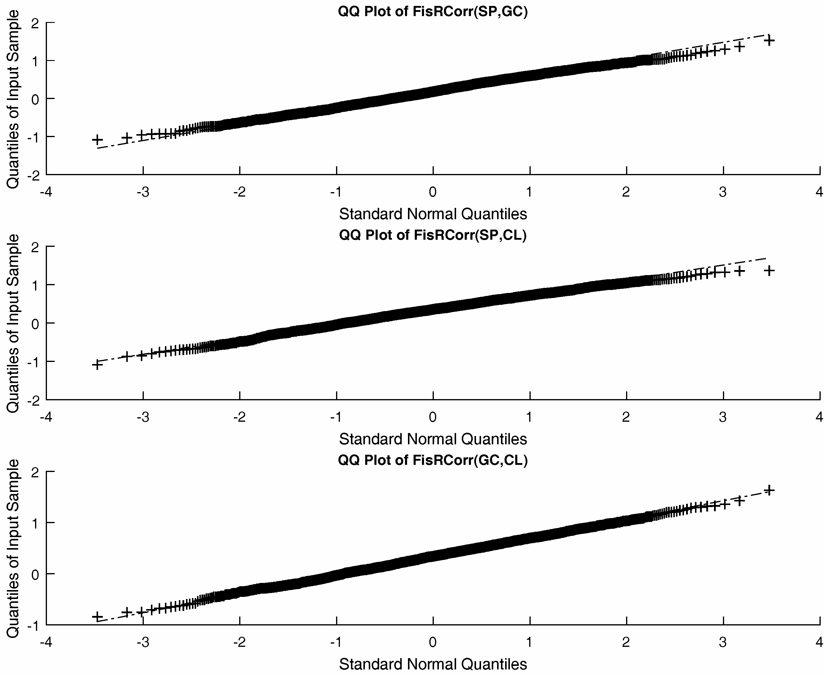
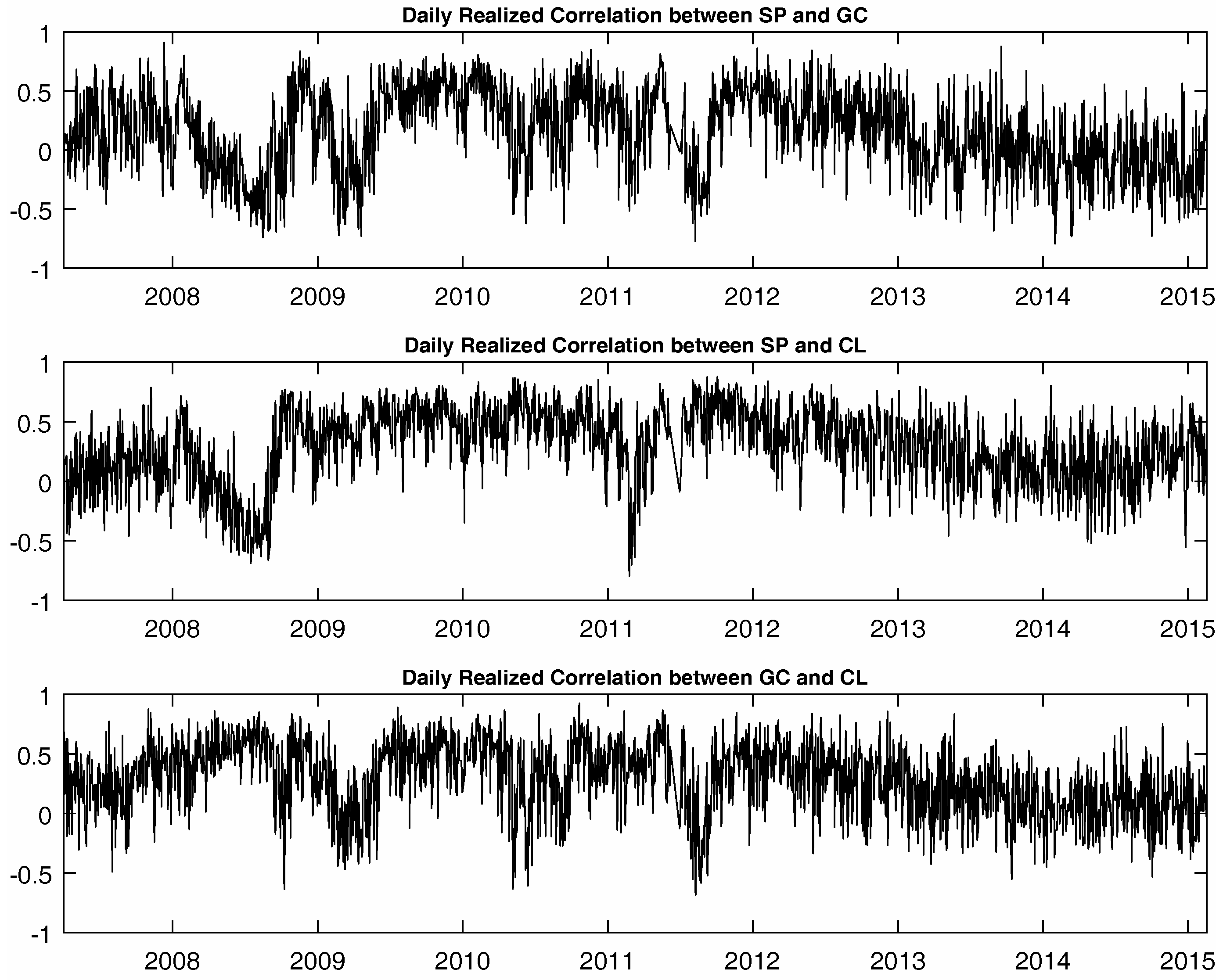
Three time series of daily realized correlations between futures pairs are plotted in Figure 1. The plots illustrate the fact that these daily realized correlations are highly time-varying and nowhere close to being constant, thus making the effort to model and predict them worthwhile. To verify the validity of our normality assumptions,

Table 1. Summary statistics for realized measures.

Symbol	Mean	Variance	Skewness	Kurtosis
Panel A: Summary Statistics for Realized Variances
Monthly Frequency, Sample Period 1885–2013
logRV (S&P)	−6.5229	0.9012	0.7168	4.1608
RV (S&P)	0.0026	2.45E-05	6.2809	54.4785
Daily Frequency, Sample Period April 2007–February 2015
logRV (SP)	−10.3408	1.7155	0.3836	3.8697
logRV (GC)	−10.6170	1.4464	0.2023	3.3387
logRV (CL)	−9.1946	1.4406	0.2025	3.3763
RV (SP)	9.34E-05	7.91E-08	9.2736	118.6787
RV (GC)	5.51E-05	2.03E-08	14.8284	325.9368
RV (CL)	2.23E-04	1.86E-07	6.0766	57.7090
Panel B: Summary Statistics of Realized Correlations
Daily Frequency, Sample Period April 2007–February 2015
FisRCorr (SP, GC)	0.1806	0.1656	−0.0773	2.6457
FisRCorr (SP, CL)	0.3398	0.1438	−0.2480	2.9505
FisRCorr (GC, CL)	0.3338	0.1288	−0.0292	2.8818
RCorr (SP, GC)	0.1570	0.1255	−0.2723	2.2468
RCorr (SP, CL)	0.2952	0.1011	−0.6201	2.8742
RCorr (GC, CL)	0.2912	0.0904	−0.4602	2.6393

Notes: This table provides summary statistics of realized measures constructed from high-frequency data. The top panel shows the descriptive statistics of realized variance measures, and the bottom panel shows the descriptive statistics of realized correlation measures. We compute monthly realized variance (RV) of the S&P index using the daily returns data from 1885–2013. Daily realized variances and correlations for three futures contracts written on the S&P500 index, gold and light crude oil are computed using the 15-min grid of changes in log futures prices from TickData beginning 2 April 2007 and ending 17 February 2015. We use symbols SP, GC and CL to denote the S&P500 index, gold and light crude oil futures, respectively. We apply the kernel adjustment of Hansen and Lunde (2006).

reports descriptive statistics for logRV and Fis RCorr. Without loss of generality, we can safely make an assumption that these variables are normally distributed as evidenced by skewness and kurtosis values in the last two columns. Figure 2 also provides QQ-plots for FisRCorr, which again verifies that the normality assumption is not too strong for these transformed variables.

3. Model

Following Maheu and Gordon (2008) and Maheu and McCurdy (2009), a key ingredient of our modelling approach is submodels that correspond to different data histories. In this section, we describe how submodels are defined for our application and discuss how we estimate them.

3.1. Submodels

As shown in the previous section, it seems reasonable to assume that the unconditional distributions of logRV and FisRCorr are Gaussian. Henceforth, we assume that the dataset of interest, denoted by $x_t$ from here on, follows a Gaussian distribution.

Suppose that one has a specific model in mind that she/he believes to describe $x_t$. In order to make a forecast for next period t at time $t-1$, one needs to decide how much data history to use to calibrate the model parameters. Intuitively, it sounds reasonable to use the entire dataset available at time $t-1$. In other words, one can use all observed data points $\{x_1,\dots ,x_{t-1}\}$. However, one can also question whether information contained in early parts of the sample are useful, and sometimes even harmful, for forecasts. For example, the underling data-generating process may not be stable over time, but rather may experience frequent model changes with respect to its parameters. In this case, including the old observations will introduce a bias. Therefore, wisely choosing the optimal window of data history becomes a critical issue when there are possible frequent model changes throughout time.

This motivates us to define submodels indexed by the starting point of a data history for calibration. Let $\mathit{\theta }$ denote the set of parameters of the specific model we would like to estimate. The notation $M_{\tau }$ denotes a submodel that uses data history starting from $\tau$ to the time $t-1$. Hence, at time $t-1$, $M_1$ denotes a submodel that uses the entire data history $\{x_1,\dots ,x_{t-1}\}$; $M_2$ denotes a submodel that disregards the first observation and uses $\{x_2,\dots ,x_{t-1}\}$; and $M_{\tau }$ denotes a submodel that uses $\{x_{\tau },\dots ,x_{t-1}\}$. Each submodel represents a possible model change in the underlying data generating process. When a model change in the underlying data-generating process occurs, data prior to the change can introduce a bias to the estimation if included. Therefore, it becomes more informative to use a partial dataset starting from the date of the model change.

Obviously, we cannot identify exactly where the model change occurs. We can only infer the probability of each model being the right one based on its predictive content. This is the key intuition of our approach, which we discuss in the next subsection.

3.2. Combining Submodels

In this subsection, we discuss how to combine and estimate the probabilities associated with each submodel. As submodel probabilities are chosen to maximize the predictive density at each time t, we will follow a recursive procedure to update probabilities as time progresses.

For convenience, we first introduce the following notation for the information set generated by observations between time periods a and b:

$$\begin{array}{c}\hfill {\Omega }_{a,b}\equiv \left\{\begin{array}{cc}\mathbb{I}\{x_a,\dots ,x_b\}\hfill & \mathrm{if}a\le b\hfill \\ \{\varnothing \}\hfill & \mathrm{if}a>b.\hfill \end{array}\right.\end{array}$$

(8)

Using this notation, we write the predictive density of $x_t$ at time $t-1$ given the parameter vector $\mathit{\theta }$ under the submodel $M_{\tau }$ as $p(x_t|{\Omega }_{\tau ,t-1},\mathit{\theta },M_{\tau })$. Recall that the submodel $M_{\tau }$ assumes that any data prior to time $\tau$ contain no signal. Therefore, conditioning on the submodel $M_{\tau }$ effectively becomes using the information set ${\Omega }_{\tau ,t-1}$ to build the predictive density.

To compute the predictive density associated with $x_t$ under the submodel $M_{\tau }$, we need to integrate out the uncertainty associated with the parameter vector $\mathit{\theta }$ as below:

$$\begin{array}{c}\hfill p(x_t|{\Omega }_{\tau ,t-1},M_{\tau })=\int p(x_t|{\Omega }_{\tau ,t-1},\mathit{\theta },M_{\tau })p(\mathit{\theta }|{\Omega }_{\tau ,t-1},M_{\tau })d\mathit{\theta }.\end{array}$$

(9)

We will discuss how to implement the first term inside the above integral in the next section. Meanwhile, the second term inside the above integral is effectively the posterior distribution of the parameter vector under the submodel $M_{\tau }$. Following the usual Bayes’ rule with the notation $p(\mathit{\theta }|M_{\tau })$ to denote the prior distribution of the parameter vector associated with the submodel $M_{\tau }$, we have:

$$\begin{array}{c}\hfill p(\mathit{\theta }|{\Omega }_{\tau ,t-1},M_{\tau })\propto \left\{\begin{array}{cc}p(x_{\tau },\dots ,x_{t-1}|\mathit{\theta },M_{\tau })p(\mathit{\theta }|M_{\tau })\hfill & \mathrm{if}\tau <t\hfill \\ p(\mathit{\theta }|M_{\tau })\hfill & \mathrm{if}\tau =t\hfill \end{array}\right.\end{array}$$

(10)

That is, if $\tau$ is less than t, we only use the data starting from time $\tau$ up to $t-1$ to update our belief on the parameter vector. If $\tau$ is equal to t, then we have no information to rely on to update our belief, and thus, the posterior is equal to the prior.

Having established the predictive density associated with each submodel, we now turn to discuss how to combine the submodels recursively over time and how to estimate the submodel probabilities. Recall that our intuition builds upon the assumption that there is a chance at each time t that past data become uninformative. In order to rigorously model this intuition, we introduce the process ${\lambda }_t$ to describe the probability of past data becoming uninformative at each time t. In other words, at each time t, there is ${\lambda }_t$ probability that the data prior to time t are no longer useful and will only distort the prediction. As we discussed earlier, this can be due to many reasons including the model changes in the underlying data generating process.

To introduce the idea, we first limit our discussion to the case where ${\lambda }_t$ is deterministic and known. In the next section, we will extend to the case where ${\lambda }_t$ is stochastic and also needs to be estimated. For convenience, we use the notation ${\Lambda }_t=\{{\lambda }_2,\dots ,{\lambda }_t\}$ to refer to the set of probabilities ${\lambda }_t$ up to time t. Note that since model change at Time 1 does not mean anything, we let ${\Lambda }_1$ be the empty set.

Let us begin from time $t=0$. At this point, we do not have any observations so the predictive density of $x_1$ is simply its normally distributed prior belief $p(x_1|{\Omega }_{0,0},M_1)$. We will discuss below how hyperparameters are set for the prior belief. Now, at time $t=1$, we have one observation $x_1$. We have two cases to consider now. That is, past data can either be useful or become uninformative at Time 2, which will happen with probability ${\lambda }_2$. This allows us to write the predictive density of $x_2$:

$$\begin{array}{c}\hfill p(x_2|{\Omega }_1,{\Lambda }_2)=p(x_2|{\Omega }_{1,1},M_1)p(M_1|{\Omega }_1,{\Lambda }_1)(1-{\lambda }_2)+p(x_2|{\Omega }_{2,1},M_2){\lambda }_2.\end{array}$$

(11)

The first term on the right-hand side of the above equation is the product of the predictive density assuming that all available data are useful, times the probability of all data being still useful at Time 2. The second term is simply the predictive density given that past data have become uninformative at Time 2, times its probability of occurrence. In this latter case, the conditional predictive density is simply the prior distribution. Note that $p(M_1|{\Omega }_1,{\Lambda }_1)$ denotes the submodel probability associated with the submodel $M_1$ at Time 1. Since there is only one submodel at Time 1, $M_1$, this term is simply equal to one.

Once we observe $x_2$, we can update the submodel probabilities at time $t=2$ using the above equation. Note that the above equation can be also interpreted as a decomposition of the predictive density into two terms, one conditional on the submodel $M_1$ and the other conditional on the submodel $M_2$. Therefore, by dividing both sides of the equation with the left-hand side, we obtain the submodel probabilities for submodels $M_1$ and $M_2$ at Time 2:

$$\begin{array}{ccc}\hfill p(M_1|{\Omega }_2,{\Lambda }_2)& =& \frac{p(x_2|{\Omega }_{1,1},M_1)p(M_1|{\Omega }_1,{\Lambda }_1)(1-{\lambda }_2)}{p(x_2|{\Omega }_1,{\Lambda }_2)};\hfill \end{array}$$

(12)

$$\begin{array}{ccc}\hfill p(M_2|{\Omega }_2,{\Lambda }_2)& =& \frac{p(x_2|{\Omega }_{2,1},M_2){\lambda }_2}{p(x_2|{\Omega }_1,{\Lambda }_2)}.\hfill \end{array}$$

(13)

Now, to illustrate how the recursive updating works, consider time $t=3$. Again, the past data become uninformative with the probability ${\lambda }_3$. Using the same intuition as in Equation (11), we can write the predictive density of $x_3$ as below:

$$\begin{array}{ccc}\hfill p(x_3|{\Omega }_2,{\Lambda }_3)& =& [p(x_3|{\Omega }_{1,2}{M}_1)p(M_1|{\Omega }_2,{\Lambda }_2)+p(x_3|{\Omega }_{2,2},M_2)p(M_2|{\Omega }_2,{\Lambda }_2)](1-{\lambda }_3)\hfill \\ \hfill & +& p(x_3|{\Omega }_{3,2},M_3){\lambda }_3.\hfill \end{array}$$

(14)

This equation has exactly the same interpretation as the previous one, the first term being the product of the predictive density of $x_3$, given that some data prior to time $t=3$ are useful, and its probability. Similarly, the second term is the predictive density of $x_3$, given that past data become uninformative at time $t=3$, times its probability of occurrence. Once we observe $x_3$, we can update the submodel probabilities for submodels $M_1$, $M_2$ and $M_3$ in the same fashion as in the previous case. Updated submodel probabilities at time $t=3$ are then given by:

$$\begin{array}{ccc}\hfill p(M_1|{\Omega }_3,{\Lambda }_3)& =& \frac{p(x_3|{\Omega }_{1,2}{M}_1)p(M_1|{\Omega }_2,{\Lambda }_2)(1-{\lambda }_3)}{p(x_3|{\Omega }_2,{\Lambda }_3)};\hfill \end{array}$$

(15)

$$\begin{array}{ccc}\hfill p(M_2|{\Omega }_3,{\Lambda }_3)& =& \frac{p(x_3|{\Omega }_{2,2},M_2)p(M_2|{\Omega }_2,{\Lambda }_2)(1-{\lambda }_3)}{p(x_3|{\Omega }_2,{\Lambda }_3};\hfill \end{array}$$

(16)

$$\begin{array}{ccc}\hfill p(M_3|{\Omega }_3,{\Lambda }_3)& =& \frac{p(x_3|{\Omega }_{3,2},M_3){\lambda }_3}{p(x_3|{\Omega }_2,{\Lambda }_3)}.\hfill \end{array}$$

(17)

Using the same method, submodel probabilities of following time periods can be computed recursively. The intuition behind this Bayesian updating of submodel probabilities is to allocate the highest probability to the submodel that gives the highest predictive power to the realized observation. Hence, if the newly-observed data point favours a specific submodel, the Bayesian updating procedure will allocate the highest probability to that specific submodel.

In general, the general predictive density at time t is written as:

$$\begin{array}{ccc}\hfill p(x_t|{\Omega }_{t-1},{\Lambda }_t)& =& [\sum _{\tau =1}^{t-1}p(x_t|{\Omega }_{\tau ,t-1},M_{\tau })p(M_{\tau }|{\Omega }_{t-1},{\Lambda }_{t-1})](1-{\lambda }_t)\hfill \\ \hfill & +& p(x_t|{\Omega }_{\tau ,t-1},M_t){\lambda }_t.\hfill \end{array}$$

(18)

Notice that elements inside the summation of the right-hand side require predictive densities from the past submodels. Thus, the equation needs to be computed recursively. Its decomposition has exactly the same intuition as before. General formulae for the submodel probabilities follow in the same manner:

$$\begin{array}{c}\hfill p(M_{\tau }|{\Omega }_t,{\Lambda }_t)=\left\{\begin{array}{cc}\frac{p(x_t|{\Omega }_{\tau ,t-1},M_{\tau })p(M_{\tau }|{\Omega }_{t-1},{\Lambda }_{t-1})(1-{\lambda }_t)}{p(x_t|{\Omega }_{t-1},{\Lambda }_t)}\hfill & 1\le \tau <t\hfill \\ \frac{p(x_t|{\Omega }_{\tau ,t-1},M_t){\lambda }_t}{p(x_t|{\Omega }_{t-1},{\Lambda }_t)}\hfill & \tau =t.\hfill \end{array}\right.\end{array}$$

(19)

3.3. Model Uncertainty

Given the series of submodels introduced in the previous section, we now need to model the process that governs model change. At each point of time, there is a certain probability that model change will occur, thus making past data uninformative. As before, we denote the probability of model change at time $\tau$ as ${\lambda }_{\tau }$. In other words, each ${\lambda }_{\tau }$ is a probability associated with the Bernoulli distribution at time $\tau$.

Estimation of $\lambda$ also follows a Bayesian approach. We assume the prior distribution of $\lambda$ to be a beta distribution. The estimation of the posterior distribution of $\lambda$ is independent of submodel estimations, hence being less computationally intensive. Specifically, the posterior distribution of $\lambda$ at time t given the information set ${\Omega }_{t-1}$ is:

$$\begin{array}{c}\hfill p(\lambda |{\Omega }_{t-1})\propto p(\lambda )\prod _{j=1}^{t-1}p(x_j|{\Omega }_{t-j},\lambda ).\end{array}$$

(20)

Each predictive likelihood in the product can be computed using Equation (18) discussed in the previous section. Here, we have used the notation $\lambda ={\Lambda }_j=\{\lambda ,\dots ,\lambda \}$ for simplicity.

The only difference in building the predictive likelihood when $\lambda$ is estimated is that we now need to integrate out the uncertainty associated with $\lambda$ in Equation (18). Hence, the new equation for the predictive likelihood becomes:

$$\begin{array}{c}\hfill p(x_t|{\Omega }_{t-1})=\int p(x_t|{\Omega }_{t-1},\lambda )p(\lambda |{\Omega }_{t-1})d\lambda ;\end{array}$$

(21)

where the integral can be computed by a Monte Carlo sampling from the posterior distribution of $\lambda$ derived in Equation (20). Details of the estimation procedure are discussed in Appendix A.

3.4. Forecasts

We would like to emphasize that the modelling framework allows one to model the entire unconditional distribution. Therefore, we can make forecasts on any quantities of interest, not limited to the first two moments. We briefly discuss how the forecasts can be computed in this subsection.

Let g denote any function of the underlying process $x_t$. We are interested in computing its expected value $E[\mathrm{g}(x_{t+1})|{\Omega }_t]$. To compute this expectation, we need to consider all possible submodels up to time t and also the additional submodel that allows model change to occur at time $t+1$. Given the probability of model change up to time $t+1$, ${\Lambda }_{t+1}$, we can decompose the expectation as follows:

$$\begin{array}{ccc}\hfill E[\mathrm{g}(x_{t+1})|{\Omega }_t,{\Lambda }_{t+1}]& =& \left[\sum _{\tau =1}^{t}E[\mathrm{g}(x_{t+1})|{\Omega }_{\tau ,t},M_{\tau }]p(M_{\tau }|{\Omega }_t,{\Lambda }_t)\right](1-{\lambda }_{t+1})\hfill \\ & +& E[\mathrm{g}(x_{t+1})|{\Omega }_{t+1,t},M_{t+1}]{\lambda }_{t+1}.\hfill \end{array}$$

(22)

Each of the expectations need to be computed in the same MCMC manner as we discussed in the previous section. Then, each of the expectations are aggregated where the weights are given by posterior submodel probabilities computed using Equation (19).

Computation of the posterior moments of the parameter vector $\mathit{\theta }$ is done in a similar manner, and the details are discussed in Appendix B.

4. Results

In this section, we report the forecasting performance of our model and compare it to the benchmark models. First, we use Mincer –Zarnowitz regressions from Mincer and Zarnowitz (1969) to assess each model’s ability to forecast the first moment of the realized variances and correlations. We also conduct brief likelihood comparisons to assess the distributions of these realized variances and correlations. Then, we take a deeper look at other measures that speak to why our model is superior to the benchmark models. Overall, all results strongly support using time-varying weights as opposed to the benchmark special cases.

4.1. Model Comparisons

Recall that our model is designed in part to capture the optimal window of data history for model estimation. Therefore, benchmark models to compare can be those using fixed windows of data history. Without any possible model changes, statistical analysis suggests using all data available to improve the precision of the parameter estimation. On the other hand, it has been common practice in industry to use only a fixed number of recent observations for estimation; perhaps due to the same intuition about model change that we have discussed for our case of forecasting variances and correlations. That is, old data histories can be misleading when there are model changes and can introduce bias to forecasts. Therefore, following the commonly-used practitioner’s approach, our second benchmark is to use a 60-period rolling window.

For ease of notation, we denote by $M_1$ the benchmark model using the entire available data history weighted equally. Subscript 1 references that data begin from Time Period 1. Similarly, we denote by $M_{t-60}$ the alternative benchmark model, which following popular practitioner’s practice, uses the most recent 60 observations. Lastly, we use the notation $M_{*}$ to denote our model that uses the time-varying weights of different submodels at each time.

Our approach is designed to forecast the entire unconditional distribution rather than focusing on specific moments of the distribution. Nevertheless, to compare how each model performs with respect to forecasting the first moment of our variables of interest (realized variances and realized correlations), we use the conventional Mincer–Zarnowitz regressions to assess forecast bias and the efficiency of each model. The Mincer–Zarnowitz regression is designed to assess a model’s ability to fit the observed data point. Therefore, it only focuses on the model’s ability to forecast the first moment of the data. Although the first moment may be the most interesting one to forecast, higher moments of the distributions will also matter depending on the application. As discussed further below, we also use tests for the fit of the entire distribution.

The following MZ regressions are used for each model to estimate the slope and intercept coefficients, as well as the proportion of the variability in the target that is explained by the forecasts (the $R^2$ of the regression). For model $M_1$ and $M_{t-60}$, the forecast is simply the sample average of the data history used, that is $E_{t-1}[\log R{V}_{i;t}|{\Omega }_{t-1},M_1]$ and $E_{t-1}[\log R{V}_{i;t}|{\Omega }_{t-1},M_{t-60}]$, respectively. For model $M_{*}$, the forecast is computed using historical data with time-varying weights on each submodel following the approach described in the previous section. The detailed implementation is discussed in Appendix B (Equation (A.9)).

$$\begin{array}{ccc}\hfill \log R{V}_{i;t}& =& a+b\times E_{t-1}[\log R{V}_{i;t}|{\Omega }_{t-1},M_1]+u_t\hfill \\ \hfill \log R{V}_{i;t}& =& a+b\times E_{t-1}[\log R{V}_{i;t}|{\Omega }_{t-1},M_{t-60}]+u_t\hfill \\ \hfill \log R{V}_{i;t}& =& a+b\times E_{t-1}[\log R{V}_{i;t}|{\Omega }_{t-1},M_{*}]+u_t\hfill \end{array}$$

Analogous regressions are also run for FisRCorr.

The top panel of

Table 2. Forecast regression results for logRV.

	Expanding Window (${\mathit{M}}_{\mathbf{1}}$)	Constant Window (${\mathit{M}}_{\mathbf{t}\mathbf{-}\mathbf{60}}$)	Time-Varying Weights (${\mathit{M}}_{\mathbf{*}}$)
Panel A: Monthly Frequency, Sample Period 1885–2013
Intercept	−4.6094	−1.9388	−0.2893
	(−3.50) ***	(−7.11) ***	(−1.25)
Slope	0.2906	0.7014	0.9574
	(−3.55) ***	(−7.19) ***	(−1.21)
R2	0.14%	16.14%	33.21%
Panel B: Daily Frequency, Sample Period April 2007–February 2015
logRV (SP)
Intercept	−3.5967	−1.1799	−0.5597
	(−4.14) ***	(−4.69) ***	(−2.46) **
Slope	0.6682	0.8855	0.9482
	(−4.11) ***	(−4.73) ***	(−2.36) **
R2	3.34%	40.21%	48.44%
logRV (GC)
Intercept	3.9854	−1.2219	−0.6585
	(2.68) ***	(−3.43) ***	(−1.83) *
Slope	1.4097	0.8856	0.9426
	(2.86) ***	(−3.41) ***	(−1.69) *
R2	4.64%	25.99%	27.85%
logRV (CL)
Intercept	6.4257	−0.4784	−0.0078
	(6.83) ***	(−2.27) **	(−0.04)
Slope	1.7750	0.9466	1.0012
	(7.25) ***	(−2.34) **	(0.05)
R2	12.18%	46.50%	49.14%

Notes: Mincer–Zarnowitz regressions of realized logRV on forecasts from each model are reported. The top panel reports the regression result for monthly logRV of the S&P500 index. The bottom panel reports the regression results for daily logRV of three futures contracts written on the S&P index, gold and light crude oil. We use symbols SP, GC and CL to denote the S&P500 index, gold and light crude oil futures, respectively. t-statistics for the intercept being different than 0 and the slope being different than 1 are reported in parentheses. ***, **, and * indicate statistical significance at the 1%, 5%, and 10% confidence levels, respectively. R² associated with these forecast regressions indicates the proportion of variability in the out-of-sample realized variable that is predicted by the forecasts.

summarizes the results using monthly logRV from 1885–2013. The last column is a robustness check for the initial prior on $\lambda$, which is set to a much higher level to check whether the result is driven by the initial choice of the prior on the $\lambda$ process. The intercept and slope coefficients estimate the bias of the forecasting model. Having an intercept equal to zero and slope equal to one corresponds to unbiased forecasts. Thus, we assess each model by comparing how close the intercept and slope coefficients are to zero and one, respectively. Moreover, the $R^2$ metric is used to assess the efficiency of model fit.

Note first that the performance of model $M_1$ is very disappointing. It only generates $R^2$ of 0.14% with heavily biased coefficients. It was somewhat expected as we anticipate frequent model changes for the monthly $\mathit{RV}$ process as discussed in Section 2. Once we use the most recent 60 time periods, or five years of observation, as in the forecasting model $M_{t-60}$, the performance increases significantly, in that the $R^2$ is much higher (16.14%) and the forecasts are much less biased.

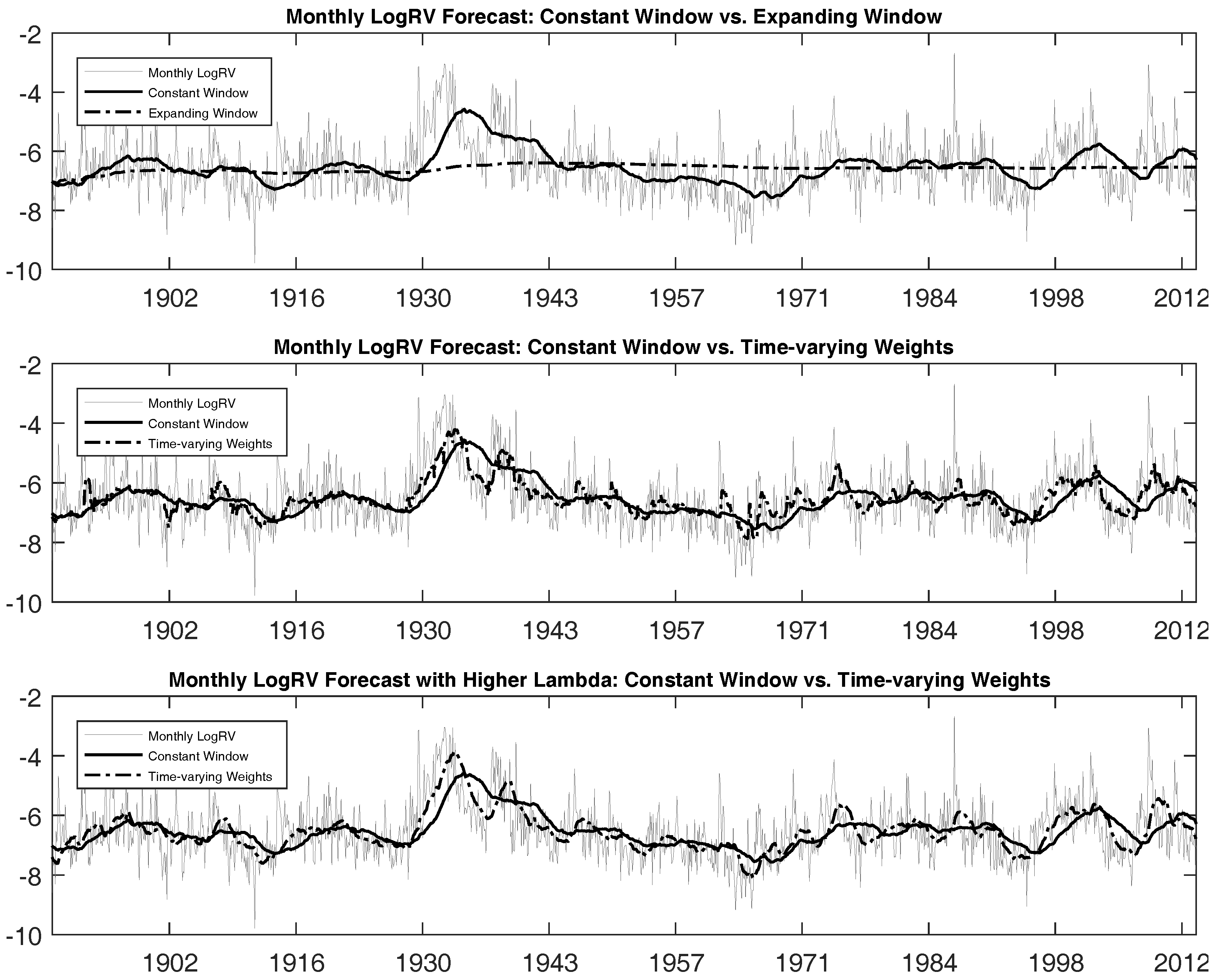
Figure 3 graphically illustrates these results by plotting the target logRV against model predictions. We see that using the entire data sample weighted equally as in the $M_1$ model generates forecasts that are too smooth, being unable to capture the frequently-occurring model changes of the logRV process. In contrast, taking the recent five years of observations allows forecasts to respond to the model changes in a better fashion. However, this $M_{t-60}$ model still lacks the ability to react fast enough.

Now, we turn our attention to the our model $M_{*}$ that uses data histories associated with submodels each period. Improvement in the forecasting performance is quite noticeable with respect to both the bias and efficiency metrics. The $R^2$, that is the proportion of variability in out-of-sample RV explained by forecasts using the $M_{*}$ model, increases to 33.21%, which is more than double that of the $M_{t-60}$ model, and the forecasts are much less biased than those for the other two models as indicated by the intercept and slope coefficients.

Figure 3 illustrates these differences graphically. We see that the model $M_{*}$ is able to react faster to capture possible model change. Note again that all three models we compare are the same model in the statistical sense. They only differ in the data sample we use to estimate the parameters; thus, the difference in the performance should solely come from the difference in data samples used to estimate the parameters and generate the forecasts. Our results, even for the first moment of the monthly realized variance forecasts, illustrate the improvements originating from being able to select time-varying weights of different data histories at each point in time. That is, choosing a fixed-length moving window generates additional bias and forecasts that track our target less efficiently. Overall, this result confirms the importance of using the time-varying weights when making forecasts. We will discuss this in more detail in the next subsection.

In the bottom panel of Table 2, we report the same analyses performed for forecasts of daily logRV from April 2007–February 2015 for three futures. The daily futures RV were constructed from 15-min intraday futures prices as discussed in Section 2 above. For all three SP, GC and CL futures, the model $M_1$ performs poorly as before, while the model $M_{t-60}$ does a much better job. The model $M_{*}$ still remains dominant, particularly providing much less biased forecasts. However, a less dramatic increase in $R^2$ is observed when compared to the model $M_{t-60}$, perhaps indicating that 60 days is close to the best fixed window-length to use for daily realized variance data. It is not too surprising since 60 days has been found to be a good ad hoc number to use by many practitioners. Figures similar to Figure 3 for daily forecasts of three Futures’ logRV exhibit similar findings and are omitted for brevity. More or less, we see the same pattern as for monthly data that the model $M_{*}$ is the best at reacting to model changes in the underlying data.

Next, we perform the same analyses of the Fisher transformed daily realized correlations for the three futures.

Table 3. Forecast regression results for FisRCorr.

	Expanding Window (${\mathit{M}}_{\mathbf{1}}$)	Constant Window (${\mathit{M}}_{\mathit{t}\mathbf{-}\mathbf{60}}$)	Time-Varying Weights (${\mathit{M}}_{\mathbf{*}}$)	Time-Varying Weights (Higher $\mathit{\lambda }$ Prior)
FisRCorr (SP, GC)
Intercept	0.0865	0.0274	−0.0125	−0.0125
	(2.50) **	(2.77) ***	(−1.37)	(−1.38)
Slope	0.4787	0.8247	1.0121	1.0169
	(−3.06) ***	(−5.53) ***	(0.41)	(0.58)
R2	0.40%	25.83%	38.15%	38.50%
FisRCorr (SP, CL)
Intercept	0.1726	0.0414	−0.0076	−0.0146
	(8.26) ***	(3.63) ***	(−0.67)	(−1.30)
Slope	0.6240	0.8844	1.0006	1.0180
	(−5.26) ***	(−4.28) ***	(0.02)	(0.68)
R2	3.77%	35.49%	42.26%	43.55%
FisRCorr (GC, CL)
Intercept	−0.5591	0.0585	−0.0118	−0.0168
	(−5.98) ***	(4.03) ***	(−0.85)	(−1.21)
Slope	2.2142	0.8092	0.9963	1.0215
	(5.26) ***	(−5.17) ***	(−0.11)	(0.61)
R2	4.51%	19.79%	29.21%	30.16%

Notes: Mincer–Zarnowitz regressions of daily realized FisRCorr on forecasts from each model are reported. We use symbols SP, GC and CL to denote S&P500 index, gold and light crude oil futures, respectively. t-statistics for the intercept being different than 0 and the slope being different than 1 are reported in parentheses. ***, **, and * indicate statistical significance at the 1%, 5%, and 10% confidence levels, respectively. R² associated with these forecast regressions indicates the proportion of variability in the out-of-sample realized variable that is predicted by the forecasts.

reports results using the same period of data from April 2007–February 2015 as for the realized variances. Again, the same broad conclusions can be drawn from the realized correlations forecasts. However, improvements in both the bias and the $R^2$ associated with the $M_{*}$ model are more pronounced. In particular, the estimated intercept and slope coefficients are such that forecasts are strikingly close to being unbiased. In addition, the $M_{*}$ model forecasts provide a much better fit in general compared to those for the log of realized variance. It is likely the case that the realized correlations exhibit more variation in the length between the occurrence of model changes. In that case, our model using the time-varying weights is better suited for capturing the realized correlation than the realized variance.

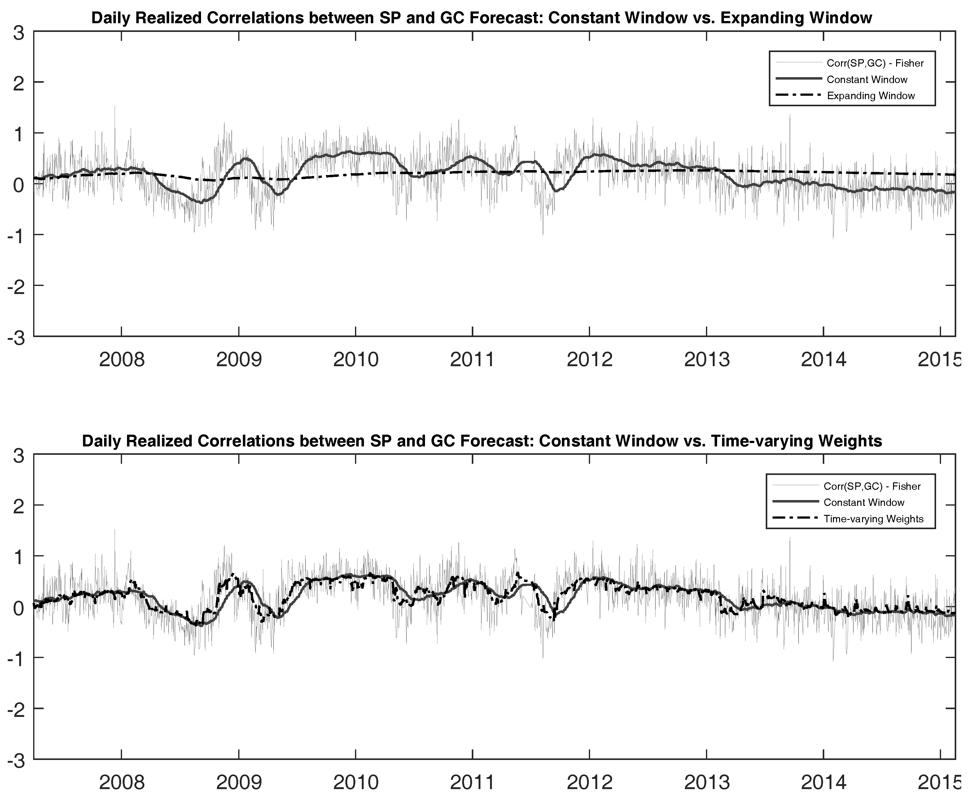
Figure 4 again illustrates the differences between the forecasted values and realized values for correlation between SP and GC futures. The other two cases are omitted for brevity where the same conclusions hold in all cases.

So far, we have been focusing on assessing each model’s ability to forecast the first moment of the underlying process. We now turn our attention to the statistical measure that can assess higher moments, as well, that is the distributions of log(RV)and FisRCorr. Given the normality assumption of the underlying process, the marginal predictive likelihood at each point of time only requires the forecasts of mean and variance of $x_t$. For the case of model $M_{*}$, we compute the forecasts of mean and variance using Equation (A.9), while the sample mean and sample variance of the corresponding data history are used for the benchmark models. Then, the sum of log marginal predictive likelihood is computed by the expression below.

$$\begin{array}{c}\hfill \log (\mathrm{ML})=\sum _{t}log(p(x_t|{\Omega }_{t-1}))\end{array}$$

(23)

Table 4. Log-likelihoods for alternative forecast models.

	Expanding Window (${\mathit{M}}_{\mathbf{1}}$)	Constant Window (${\mathit{M}}_{\mathit{t}\mathbf{-}\mathbf{60}}$)	Time-Varying Weights (${\mathit{M}}_{\mathbf{*}}$)	Time-Varying Weights (Higher $\mathit{\lambda }$ Prior)
Panel A: Monthly Frequency, Sample Period 1885–2013
log(ML): logRV (S&P)	−2043.01	−1929.67	−1742.83	−1714.76
Panel B: Daily Frequency, Sample Period April 2007–February 2015
log(ML): FisRCorr (SP, GC)	−1023.83	−703.28	−542.52	−514.54
log(ML): FisRCorr (SP, CL)	−892.03	−411.52	−345.85	−311.43
log(ML): FisRCorr (GC, CL)	−776.67	−528.84	−418.49	−400.80

Notes: This table reports the sum of the log-likelihoods over the sample periods (log(ML)) for the monthly and daily forecasts. We use Equation (23) to compute log(ML). The top panel reports the log(ML) for monthly logRV of the S&P index. The bottom panel reports log(ML) for daily FisRCorr between three futures contracts.

summarizes these results. Cases with higher prior values on $\lambda$ are again included to make sure our approach is robust to the initial choice of $\lambda$. The results again heavily favour the model $M_{*}$ over the two benchmark models. A dramatic increase in the log-likelihood is observed for all the datasets. The results here are not directly comparable to the MZ regression results discussed above, but they indicate that $M_{*}$ model has superior forecasts of the distributions of realized variance and correlation relative to the benchmark models. Using a Bayes factor criterion for comparison of the log(ML) across models indicates very strong or decisive evidence in favour of the $M_{*}$ model.

Overall, all of the above statistical tests heavily support the model $M_{*}$ over the other two models. Again, the differences are purely coming from the fact that each model uses different data histories, thus highlighting the importance of having a flexible framework to capture model changes in the underlying data.

4.2. Submodel Probability Distributions

The submodel probability distribution at each point in time indicates how much weight the model $M_{*}$ allocates to each of the submodels available at that time; that is, for all of the submodels from the start of the sample to the current time. Although all available submodels are considered, the peak of the submodel distribution at each point of time identifies the submodel that receives the most weight from the perspective of maximizing the $M_{*}$ model’s predictive content at that time. Optimal submodel weights are estimated for each period, and new submodels are added as we move through time. The top panel of Figure 5 provides a 3D plot of how the submodel probability distribution varies over time for the $M_{*}$ model’s predictive density for monthly logRV from 1885–2013. The y-axis represents the index of each submodel $M_{\tau }$, that is the time $\tau$ that a submodel was introduced; the x-axis represents each time period; and the vertical axis represents the probability associated with submodel $M_{\tau }$ at each time t. If the submodel distribution has a high peak, it means that most of the submodel probability weight is concentrated on that specific submodel, that is very few submodels, perhaps only one, have meaningful contributions to the model $M_{*}$. In contrast, a lower peak and wider spread over the y-axis means that there are many submodels that contribute to the model $M_{*}$ forecasts.

The bottom panel of Figure 5 is a 2D-plot representing the time-varying weight associated with some specific submodels over time. In other words, it is a slice from the plot in the top panel of Figure 5 when we fix the y-axis to be the specific submodel introduced at that time. The solid line represents the submodel probabilities associated with the submodel starting from year 1886. We observe that it has a weight almost equal to one at the beginning, then loses its weight significantly and rather quickly. The other three dotted lines represent the submodels starting from 1926, 1976 and 2006, respectively, from left to right. These submodels get less weight over time, perhaps due to the changes in the fundamentals of the data-generating process. In particular, the submodel starting from 2006 has very little weight, and its contribution disappears almost immediately. This is in line with the fact that the financial crisis of 2008 made the past data almost useless as the realized variance shoots up during the crisis periods. Thus, it again confirms the ability of our model to learn in real time by assigning very little probability weight to submodels that provide no predictive content.

4.3. Time-Varying Window Length

Given the results in the previous section, we now turn to a the deeper analysis of why the model $M_{*}$ performs so well. In order to do so, we introduce the measure that we call time-varying window length ($W^{*}$), designed to suggest a length of data history to be used at each time period. Loosely speaking, we can think that the model $M_{t-60}$ corresponds to the case where $W^{*}$ is equal to 60 in all time periods.

To construct $W^{*}$, recall from Equation (19) that we have the posterior submodel probabilities for each submodel $M_{\tau }$. Since each submodel $M_{\tau }$ corresponds to the model using the data window of length $t+1-\tau$, we can compute the average length of the data window at time t by averaging these by the submodel probabilities. Thus, we define $W^{*}$ at time t as follows:

$$\begin{array}{c}\hfill W_t^{*}=\sum _{\tau =1}^t(t+1-\tau )p(M_{\tau }|{\Omega }_t).\end{array}$$

(24)

For example, consider the following artificial case. Suppose that $t=3$ and the submodel probabilities are calibrated to be $p(M_1|{\Omega }_t)=0.2$, $p(M_2|{\Omega }_t)=0.6$ and $p(M_3|{\Omega }_t)=0.2$. In this case, using the above formula, we have $W_t^{*}=2$. Note that the model $M_{*}$ in this case not only uses the submodel $M_2$, but also uses the submodels $M_1$ and $M_3$ with lower probability weights. However, since the highest weight is placed on the submodel $M_2$, the $W_t^{*}$ measure turns out to be two to represent that the average length of the data history is two at that point in time. Therefore, $W_t^{*}$, at each t, provides a convenient measure of a time-varying window length.

Table 5. Summary statistics for time-varying window length.

Symbol	Mean	Std. Dev.	Skewness	Kurtosis
Panel A: Monthly Frequency, Sample Period 1885–2013
logRV (S&P)	23.60	10.98	0.907	3.797
Panel B: Daily Frequency, Sample Period April 2007–February 2015
FisRCorr (SP, GC)	68.47	54.46	1.489	4.757
FisRCorr (SP, CL)	66.60	36.75	0.741	3.101
FisRCorr (GC, CL)	87.69	55.88	1.176	4.599

Notes: We report the descriptive statistics of time-varying window length for monthly logRV of the S&P index and daily FisRCorr between three futures contracts. Time-varying window length is computed using Equation (24).

summarizes the descriptive statistics of the $W^{*}$ measures over the sample period. We see that the mean $W^{*}$ for monthly logRV is around 24, being much smaller than 60. Meanwhile, the mean $W^{*}$ for daily FisRCorr data are closer to 60 days for the (SP, GC) and (SP, CL) pairs and a bit larger than 60 days for the (GC, CL) pair. This provides an explanation as to the difference in performance for each dataset we observed using MZ regressions. If the mean $W^{*}$ is close to 60, the model $M_{t-60}$ will perform much better relative to the $M_{*}$ model than the case for which the mean $W^{*}$ is far from 60, as in the case of monthly logRV.

Table 6. Characteristics of the underlying data for time-varying window length.

Panel A: Cross-Sectional Characteristics
	W*	Characteristics of Correlation Time-Series
Symbol	Mean	Standard Deviation	AR(1) Coefficient	AR(2) Coefficient
Daily Frequency, Sample Period April 2007–February 2015
FisRCorr (SP, GC)	68.47	0.4069	0.5570	0.5200
FisRCorr (SP, CL)	66.60	0.3792	0.5690	0.5372
FisRCorr (GC, CL)	87.69	0.3589	0.4202	0.3964
Panel B: Time-Series Regression on VIX
Symbol	Intercept	VIX	R2	N
Daily Frequency, Sample Period April 2007–February 2015
FisRCorr(SP,GC)	110.8256	−1.9169	13.25%	1949
	(40.86) ***	(−17.24) ***
FisRCorr(SP,CL)	88.6728	−0.9988	7.90%	1949
	(47.02) ***	(−12.92) ***
FisRCorr(GC,CL)	146.98	−2.6829	24.64%	1949
	(56.66) ***	(−25.23) ***

Notes: In Panel A, we report the characteristics of the underlying data, as well as mean time-varying window length for daily FisRCorr between three futures contracts. The time-varying window length is computed using Equation (24).

$$\begin{array}{c}\hfill W_t^{*}=\sum _{\tau =1}^t(t+1-\tau )p(M_{\tau }|{\Omega }_t)\end{array}$$

In Panel B, we report the linear regression result of regressing the $W^{*}$ time series on VIX. t-statistics are reported in parentheses below coefficient estimates. ***, **, and * indicate statistical significance at the 1%, 5%, and 10% confidence levels, respectively.

$$\begin{array}{c}\hfill W_t^{*}=a+bVI{X}_t+{ϵ}_t\end{array}$$

provides two analyses of the characteristics of the underlying data that influence the mean $W^{*}$. To have a valid comparison, we only present the results for FisRCorr as they have equal sample periods. We first observe that FisRCorr (GC, CL) has the smallest standard deviation of the three series and exhibits the longest length for the mean $W^{*}$ measure. Moreover, the levels of persistence, as measured by the first two autocorrelation coefficients, show that the less persistent time series have a longer mean window length. This is particularly pronounced for FisRCorr (GC, CL).

We next examine potential sources of the time series variability of $W^{*}$. Our forecasting approach was designed to capture probabilistic model change, such as regime switches, varying importance of economic fundamentals, etc., as revealed in the changing data generating process (DGP). We chose CBOE (Chicago Board Options Exchange) Volatility Index, VIX, as an indicator or representative variable to proxy the business conditions or economic regime at each point of time. Larger VIX values are interpreted as bad states, while smaller VIX values are viewed as good states. Panel B of Table 6 reports the results of simple linear regressions to test the relationship between the VIX index and three $W^{*}$ time series of interest. The estimated coefficients associated with the VIX index are all negative and statistically significant, indicating that high VIX periods are associated with low $W^{*}$ values, and vice versa. This finding suggests that our forecasting approach adjusts the length of data history to be used at each point of time (time-variation in the $W^{*}$ data), at least partly in response to changes in the DGP.

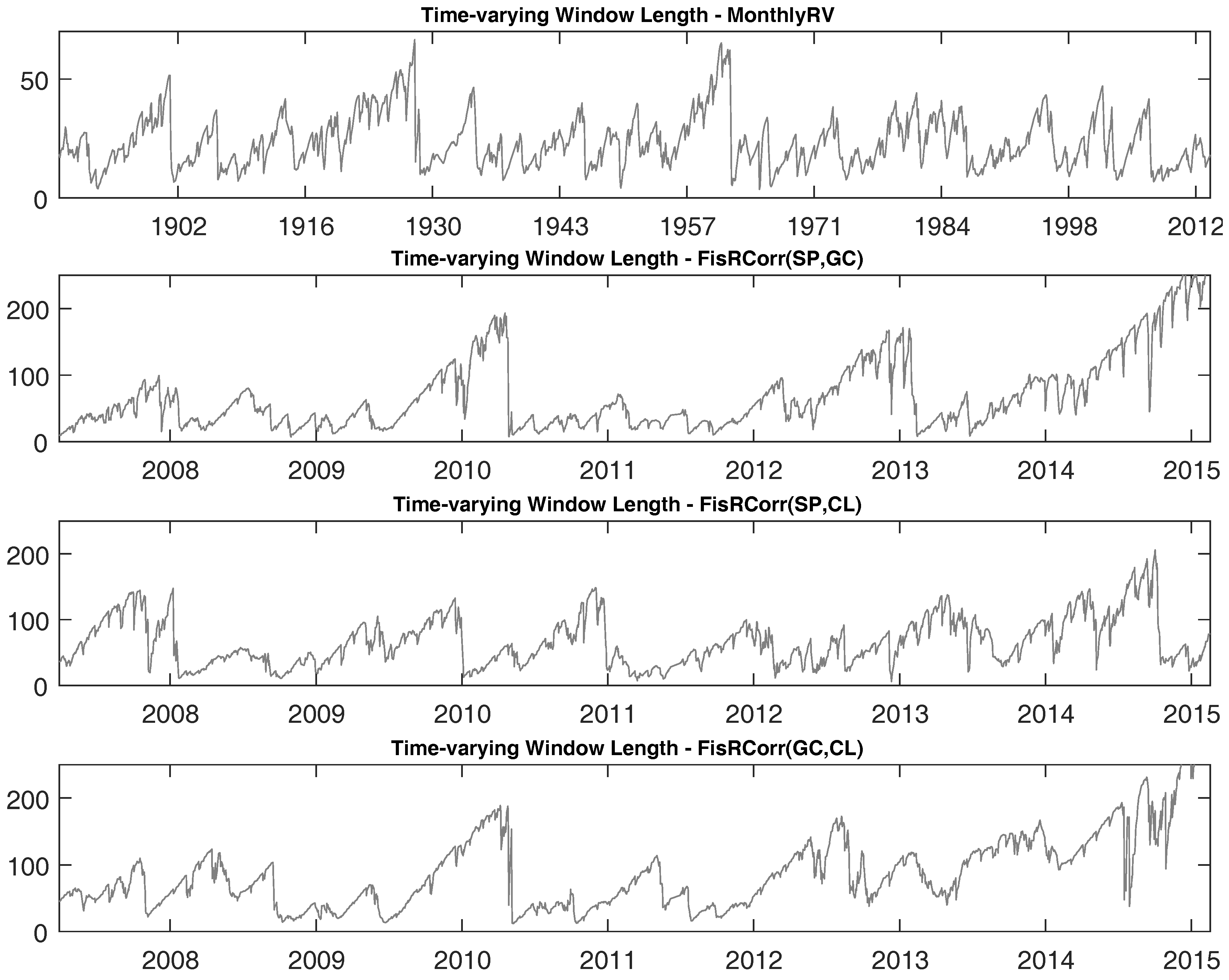
To observe how $W^{*}$ varies over time, we plot the time series of $W^{*}$ in Figure 6. There is significant time variation revealed for the $W^{*}$ time series for all of our realized variance and correlation datasets. For the case of realized correlations, $W^{*}$ can be as small as a single digit and can be as large as almost 250 days, roughly a year, depending on the time period. Our forecasting approach was designed to learn about changes in the DGP and update the submodel probabilities accordingly. When the submodel probabilities change, the time-varying window $W^{*}$ measure will change.

4.4. Time-Varying Window Model

Recall that our optimal data-use model, $M_{*}$, generates forecasts using information from all of the submodels, appropriately weighted by their time-varying submodel probabilities that maximize the forecasting power. That is, $M_{*}$ assigns probability weights to the available submodels (data histories) where each submodel is estimated separately, then the resulting submodel forecast are aggregated by the submodel probability weights (in combination with the estimated model change probability). Thus, that approach uses the entire data history available from $t=1$, but assigns different weights to each data history covered by each submodel.

Alternatively, we can truncate the data history, every period, at the point of most mass for the submodel probability distribution for that period, which we estimate as the time-varying window length ($W^{*}$). Then, we can fix the length of the data window, each period, using this $W^{*}$ measure and compute our forecasts using that data window. In other words, in contrast to $M_{*}$, we switch the order of aggregation in that we aggregate the data histories to the length of the $W^{*}$ window first and then estimate the model and forecast using data corresponding to that window length. Of course, the length of this window will vary over time as $W^{*}$ varies period-by-period. We will write this $W^{*}$ model as $M_{W^{*}}$.

Table 7. Time-varying weights versus time-varying window results.

	Time-Varying Weights (${\mathit{M}}_{*}$)	Time-Varying Window (${\mathit{M}}_{{\mathit{W}}^{*}}$)
Panel A: Monthly Frequency, Sample Period 1885–2013
logRV (S&P)
Intercept	−0.2893	−0.7724
	(−1.25)	(−4.11) ***
Slope	0.9574	0.8835
	(−1.21)	(−4.06) ***
R2	33.21%	39.00%
log(ML )	−1714.76	−1778.72
Panel B: Daily Frequency, Sample Period April 2007–February 2015
FisRCorr (SP, GC)
Intercept	−0.0125	−0.0027
	(−1.37)	(−0.31)
Slope	1.0121	0.9507
	(0.41)	(−1.91) *
R2	38.15%	41.17%
log(ML)	−514.54	−524.53
FisRCorr (SP, CL)
Intercept	−0.0076	0.0056
	(−0.67)	(0.53)
Slope	1.0006	0.9634
	(0.02)	(−1.53)
R2	42.26%	45.38%
log(ML)	−311.43	−298.23
FisRCorr (GC, CL)
Intercept	−0.0118	0.0143
	(−0.85)	(1.11)
Slope	0.9963	0.9263
	(−0.11)	(−2.34) **
R2	29.21%	30.16%
log(ML)	−400.80	−404.22

Notes: Mincer–Zarnowitz regressions of monthly logRV of the S&P index and daily FisRCorr of three futures contracts on forecasts from two time-varying models are reported. t-statistics for the intercept being different than 0 and the slope being different than 1 are reported in parentheses. ***, **, and * indicate statistical significance at the 1%, 5%, and 10% confidence levels, respectively. R² associated with the Mincer–Zarnowitz regressions indicates the proportion of variability in the out-of-sample realized variable that is predicted by the forecasts.

reports comparison between these two time-varying data-use models. Interestingly, we see that $R^2$ of the Mincer–Zarnowitz regression is higher using the $M_{W^{*}}$ model in almost all datasets, but at the same time, as indicated by the intercept and slope coefficients, the forecasts are more biased than the $M_{*}$ forecasts, but still significantly less biased than in the two benchmark models.

The only difference between the forecasts associated with model $M_{W^{*}}$ and the forecasts from the benchmark models, $M_1$ and $M_{t-60}$, is the length of the data window. The fact that the $M_{W^{*}}$ forecasts are better than the benchmark model with respect to both bias and $R^2$ (that is, the proportion of the variation in the target explained by the forecast) confirms that it uses the better length of data window, period-by-period, that drives the superior performance of our approach.

Note that when we compare the log-likelihoods across the two models in Table 7, the time-varying weights model $M_{*}$ forecasts the distributions slightly better than the time-varying window model $M_{W^{*}}$. This is not surprising given that the $M_{*}$ model updates all submodel probabilities period-by-period based on their predictive content and uses those optimal weights to compute out-of-sample forecasts; whereas the $M_{W^{*}}$ model first finds the submodel (data history) that has the most predictive content and then fixes the forecast estimation window at that value for that period.

It is clear from comparing the log-likelihood results reported in Table 7 to those for the benchmark models reported in Columns 2 and 3 of Table 4, as well as from the Mincer–Zarnowitz forecast regression results presented in earlier tables and figures, the forecasts from both the time-varying weights model $M_{*}$ and the time-varying window model $M_{W^{*}}$ are far superior to the conventional benchmark forecasts.

5. Robustness

5.1. Model Comparison with Alternative Metrics

This subsection revisits the model comparisons using alternative metrics. Recall that we have used two metrics, coefficients and $R^2$ from forecast regressions, to compare alternative models. We now compare our models using two additional metrics, mean absolute error (MAE) and sum of squared errors (SSE), both from the same Mincer–Zarnowitz forecast evaluation regressions. Two quantities are defined below in which we use the estimated coefficients $\widehat{a}$ and $\widehat{b}$ discussed in Section 4:

$$\begin{array}{ccc}\hfill {\mathrm{MAE}}_i|M& =& \frac{1}{T}\sum _{t=1}^T|{\log \mathrm{RV}}_{i,t}-\widehat{a}-\widehat{b}{E}_{t-1}[{\log \mathrm{RV}}_{i,t}|{\Omega }_{t-1},M]|\hfill \end{array}$$

(25)

$$\begin{array}{ccc}\hfill \mathrm{average}{\mathrm{SSE}}_i|M& =& \frac{1}{T}\sum _{t=1}^T{({\log \mathrm{RV}}_{i,t}-\widehat{a}-\widehat{b}{E}_{t-1}[{\log \mathrm{RV}}_{i,t}|{\Omega }_{t-1},M])}^2\hfill \end{array}$$

(26)

Table 8. MAE and SSE from forecast regressions.

	Expanding Window (${\mathit{M}}_{\mathbf{1}}$)	Constant Window (${\mathit{M}}_{\mathbf{t}-\mathbf{60}}$)	Time-Varying Weights (${\mathit{M}}_{*}$)	Time-Varying Window (${\mathit{M}}_{{\mathit{W}}^{*}}$)
Panel A: Monthly Frequency, Sample Period 1885–2013
logRV (S&P)
MAE	0.7230	0.6723	0.5986	0.5740
avg. SSE	0.9012	0.7568	0.6027	0.5505
Panel B: Daily Frequency, Sample Period April 2007–February 2015
FisRCorr (SP, GC)
MAE	0.3319	0.2749	0.2500	0.2430
avg. SSE	0.1649	0.1228	0.1024	0.0974
FisRCorr (SP, CL)
MAE	0.2987	0.2366	0.2263	0.2201
avg. SSE	0.1383	0.0927	0.0830	0.0785
FisRCorr (GC, CL)
MAE	0.2784	0.2490	0.2339	0.2314
avg.SSE	0.1229	0.1032	0.0911	0.0892

Notes: Mean absolute error (MAE) and average sum of squared errors (avg. SSE) from Mincer–Zarnowitz regressions for each model are reported.

$$\begin{array}{ccc}\hfill {MAE}_i|M& =& \frac{1}{T}\sum _{t=1}^T|{\log \mathrm{RV}}_{i,t}-\widehat{a}-\widehat{b}{E}_{t-1}[{\log \mathrm{RV}}_{i,t}|{\Omega }_{t-1},M]|\hfill \\ \hfill \mathrm{avg}.{\mathrm{SSE}}_i|M& =& \frac{1}{T}\sum _{t=1}^T{({\log \mathrm{RV}}_{i,t}-\widehat{a}-\widehat{b}{E}_{t-1}[{\log \mathrm{RV}}_{i,t}|{\Omega }_{t-1},M])}^2\hfill \end{array}$$

reports comparisons between our four models, $M_1$, $M_{t-60}$, $M_{*}$ and $M_{W^{*}}$, using these two metrics. Overall, qualitatively, the same result holds for both metrics. As before, $M_{*}$ and $M_{W^{*}}$ outperform the benchmark $M_1$ and $M_{t-60}$ models significantly across all datasets. Interestingly, our time-varying window model $M_{W^{*}}$ outperforms the time-varying weights model $M_{*}$ in all four datasets we consider and for both metrics.

5.2. Long-Horizon Forecasting

So far, our main variable of interest to be forecasted was limited to one-day-ahead realized measures. One might question whether the forecasting power comes from high persistence associated with the time series of the realized measures rather than from superior forecasting models. We therefore check whether our proposed models also have superior forecasting power in the long-horizon, as well. Specifically, we replace the target measure (dependent variable in the Mincer–Zarnowitz forecast regression) with the average realized measures of the next 60 periods from $t+1$–$t+60$. For example, the Mincer–Zarnowitz regression for logRV using the forecasts from model M takes the following form:7

$$\begin{array}{c}\hfill \frac{1}{60}\sum _{j=1}^{60}\log R{V}_{i;t-1+j}=\log R{V}_{i,t\to t+60}=a+b\times E_{t-1}[\log R{V}_{i;t}|{\Omega }_{t-1},M]+u_t\end{array}$$

Table 9. Forecast regression results for long-horizon .

	Expanding Window (${\mathit{M}}_{\mathbf{1}}$)	Constant Window (${\mathit{M}}_{\mathit{t}-\mathbf{60}}$)	Time-Varying Weights (${\mathit{M}}_{*}$)	Expanding Window (${\mathit{M}}_{\mathbf{1}}$)	Constant Window (${\mathit{M}}_{\mathit{t}-\mathbf{60}}$)	Time-Varying Weights (${\mathit{M}}_{*}$)
	Panel A: Monthly Frequency, Sample Period 1885–2013
	logRV(S&P)
Intercept	−11.7138	−4.4630	−4.2274
	(−2.58) ***	(−4.17) ***	(−5.09) ***
Slope	-0.7887	0.3134	0.3506
	(−2.60) ***	(−4.23) ***	(−5.38) ***
R2	3.30%	9.99%	18.57%
	Panel B: Daily Frequency, Sample Period April 2007–February 2015
	logRV (SP)			FisRCorr (SP, GC)
Intercept	−7.9923	−3.1354	−3.7217	0.2784	0.0909	0.0784
	(−2.00) **	(−2.68) ***	(−3.88) ***	(1.57)	(1.50)	(1.63)
Slope	0.2309	0.6957	0.6409	−0.4652	0.4907	0.5364
	(−1.95) *	(−2.86) ***	(−4.08) ***	(−1.80) *	(−2.90) ***	(−3.32) ***
R2	0.78%	49.02%	52.65%	1.00%	22.78%	33.15%
	logRV (GC)			FisRCorr (SP, CL)
Intercept	−2.0881	−3.1775	−3.4293	0.2426	0.1218	0.1060
	(−0.28)	(−2.22) **	(−3.05) ***	(1.65) *	(1.46)	(1.63)
Slope	0.8229	0.7010	0.6787	0.3888	0.6604	0.6872
	(−0.25)	(−2.26) **	(−3.07) ***	(−1.32)	(−1.95) *	(−2.30) **
R2	4.53%	48.90%	53.14%	3.32%	45.20%	52.74%
	logRV (CL)			FisRCorr (GC, CL)
Intercept	5.0959	−1.7683	−1.5729	0.0456	0.1597	0.1490
	(0.84)	(−1.18)	(−1.19)	(0.09)	(2.27) **	(2.58) ***
Slope	1.6283	0.8072	0.8299	0.7226	0.5127	0.5356
	(0.91)	(−1.22)	(−1.22)	(−0.22)	(−2.84) **	(−3.32) ***
R2	18.13%	64.29%	67.59%	1.44%	24.94%	32.40%

Notes: Mincer–Zarnowitz regressions from each model are reported where the forecast variable of interest is the long-horizon (60 periods) average. t-statistics for the intercept being different than 0 and the slope being different than 1 are reported in parentheses. ***, **, and * indicate statistical significance at the 1%, 5%, and 10% confidence levels, respectively. We use the adjustment of Hansen and Hodrick (1980) for standard errors to compute t-statistics robust to overlapping data. R² associated with these forecast regressions indicates the proportion of variability in the out-of-sample realized variable that is predicted by the forecasts.

summarizes the results from the long-horizon Mincer–Zarnowitz regressions. The overall results are largely consistent with Table 2 and Table 3. The time-varying weights model always exhibits the highest $R^2$ compared to the two benchmark models, an expanding window weighting historical data equally and a constant fixed-length window, in all realized measures we consider. The improvement is not as large as the one-day-ahead forecast, but still relatively large for measures such as monthly logRV (S&P) and FisRCorr (SP, GC). Note that the time-varying weights model still outperforms the constant window model, which conditions on information from the past 60 periods, which is equal to the forecasting horizon. The reason behind the superior performance of the time-varying weights model is that it provides a forecast of the unconditional mean of the underlying data-generating process; thus, it should perform well in forecasting a long-horizon, which proxies the unconditional mean. We hence conclude that the time-varying weights approach is robust to long-horizon forecasting, outperforming using all of the historical data weighted equally or using a fixed-length moving window.

5.3. Alternative Forecasting Methods

Note that our approach is not dependent on a particular choice of statistical model as we do not impose any restrictions on the forecasting method itself. Rather, our approach addresses the issue of how many historical data to use and how to weight those data. All of the results we have shown so far have compared our time-varying weights and time-varying window approaches to two benchmark methods of computing a forecast of the sample average of the realized measures. A natural question that arises is whether more sophisticated forecasting models of realized measures can alter our findings.

We now show the robustness of our preferred time-varying window model, ($M_{W^{*}}$), for two alternative statistical approaches: exponentially-weighted moving-average (ExpWMA) and AR(1) models. Specifically, we re-estimate the time-varying window model, as well as our two benchmark data usage models, expanding window and constant window, for the $ExpWMA$ and AR(1) forecasting models.

Table 10. Forecast regression results for the exponentially-weighted moving-average (ExpWMA) method.

	Expanding Window (${\mathit{M}}_{\mathbf{1}}$)	Constant Window (${\mathit{M}}_{\mathit{t}-\mathbf{60}}$)	Time-Varying Window (${\mathit{M}}_{{\mathit{W}}^{*}}$)	Expanding Window (${\mathit{M}}_{\mathbf{1}}$)	Constant Window (${\mathit{M}}_{\mathit{t}-\mathbf{60}}$)	Time-Varying Window (${\mathit{M}}_{{\mathit{W}}^{*}}$)
	Panel A: Monthly Frequency, Sample Period 1885–2013
	logRV(S&P)
Intercept	−0.3687	−0.8555	−0.7179
	(−1.31)	(−3.46) ***	(−3.92) **
Slope	0.9414	0.8677	0.8915
	(−1.37)	(−3.51) ***	(−3.88) ***
R2	24.62%	26.33%	40.65%
	Panel B: Daily Frequency, Sample Period April 2007–February 2015
	logRV (SP)			FisRCorr (SP, GC)
Intercept	−0.2745	−0.3506	−0.8070	0.0044	0.0068	0.0057
	(−1.26)	(−1.62)	(−4.23) ***	(0.50)	(0.78)	(0.69)
Slope	0.9734	0.9660	0.9234	0.9616	0.9495	0.9417
	(−1.27)	(−1.63)	(−4.17) ***	(−1.41)	(−1.89) *	(−2.38) **
R2	51.98%	52.09%	55.97%	39.16%	39.34%	43.28%
	logRV (GC)			FisRCorr (SP, CL)
Intercept	−0.5998	−0.6796	−0.8829	0.0137	0.0159	0.0119
	(−1.81) *	(−2.07) **	(−2.82) ***	(1.31)	(1.53)	(1.18)
Slope	0.9440	0.9364	0.9183	0.9629	0.9559	0.9554
	(−1.79) *	(−2.06) **	(−2.77) ***	(−1.52)	(−1.83) *	(−1.95) *
R2	31.49%	31.55%	32.87%	44.41%	44.55%	47.11%
	logRV (CL)			FisRCorr (GC, CL)
Intercept	−0.1723	−0.2160	−0.3162	0.0157	0.0200	0.0230
	(−0.88)	(−1.12)	(−1.68) *	(1.22)	(1.58)	(1.91) *
Slope	0.9804	0.9757	0.9663	0.9436	0.9314	0.9182
	(−0.93)	(−1.16)	(−1.66) *	(−1.74) *	(−2.15) **	(−2.77) ***
R2	52.09%	52.22%	53.19%	30.44%	30.53%	33.11%

Notes: Mincer–Zarnowitz regressions from each model are reported where the forecasts are generated using the exponentially-weighted moving-average method. For monthly frequency, a smoothing parameter of 0.97 was used, and for daily data, a smoothing parameter of 0.94 was used. t-statistics for the intercept being different than 0 and the slope being different than 1 are reported in parentheses. ***, **, and * indicate statistical significance at the 1%, 5%, and 10% confidence levels, respectively. R² associated with these forecast regressions indicates the proportion of variability in the out-of-sample realized variable that is predicted by the forecasts.

reports results for an exponentially-weighted moving average model with a smoothing parameter of 0.97 for monthly data and 0.94 for daily data, following RiskMetrics . Since exponential weighting of the historical data already captures a portion of the forecasting power, the improvement in the $R^2$ using a time-varying window model is not as significant as it was in the results summarized in our previous sections. Nevertheless, we still see marginal improvements in $R^2$ associated with the forecasts for all the realized measures, with some notable improvements in the monthly logRV (S&P) forecast.

Next, in

Table 11. Forecast regression results for the AR(1) method.

	Expanding Window (${\mathit{M}}_{\mathbf{1}}$)	Constant Window (${\mathit{M}}_{\mathit{t}-\mathbf{60}}$)	Time-Varying Window (${\mathit{M}}_{{\mathit{W}}^{*}}$)	Expanding Window (${\mathit{M}}_{\mathbf{1}}$)	Constant Window (${\mathit{M}}_{\mathit{t}-\mathbf{60}}$)	Time-Varying Window (${\mathit{M}}_{{\mathit{W}}^{*}}$)
	Panel A: Monthly Frequency, Sample Period 1885–2013
	logRV(S&P)
Intercept	0.1959	−0.3810	−1.1933
	(0.96)	(−2.12) **	(−7.37) ***
Slope	1.0257	0.9424	0.8183
	(0.83)	(−2.10) **	(−7.36) ***
R2	42.72%	44.33%	42.58%
	Panel B: Daily Frequency, Sample Period April 2007–February 2015
	logRV(SP)			FisRCorr(SP,GC)
Intercept	−0.4016	−0.6282	−1.1191	−0.0107	0.0054	0.0030
	(−1.86) *	(−3.28) ***	(−6.28) ***	(−1.07)	(0.63)	(0.36)
Slope	0.9662	0.9406	0.8932	1.0062	0.9354	0.9277
	(−1.61)	(−3.22) ***	(−6.22) ***	(0.18)	(−2.46) **	(−3.00) ***
R2	51.69%	56.63%	57.69%	31.08%	39.57%	42.99%
	logRV(GC)			FisRCorr(SP,CL)
Intercept	−0.3448	−1.2086	−1.5986	0.0426	0.0098	0.0210
	(−0.76)	(−3.70) ***	(−5.29) ***	(3.55) ***	(0.94)	(2.08) **
Slope	0.9801	0.8874	0.8516	0.9403	0.9572	0.9235
	(−0.46)	(−3.66) ***	(−5.21) ***	(−1.95) *	(−1.78) *	(−3.36) ***
R2	20.67%	29.56%	31.06%	32.56%	44.82%	45.81%
	logRV(CL)			FisRCorr(GC,CL)
Intercept	1.1764	−0.2740	−0.2449	−0.0685	0.0290	0.0253
	(3.99) ***	(−1.33)	(−1.23)	(−3.38) ***	(2.20) **	(2.04) **
Slope	1.1495	0.9690	0.9738	1.0744	0.8924	0.8949
	(4.59) ***	(−1.40)	(−1.22)	(1.47)	(−3.28) ***	(−3.47) ***
R2	38.48%	48.93%	50.66%	18.84%	27.49%	31.00%

Notes: Mincer–Zarnowitz regressions from each model are reported where the forecasts are generated from an AR(1) method. t-statistics for the intercept being different than 0 and the slope being different than 1 are reported in parentheses. ***, **, and * indicate statistical significance at the 1%, 5%, and 10% confidence levels, respectively. R² associated with these forecast regressions indicates the proportion of variability in the out-of-sample realized variable that is predicted by the forecasts.

, we report results using an AR(1) forecasting model. Those results are largely consistent with Table 10. Interestingly, the constant window model now performs the best in forecasting the monthly logRV(S&P) . However, for all other realized measures, the time-varying window model still performs the best.

Note that the time-varying window model, $M_{W^{*}}$, applied for these two tables was handicapped in the following sense. The time-varying window measure, $W^{*}$, was constructed from the time-varying weights model that maximizes the forecasting power for an equally-weighted average forecast, In other words, the superior performance of the time-varying window model using $ExpWMA$ or AR(1) forecasting methods is not obvious. If those alternative statistical forecasting methods were integrated into the time-varying weights estimation, the $M_{W^{*}}$ approach would be expected to perform even better than the simple robustness results presented in this section. Therefore, we conclude that our method of combining data histories through time-varying weights is robust to the alternative forecasting methods.

6. Concluding Comments

In complex environments with material uncertainty about the future, almost all strategic decisions depend on good forecasts. Forecasting out-of-sample is fraught with potential biases and inefficiencies arising from model uncertainty. Sources of the latter include uncertainty about changing fundamentals and associated parameters (model instability), structural breaks and nonlinearities due, for example, to regime switching.

In this paper, we focus on forecasting correlations of stock returns with commodities. Correlations between stock returns and commodities are particularly important since they measure how much diversification benefit can be achieved by investing across different asset classes. The time series of variances and correlations between stocks and commodities exhibit frequent shifts. This feature makes forecasting challenging. Using a longer data sample does not necessarily lead to better forecasts and can possibly introduce additional bias. On the other hand, using a fixed-length moving window requires some method of selecting the best window length. Since forecasts are often sensitive to the data sample used to derive the forecast, an approach that weights historical data according to their predictive content at each point in time should provide superior real-time forecasts in the presence of uncertainty about changes in the data generating process.

We evaluate two alternative data usage models, which we compare to standard benchmarks. Our first alternative, a ‘time-varying weights’ model, uses all of the available data and estimates weights for data histories (submodels) according to their their out-of-sample predictive content. Bayesian model average forecasts for each period combine an estimated model change probability with a probability-weighted average of submodel forecasts, integrating out submodel uncertainty. Our second alternative, a ‘time-varying window’ model, builds on the ‘time-varying weights’ model by truncating the data history, every period, at the point of most mass for the submodel probability distribution. We redo our forecasts using this time-varying window length. Our empirical analyses reveal that these two alternative data usage models provide superior forecasts to several benchmark models for forecasting correlations.

We compare our time-varying weights and time-varying window models of data usage to standard benchmarks. Our first benchmark is the sample average of realized variances and realized correlations based on an expanding window as new data arrive. Our second benchmark, motivated by industry practice, is the moving average associated with a fixed-length moving window. Further, since our method is not dependent on any particular forecasting model, but rather evaluates alternative data usage models, we provide several robustness checks for the forecasting efficacy of the time-varying weights and time-varying window approaches. These include long-horizon forecasts, as well as exponentially-weighted moving average and AR(1) forecasting models.

References

1. Andersen, Torben G., Tim Bollerslev, Peter Christoffersen, and Francis X. Diebold. 2007. Practical Volatility and Correlation Modeling for Financial Market Risk Management. In The NBER Volume on Risks of Financial Institutions. Chicago: University of Chicago Press. [Google Scholar]
2. Andersen, Torben G., Tim Bollerslev, Francis X. Diebold, and Paul Labys. 2001. The Distribution of Realized Exchange Rate Volatility. Journal of the American Statistical Association 96: 42–55. [Google Scholar] [CrossRef]
3. Andersen, Torben G., Tim Bollerslev, Francis X. Diebold, and Paul Labys. 2003. Modeling and Forecasting Realized Volatility. Econometrica 71: 579–625. [Google Scholar] [CrossRef]
4. Andersen, Torben G., Tim Bollerslev, and Nour Meddahi. 2005. Correcting the Errors: On Volatility Forecast Evaluation Using High-Frequency Data and Realized Volatilities. Econometrica 73: 279–96. [Google Scholar] [CrossRef]
5. Andreou, Elena, and Eric Ghysels. 2002. Detecting Multiple Breaks in Financial Market Volatility Dynamics. Journal of Applied Econometrics 17: 579–600. [Google Scholar] [CrossRef]
6. Aramov, Doron. 2002. Stock Return Predictability and Model Uncertainty. Journal of Financial Economics 64: 423–58. [Google Scholar] [CrossRef]
7. Bandi, Federico M., Jeffrey R. Russell, and Yinghua Zhu. 2008. Using High-Frequency Data in Dynamic Portfolio Choice. Econometric Reviews 27: 163–98. [Google Scholar] [CrossRef]
8. Barndorff-Nielsen, Ole E., and Neil Shephard. 2002. Econometric analysis of realized volatility and its use in estimating stochastic volatility models. Journal of Royal Statistical Society B 64: 253–80. [Google Scholar] [CrossRef]
9. Büyükashin, Bahattin, Michael S. Haigh, and Michel A. Robe. 2010. Commodities and Equities: A "Market of One"? Journal of Alternative Investments 12: 76–95. [Google Scholar] [CrossRef]
10. Chib, Siddhartha. 2001. Markov Chain Monte Carlo Methods: Computation and Inference. In Handbook of Econometrics. Edited by James J. Heckman and Edward E. Leamer. Amsterdam: Elesvier Science. [Google Scholar]
11. Christoffersen, Peter, Bruno Feunou, Kris Jacobs, and Nour Meddahi. 2014. The Economic Value of Realized Volatility: Using High-Frequency Returns for Option Valuation. Journal of Financial and Quantitative Analysis 49: 663–97. [Google Scholar] [CrossRef]
12. Christoffersen, Peter, Asger Lunde, and Kasper Olesen. 2017. Factor Structure in Commodity Futures Return and Volatility. Journal of Financial and Quantitative Analysis. Forthcoming. [Google Scholar] [CrossRef]
13. Corsi, Fulvio. 2009. A Simple Approximate Long-Memory Model of Realized Volatility. Journal of Financial Econometrics 7: 174–96. [Google Scholar] [CrossRef]
14. Corsi, Fulvio, Nicola Fusari, and Davide La Vecchia. 2013. Realizing smiles: Options pricing with realized volatility. Journal of Financial Economics 107: 284–304. [Google Scholar] [CrossRef]
15. Cremers, K. J. Martijn. 2002. Stock Return Predictability: A Bayesian Model Selection Perspective. Review of Financial Studies 15: 1223–49. [Google Scholar] [CrossRef]
16. Diris, Bart F. 2014. Model Uncertainty for Long-Term Investors. Working paper. Rotterdam, The Netherlands: Department of Econometrics, Erasmus University Rotterdam. [Google Scholar]
17. Fleming, Jeff, Chris Kirby, and Barbara Ostdiek. 2003. The economic value of volatility timing using "realized" volatility". Journal of Financial Economics 67: 473–509. [Google Scholar] [CrossRef]
18. Geweke, John. 1997. Using Simulation Methods for Bayesian Econometric Models: Inference, Development, and Communication. Econometric Reviews 18: 1–73. [Google Scholar] [CrossRef]
19. Hansen, Lars Peter, and Robert J. Hodrick. 1980. Forward Exchange Rates as Optimal Predictors of Future Spot Rates: An Econometric Analysis. Journal of Political Economy 88: 829–53. [Google Scholar] [CrossRef]
20. Hansen, Peter R., and Asger Lunde. 2006. Realized Variance and Market Microstructure Noise. Journal of Business & Economic Statistics 24: 127–61. [Google Scholar]
21. Härdle, Wolfgang K., Nikolaus Hautsch, and Andrija Mihoci. 2014. Local Adaptive Multiplicative Error Models for High-Frequency Forecasts. Journal of Applied Econometrics 30: 529–50. [Google Scholar] [CrossRef]
22. Johannes, Michael, and Nicholas Polson. 2005. MCMC Methods for Financial Econometrics. In Handbook of Econometrics. Amsterdam: Elesvier. [Google Scholar]
23. Kim, Chang-Jin, James C. Morley, and Charles R. Nelson. 2005. The Structural Break in the Equity Premium. Journal of Business & Economic Statistics 23: 181–91. [Google Scholar]
24. Lettau, Martin, and Stijn van Nieuwerburgh. 2008. Reconciling the Return Predictability Evidence. Review of Financial Studies 21: 1607–52. [Google Scholar] [CrossRef]
25. Liu, Chun, and John M. Maheu. 2008. Are There Structural Breaks in Realized Volatility? Journal of Financial Econometrics 6: 326–60. [Google Scholar] [CrossRef]
26. Liu, Chun, and John M. Maheu. 2009. Forecasting Realized Volatility: A Bayesian Model Averaging Approach. Journal of Applied Econometrics 24: 709–33. [Google Scholar] [CrossRef]
27. Maheu, John M., and Stephen Gordon. 2008. Learning, Forecasting and Structural Breaks. Journal of Applied Econometrics 23: 553–83. [Google Scholar] [CrossRef]
28. Maheu, John M., and Thomas H. McCurdy. 2002. Nonlinear Features of Realized FX Volatility. Review of Economics and Statistics 84: 668–81. [Google Scholar] [CrossRef]
29. Maheu, John M., and Thomas H. McCurdy. 2009. How Useful are Historical Data for Forecasting the Long-Run Equity Return Distribution? Journal of Business & Economic Statistics 27: 95–112. [Google Scholar]
30. Martnes, Martin, Dick Van Dijk, and MichielDe Pooter. 2004. Modeling and Forecasting S&P500 Volatility: Long Memory, Structural Breaks and Nonlinearlity. Tinbergen Institute Discussion Paper, 2004-067/4. Rotterdam, The Netherlands: Faculty of Economics, Erasmus Universiteit Rotterdam. [Google Scholar]
31. Mincer, Jacob, and Victor Zarnowitz. 1969. The Evaluation of Economic Forecasts. In Economic Forecasts and Expectations: Analysis of Forecasting Behavior and Performance. Cambridge: National Bureau of Economic Research, Inc., pp. 3–46. [Google Scholar]
32. Pastor, L’luboš, and Robert F. Stambaugh. 2001. The Equity Premium and Structural Breaks. Journal of Finance 56: 1207–39. [Google Scholar] [CrossRef]
33. Pastor, L’luboš, and Robert F. Stambaugh. 2012. Are Stocks Really Less Volatile in the Long Run? Journal of Finance 67: 431–78. [Google Scholar] [CrossRef]
34. Paye, Bradley S., and Allan Timmermann. 2006. Instability of Return Prediction Models. Journal of Empirical Finance 13: 274–315. [Google Scholar] [CrossRef]
35. Pesaran, M. Hashem, and Andreas Pick. 2011. Forecast Combination Across Estimation Windows. Journal of Business & Economic Statistics 29: 307–18. [Google Scholar]
36. Pesaran, M. Hashem, and Allan Timmermann. 2002. Market Timing and Return Prediction under Model Uncertainty. Journal of Empirical Finance 9: 495–510. [Google Scholar] [CrossRef]
37. Pesaran, M. Hashem, and Allan Timmermann. 2007. Selection of Estimation Window in the Presence of Breaks. Journal of Econometrics 137: 134–61. [Google Scholar] [CrossRef]
38. Rapach, David E., and Mark E. Wohar. 2006. Structural Breaks and Predictive Regression Models of Aggregate U.S. Stock Returns. Journal of Financial Econometrics 4: 238–74. [Google Scholar] [CrossRef]
39. Robert, Christian P., and George Casella. 1999. Monte Carlo Statistical Methods. New York: Springer. [Google Scholar]
40. Schwert, G. William. 1990. Indexes of U.S. Stock Prices from 1802 to 1987. Journal of Business 63: 399–426. [Google Scholar] [CrossRef]
41. Silvennoinen, Annastiina, and Susan Thorp. 2010. Financialization, Crisis and Commodity Correlations Dynamics. Working paper. Sydney, Australia: Quantitative Finance Research Centre, University of Technology. [Google Scholar]
42. Tang, Ke, and Wei Xiong. 2012. Index Investment and Financialization of Commodities. Financial Analyst Journal 68: 54–74. [Google Scholar] [CrossRef]
43. Welch, Ivo, and Amit Goyal. 2008. A Comprehensive Look at the Empirical Performance of Equity Premium Prediction. Review of Financial Studies 21: 1455–508. [Google Scholar] [CrossRef]
1.
2.
3.
4.
5.
See: Andreou and Ghysels (2002) in volatility; Liu and Maheu (2008) in realized volatility; Maheu and Gordon (2008) in macroeconomic variables; and Maheu and McCurdy (2009) in market return distributions.
6.
The COMEX gold futures (GC) intra-day prices are missing for June 2011 in the raw data. We have thus disregarded this period in the empirical analysis of the paper.
7.
Recall that, under the null of their construction, the realized measures are time-additive.
Figure 1. Daily realized correlations for three futures contracts, April 2007–February 2015. Plots are the daily realized correlation measures for three futures contracts labelled as SP, GC and CL. These daily series are computed using a 15-min grid of changes in log futures prices from TickData beginning 2 April 2007 and ending 17 February 2015.
Econometrics 05 00054 g001
Figure 2. QQ-plot of FisRCorr (Fisher-transformed Realized Correlation), April 2007–February 2015. QQ-plots of Fisher transformed daily realized correlation measures for three futures contracts labelled as SP, GC and CL. These daily series are computed using a 15-min grid of changes in log futures prices from TickData beginning 2 April 2007 and ending 17 February 2015.
Econometrics 05 00054 g002
Figure 3. Monthly S&P logRV Forecasts, 1885–2013. In each plot, the forecasts for monthly logRV from two alternative models are compared to realized logRV for the period 1885–2013. The top plot compares how well the equally-weighted expanding-window forecasts track the one-month-ahead realized logRV as compared to the forecasts from the equally-weighted moving-average model, which uses the past five years of observations. The middle plot compares the M * model’s (time-varying weights) forecasts to the one-month-ahead realized logRV. The bottom plot is the same as the middle plot, except that we use a higher prior for lambda, the probability of model change.
Econometrics 05 00054 g003
Figure 4. Daily FisRCorr (SP, GC) forecasts, April 2007–February 2015. In each plot, the forecasts for daily FisRCorr (SP, GC) from two alternative models are compared to realized FisRCorr (SP, GC) for the period 2 April 2007–17 February 2015. The top plot compares how well the equally-weighted expanding-window forecasts track the one-day-ahead realized FisRCorr (SP, GC) as compared to the forecasts from the equally-weighted moving-average model, which uses the past 60 days of observations. The bottom plot compares the M * model’s (time-varying weights) forecasts to the one-day-ahead realized FisRCorr (SP, GC).
Econometrics 05 00054 g004
Figure 5. Submodel probabilities over time: monthly logRV. The top panel shows the 3D-plot of the submodel probabilities over time with a new submodel being introduced every 12 months. The bottom panel plots are submodel probabilities over time associated with specific submodels for monthly logRV forecasts.
Econometrics 05 00054 g005
Figure 6. Time-varying window length for monthly logRV and daily FisRCorr. The time-varying window length ( W t * ) for monthly logRV and for three series of daily FisRCorr are plotted on the Y-axes; units are in number of months and days, respectively.
Econometrics 05 00054 g006