Twenty-Two Years of Inflation Assessment and Forecasting Experience at the Bulletin of EU & US Inflation and Macroeconomic Analysis

Abstract

The Bulletin of EU & US Inflation and Macroeconomic Analysis (BIAM) is a monthly publication that has been reporting real time analysis and forecasts for inflation and other macroeconomic aggregates for the Euro Area, the US and Spain since 1994. The BIAM inflation forecasting methodology stands on working with useful disaggregation schemes, using leading indicators when possible and applying outlier correction. The paper relates this methodology to corresponding topics in the literature and discusses the design of disaggregation schemes. It concludes that those schemes would be useful if they were formulated according to economic, institutional and statistical criteria aiming to end up with a set of components with very different statistical properties for which valid single-equation models could be built. The BIAM assessment, which derives from a new observation, is based on (a) an evaluation of the forecasting errors (innovations) at the components’ level. It provides information on which sectors they come from and allows, when required, for the appropriate correction in the specific models. (b) In updating the path forecast with its corresponding fan chart. Finally, we show that BIAM real time Euro Area inflation forecasts compare successfully with the consensus from the ECB Survey of Professional Forecasters, one and two years ahead.

1. Introduction

The Bulletin of EU & US Inflation and Macroeconomic Analysis (BIAM, the acronym from the Spanish name of the publication) is a monthly report that includes real time forecasts and analysis of the main macro variables of the Euro Area (EA) and Spain and some US variables such as inflation and industrial production.

The methodology developed in the BIAM has its origin in an innovative paper by Espasa et al. (1984) that established that inflation analysis for forecasting and diagnostic purposes should look deeper than in aggregate global inflation. The argument is that similar headline inflation rates could correspond to very different inflation situations, depending on the sources of the inflationary pressures. In that respect, the analysis of inflation from a certain breakdown by sectors could be very useful. In fact, with sector inflation forecasting, we could detect the most inflationary sectors in the short and medium-term future, and since the variables causing inflation could be different or have distinct impacts between sectors, this breakdown of the forecasts could provide hints about the exogenous variables having a special impact in the current and near-future inflation. This could be the case even when the models for sector inflation are not causal models.

BIAM procedure has always been based on a rigorous econometric modelling and forecasting framework, which provides the results for the assessment of inflation and inflation expectations. Thus, the basic points of the BIAM methodology could be summarised as follows: (1) Work with useful disaggregation schemes; (2) Use leading indicators when possible; (3) Take into account the main events affecting inflation such as changes in VAT or other indirect taxes, changes in methodology by statistical offices, pricing policy changes of big firms in the communication sector and others, subsidies which affect prices, such as those for buying new cars, etc. In some instances, these specific events could require building models with changing parameters; (4) Apply outlier correction; (5) Use non-linear formulations when necessary; (6) Use the most recent information in nowcasting, especially in non-processed food and energy prices; (7) Monitor forecasting errors for possible mean corrections or application of robust forecasting procedures; and (8) Provide fan charts or confidence intervals to assess uncertainty.

This methodology has been developed in a sequence of published and working papers always related to forecasting and disaggregation. The methodology is based on monthly single-equation econometric models for the components of a given macroeconomic aggregate, using leading indicators, taking into consideration the effects of special events and outliers and applying mean corrections or robust forecasting methods when they could be recommended. The procedure also allows providing causal explanation of the forecasts by linking the BIAM forecasts with reliable forecasts, possibly quarterly, from congruent econometric models. The use of the econometric models and the knowledge of the forecast errors also allow us to complement the assessment and the forecasts with a measure of the uncertainty around them. BIAM methodology was first applied monthly to forecast Spanish inflation at the Research Unit of the Bank of Spain, and since 1994 at the Boletín de Inflación y Análisis Macroeconómico at the Flores de Lemus Institute of the Universidad Carlos III de Madrid. In 1999, it became the Bulletin of EU & US Inflation and Macroeconomic Analysis (BIAM), also at the Flores de Lemus Institute of the Universidad Carlos III de Madrid. Over time, BIAM extended the analysis to forecasting inflation and the most relevant macroeconomic indicators in other areas. In this way, it included the analysis of Euro Area and US inflation, the Spanish labour market, Spanish and Euro Area GDP and main demand and production components, industrial production for the three areas and the US real estate market. Also, it included forecasts for inflation and GDP for the seventeen Spanish regions on a quarterly basis.

This paper focuses on inflation, but the main lines of the methodology are common to the rest of the macroeconomic variables analysed in the BIAM. In the next sections, we will highlight the relevance of the disaggregated analysis of inflation to provide more useful and precise diagnostics and more accurate forecasts. Aggregating the forecasts of the components, we get an indirect forecast of the aggregate. In Section 2, we discuss the possible advantages of indirect forecasts and conclude that the formulation of the disaggregation matters in increasing the accuracy of the derived indirect forecast. In fact, in analysing inflation, the breakdowns from the COICOP (Classification of Individual Consumption by Purpose) categories are not the most useful ones; we propose economic, institutional and statistical criteria to design the disaggregation structure for forecasting and diagnostic purposes. This allows us to establish an important difference between the BIAM approach and hierarchical forecasts; see, for instance, Athanasopoulos et al. (2009). This structure does not need to be unique, but what matters is that it is a useful instrument for the purposes mentioned. Even when depending on the characteristics of the data, it could be enlarged, providing better results. Similarly, the disaggregation schemes could differ between countries.

On the question of outlier correction, the disaggregated analysis applied in the BIAM generates an indirect outlier correction of the aggregate that comes from the aggregation (of the outliers) of the components. This procedure potentially provides a better correction for the aggregate and a general example for the US Consumer Price Index (CPI) is discussed in the paper. Besides, in this way, we detect outliers in the components that are specifically affected, very often getting reliable information to apply more appropriate corrections in the corresponding models. This is useful for the sample used in estimation and for analysing the forecast error corresponding to the last observation. In this case, on many occasions, we can propose a more precise diagnostic.

This paper analyses the econometric and empirical experience accumulated in 22 years of real- time monitoring and forecasting inflation and is organised as follows. Section 2 deals with the econometric issues and methodology behind the BIAM. Section 3 discusses how this methodology can be used and, in fact, how it has been used monthly in the BIAM, to assess the inflation and inflation expectations. Section 4 evaluates the real-time forecasting performance for Euro Area inflation and compares BIAM forecasts with the consensus obtained from the ECB Survey of Professional Forecasters. Finally, Section 5 concludes.

2. Econometric Background in BIAM Methodology

Several theoretical topics are related to this methodology. The main one refers to the direct forecast of an aggregate versus the indirect forecast by aggregating the forecasts of the components. In this respect, disaggregation in forecasting aggregate variables has received special attention in many applied papers, and this question in turn is also related to hierarchical forecasts. Other related topics are intervention analysis, outlier correction and robust forecasts or the application of mean corrections.

2.1. Indirect Forecasts and Disaggregation

The central point in this methodology is disaggregation and we should ask why it could be of interest. In forecasting a macro variable like inflation, a breakdown in different components is relevant because (a) it gives component results which could be useful in themselves and for relative analysis; (b) it could provide a better understanding of the aggregate advantageous for diagnosis; and (c) it could increase the accuracy in forecasting the aggregate by aggregating the forecasts of the components. In other topics like price setting and persistence, disaggregation has also recently been gaining relevance; see, for instance, Bils et al. (2004), Lunnemann and Mathä (2004), Imbs et al. (2005), Clark (2006), Altissimo et al. (2007), Boivin et al. (2009), Beck et al. (2011), etc.

In the literature of direct versus indirect forecasting, following Espasa and Mayo-Burgos (2013), we can mention four procedures. (P1) The direct approach, which forecast the aggregate by means of a scalar model on the aggregate data. (P2) The indirect approach based on a vector-equation model on all the components. (P3) The indirect approach based on univariate models for each component. (P4) The indirect approach based on single-equation models for each component including leading indicators or other explanatory variables. In our case, the number of components is high; therefore, a vector model is not feasible and the indirect forecasts are obtained by single-equation models, P4. As it is well known from the literature, when the data generation process (DGP) is known, (P2) is efficient for the information set used. This property does not hold in general for (P3) and (P4), which could be outperformed by (P1). When the models must be estimated, efficiency is in all cases an empirical question. This is so because the advantage of having more information in the indirect forecast could be annulated by greater uncertainty in estimating the models. A fifth procedure (P5) can be pointed out, developed by Hendry and Hubrich (2011) and consisting of estimating a scalar model for the aggregate using its past values and those of the components as possible regressors. The information set in (P4) is in general wider than in (P5), because it includes explanatory variables. When data contains outliers, the information set in (P3), and certainly in (P4), could be larger than in (P5) if the former applies the outlier’s correction at the component level and the latter at the aggregate level. Carlomagno (2016) gives evidence that an indicator which aggregates the outlier impacts of the components provides a better outlier’s correction for the aggregate variable than a correction based on just the aggregate data.

Several authors have studied the conditions for efficiency of the direct forecast (CEDFs), in which case the disaggregated information does not improve the accuracy of the direct forecast. In our context, the results in Lütkepohl (1987) could be taken as an indication that when the distributional properties of the components are quite different or when there are cross-restrictions between them, the disaggregation approach could be relevant. We will see later that the breakdown approach followed in BIAM is based on those hints. They point out that not all the disaggregation schemes are going to be equally useful; it will depend—assuming correct modelling in all cases—on how different and cross-restricted the resulting components were. This also partly explains why in the applied literature there are studies on the same macro variable with opposite results in favouring disaggregation.

In order to end up with a useful disaggregation structure, two conditions are required: (a) a proper disaggregation scheme—see the aforementioned comments on Lütkepohl’s (1987) hints—for which there are good data and (b) a valid econometric modelling of them. In general, the latter will be more complex than the direct modelling of the aggregate. In particular, outlier corrections of the components could have an important role in obtaining accurate indirect forecasts. Therefore, without placing much importance on these questions, the results in the inflation literature, when comparing the performance of direct or indirect forecasting through the components, could be misleading. Aron and Muellbauer (2012) make a relatively extensive survey of studies on disaggregating inflation, and in a majority of them, breaking down the CPI improves the forecasts. Their paper is also interesting in how it faces the questions of good data and adequate econometric modelling for inflation in South Africa.

The CPIs in many countries seem to fulfil the first condition mentioned above. For the second one, it would be important to take into consideration the basic points of the BIAM procedure stated in the previous section. These points on occasion could require models with non-constant parameters and non-linear specifications. When disaggregating, assumptions like linearity or constant parameters which could be valid approximations for the overall CPI might not hold at all, at least for some components.

2.2. An Initial Basic Disaggregation

The assessment of the aggregate based on a useful breakdown is behind BIAM and has its origins in Espasa et al. (1984). As mentioned in the introduction, similar headline inflation rates could correspond to very different causal factors which could be better understood studying the inflation by means of a disaggregated econometric system. For the Spanish CPI, they initially proposed a breakdown in two sectors, Services (SER) and Goods, with a further disaggregation of goods in Non-Energy Industrial Goods (NEIG), Processed Food (PF), Unprocessed Food (UPF) and Energy (EN). For the purpose of this paper, we call them basic sub-aggregates. In the next section, we put forward the reason behind this breakdown. The analysis of headline inflation based on these five components was extended in Espasa and Matea (1991) and previously in a paper in Spanish by Espasa et al. (1987). All these papers were conclusive in establishing the framework that many subsequent analysts followed to forecast inflation in Spain. In later studies for other countries, different authors (see

Table 1. Some disaggregation criteria.

Economic	Important differences in accessing to information on quality and prices of products on the different markets.
	Different possibilities of incorporating technology.
	Competition in the sector.
	Stocking availability.
	Dependency on foreign prices and trade.
	Changing in habits or preferences.
Institutional	Different regulations on indirect taxes.
	Existence of administered prices.
	Special markets, like electricity.
Statistical	Different trend.
	Different seasonality.
	Different breaks and outliers.
	Different persistence.
	Non-linearity in the conditional means.
	Possibility of including leading indicators in the conditional means.

in Aron and Muellbauer (2012)) also use this breakdown or a simpler one in two or three sub-aggregates. In the above-mentioned studies, Espasa and associates also proposed a definition of core inflation which includes SER, NEIG and PF. From the prices which are not included in core inflation, we could derive an inflation measure denoted as residual inflation. This definition of core inflation was based mainly on the persistence in the different components; see Lorenzo (1997). In this sense, core inflation includes PF, NEIG and SER, which show greater persistence than UPF and EN, which are excluded from it. This definition of the core was adopted by the Spanish Statistical Institute and later by Eurostat. However, in the BIAM, the formulations of the basic sub-aggregates are adapted to the different economic areas. In the case of the Euro Area and Spain, this basic disaggregation could be enlarged with an additional breakdown for tobacco initially included in PF—which evolves mainly by steps related to changes in special indirect taxes. The BIAM definition of US Core inflation in the CPI does not distinguish between PF and UPF, which is the definition employed by the BLS.

The fact that disaggregation increases the forecast accuracy of the headline inflation can be explained in the sense that groups of CPI components have different trends, breaks or common cycles. There are several possible reasons for this: technological changes impact them differently, changes in consumers’ preferences affect them diversely, changes in international prices have a diverse influence on domestic prices, special indirect taxes and administrative regulations apply differently to prices, etc.

In those cases, the components’ data have different distributional properties, and based on the aforementioned hints from Lütkepohl (1987), it seems appropriate to exploit the specific non-stationary properties of the components on trend and seasonality, the restrictions existing between them, the inclusion of specific leading indicators, outlier correction and variables for special events, and the formulation of non-linear models for the components which could require them in the econometric modelling of the components.

2.3. Criteria for Disaggregation Schemes

In order to have a useful breakdown to assess inflation and increase its forecast accuracy, the search for appropriate disaggregation schemes should be guided by economic, institutional and statistical criteria. Some of those criteria are listed in Table 1. Based on them, it is clear that useful disaggregation schemes could be different across countries. In the BIAM, the more extensive disaggregation is used for Spain, but the approaches applied to the Euro Area and the US are similar.

According to those economic and institutional criteria, a breakdown on services and goods is quite immediate and a further one on the goods side on food, energy products, and the rest (non-energy industrial goods, NEIG) seems to follow. Additionally, the differences in the supply and demand of processed and non-processed food suggest another step further in food products. In this way, we arrive at the breakdown in the five basic sub-aggregates mentioned above. Once a breakdown proposal based on economic and institutional criteria is done, we should analyse the resulting components from a statistical point of view. In this case, according to previous arguments, it should be determined whether the price indexes of the components differ substantially in their statistical distributions and also whether they are related by important cross-restriction.

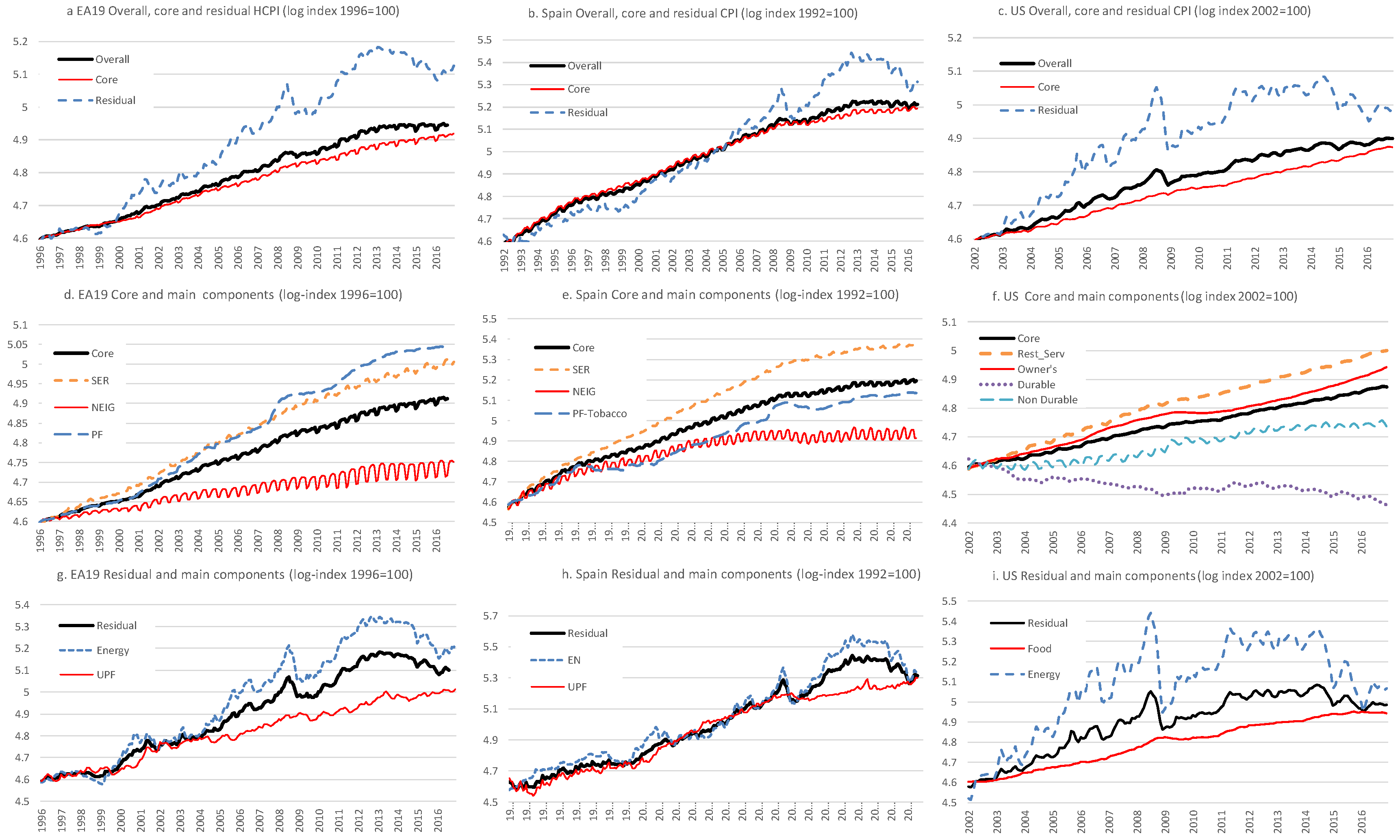
Figure 1 shows the evolution of the Harmonized Index of Consumer Prices (HICP) in the EA and CPI in Spain and US for the basic sub-aggregates. Panels a, b and c show the headline log CPI compared with core and residual inflation and they show the different behaviour between their trends and dispersion. Panels d to f refer to a decomposition of core inflation into Processed Food without Tobacco (PF*), Non-Energy Industrial Goods (NEIG) and Services (SER) for EA and Spain and in the case of US into Durable (Durable) and Non Durable (Non Durable) commodities, Owner’s equivalent rent of primary residence (Owner’s) and Other Services (Other Serv). Again we can see very different patterns in trends and also in seasonality. The same happens if we look deeper into the components of residual inflation, Energy (EN) and Unprocessed Food (UPF) or, in the US case, Food and Energy in panels g to i.

Table 2. Main statistics on basic disaggregation for annual HCPI and CPI (${\Delta }_{12}log$) for EA19, Spain and US respectively.

Disaggregates	Weight 2016	Average	Standard Deviation
Euro Area (Sample: Jan 1997–Aug 2016)
CPI	1000.00	1.72	0.93
Core	828.53	1.54	0.53
Processed Food (PF)	97.38	1.73	1.60
Tobacco (T)	23.88	4.95	2.28
Non Energy Industrial Goods (NEIG)	265.45	0.68	0.40
Services (SER)	441.82	1.99	0.58
Residual	171.47	2.52	3.87
Unprocessed Food (UPF)	74.07	2.01	2.04
Energy (EN)	97.4	2.96	6.60
Spain (Sample: Jan 1993–Aug 2016)
CPI	1000.00	2.55	1.6
Core	815.13	2.48	1.39
Processed Food (PF)	125.05	2.24	2.28
Tobacco (T)	144.8	7.02	4.84
Non Energy Industrial Goods (NEIG)	271.03	1.4	1.46
Services (SER)	399.3	3.23	1.69
Residual	184.87	2.96	4.67
Unprocessed Food (UPF)	70.3	2.82	3.05
Energy (EN)	114.57	3.08	7.69
US (Sample: Jan 2003–Dec 2016)
CPI	1000.00	2.06	1.38
Core	79.20	1.87	0.44
Non Energy Commodities less Food	19.60	0.08	1.08
Durables	9.60	ࢤ0.88	1.51
Non Durables	10.00	0.99	1.08
Non Energy Services	59.60	2.54	0.69
Owner´s equivalent rent of primary	23.10	2.28	0.94
Other Services	36.40	2.76	0.64
Residual	20.80	2.68	5.53
Food	14.00	2.44	1.51
Energy	6.80	3.17	13.45

shows the main statistics regarding the annual log difference of the CPI indexes. Columns 3 and 4 show the average and standard deviation for the period considered (January 1992–August 2016 for Spain, January 1996–August 2016 for the EA and January 2003–December 2016 for US). As can be seen, there are important differences in both the average inflation level and the standard deviations around it. Apart from Tobacco, inflation ranges from low average inflation values (0.7% and 1.4% in the EA and Spain, respectively or even negative in US, −0.99%) and low dispersion (0.4 percentage points, 1.5 p.p.) in NEIG, to high average inflation values (around 3%) and high dispersion (6.6 p.p., 7.7 p.p. and 13.5 p.p., respectively) in Energy, while Services also appear with high average inflation and low dispersion.

To discuss wider disaggregation patterns, we could start from the components’ price indexes at the maximum disaggregation level of a CPI variable, with a sufficiently large common sample. In this paper, we call them basic components.

In searching for breakdowns beyond the five basic sub-aggregates, we could start by assigning each basic component to one basic sub-aggregate1. Then, taking into account economic and institutional criteria like those listed in Table 1, we could form groups—which we call intermediate groups—of basic components in each basic sub-aggregate. The setting up of these groups should be such that their statistical properties differ substantially between groups at the time that within groups the elements are relatively homogeneous. In order to contrast it, we could aggregate the elements in each intermediate group. We call them intermediate sub-aggregates. They should show significant differences in the statistical criteria stated above. Next, for some of the above intermediate sub-aggregates, it could be useful to look for an additional breakdown. This could be done by proceeding as previously described.

The disaggregation scheme relies on in-sample characteristics, but it is always focused on its forecasting accuracy against a direct forecast. Thus, changes can happen if the forecasting accuracy deteriorates over time. In the cases of deterioration we should analyse which component is responsible and we should study if its econometric model can be improved or if this component can be successfully broken down into two or more elements. For instance, in US inflation we started working with a component which included electricity and gas, but at a certain moment the forecasts of that component were not as good as before. On studying the situation we detected that the consumer price for utility gas service was increasing much more than the electricity price and that was due to important increments in the wholesale price for gas (Henry Hub) which were not in the international prices for fuel. Consequently we began to work with two components, electricity and utility gas service.

Lorenzo (1997) did a thorough study to find an efficient disaggregation scheme of the Spanish CPI for forecasting and assessment purposes, based on economic, institutional and statistical reasons. An implication of this work is that the breakdown based on the official COICOP classification is not a very useful starting point and it is better to extend the disaggregation scheme from the five main sub-aggregates. Along this line, a wider breakdown on 30 components is proposed for forecasting Spanish inflation. In 2000, the BIAM started to publish inflation forecasts for the Euro Area using the 5-basic sub-aggregates breakdown, which was discussed and extended in Espasa et al. (2002a) and Espasa and Albacete (2007). One year earlier, the BIAM had initiated the publication of US inflation forecasts using a similar disaggregation, but with just four components—compared with Peach et al. (2013)—, because from the US CPI statistics it was not possible to distinguish between prices of processed and non-processed food. Espasa et al. (2002b) showed, by cointegration analysis and common trend analysis based on dynamic factor models that in the four mentioned components of the US CPI, there are several sources of non-stationarity. In this context, disaggregation might help to get a more accurate forecast of the headline inflation, and in their application, they show that this is the case except for very short horizons. In particular, for 12-month ahead forecasts, the reduction in RMSE with respect to a direct forecast of the aggregated CPI is more than 20%.

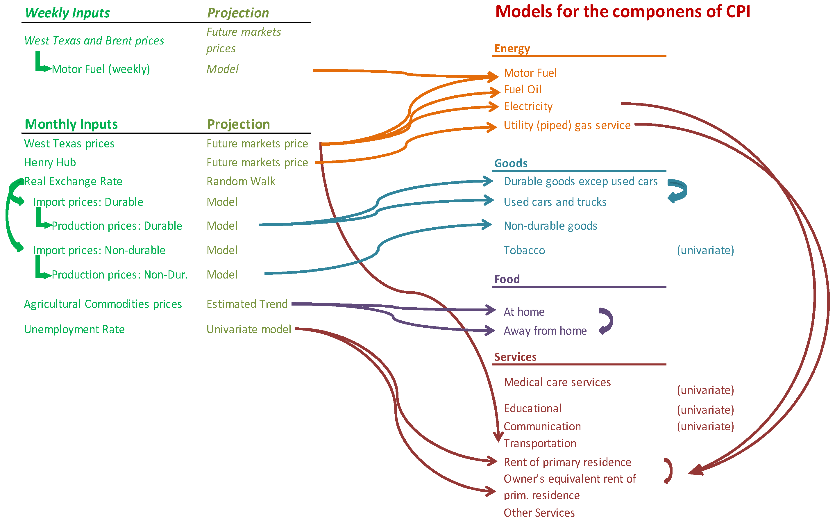
The aforementioned procedure to find a useful disaggregation can be denoted as a top-down approach and it is based on finding intermediate sub-aggregates which show clear distributional differences between them. In the formulation of the disaggregation scheme, it is also important to consider the possibility of using specific leading indicators for the models of the components or to allow that a given indicator could have different effects on them. Figure 22 shows the breakdown in 18 components used for the US CPI. In the last column, the four components which are forecast by univariate models and the indicators used in the single-equation models for the other eight can be seen. Figure 2 also points out that some components enter as explanatory variables in the models of other components.

Another disaggregation approach could be based on finding intermediate sub-aggregates which have important cross-restrictions between them. In this case, it would be of interest to study the existence of common trends. This is quite feasible when working with just the basic sub-aggregates or some aggregates from them, and successful applications can be seen in Espasa et al. (2002a), Espasa and Albacete (2007) and Peach et al. (2004). Other important cross-restrictions which might be worthwhile to study are common cycles and common breaks. For the type of reasons mentioned above, breakdowns beyond the main sub-aggregates are very appropriate. In order to find common features in the components of CPIs, Espasa and Mayo-Burgos (2013) argue that one should work the basic components, of which there are usually more than one hundred, at the maximum level of disaggregation. These authors argue that intermediate sub-aggregates based on official or ad hoc breakdowns, include, in general, a subset of basic components which share a common feature like a common trend plus other basic components which do not. Therefore, testing for common features in those intermediate sub-aggregates might not be very illustrative. In this line, Espasa and Albacete (2007) show that Core and Residual CPI in different Euro Area countries are not cointegrated. In those cases, the possible cointegration relationships present in the basic components cannot be exploited working with such intermediate aggregates. However, when working with the basic components, the number of elements is too big and a general common feature analysis is not feasible. For that reason, the BIAM methodology is not based on building from the basic components up.

In using disaggregated data from the maximum level of disaggregation, Espasa and Mayo-Burgos (2013) and Carlomagno and Espasa (2015a, 2015b) propose a limited search of common trends and cycles based on pairwise testing procedures on the basic components. In this framework, one can set up a bottom-up approach to find a useful breakdown, as opposed to the top-down approach followed in the BIAM. The bottom-up procedure is very useful when one is interested in the aggregate and all its components. Otherwise, the approach in the BIAM could be recommended.

A final issue is that the disaggregation can be performed in two main different directions: by economic sectors and by geographical areas—mainly regions in a country and countries in an economic area. What matters is to choose and implement a promising direction. The appreciation that inside a national economy, the differences between the trends, seasonality, persistence and volatility of the components could be greater in a sector breakdown than in decomposition by regions led to using the sector approach from the early stages of the BIAM. For the Harmonized Index of Consumer Prices (HICP) in the European Monetary Union, Espasa et al. (2002a) give evidence at the level of the five basic sub-aggregates that both breakdowns are useful, but the sector disaggregation improves the direct forecasts consistently through the horizons considered, while the country disaggregation shows improvements only in the very short horizons. The conclusion that the sector breakdown is more relevant—it contains more diverse information about the aggregate which is useful for the econometric analysis—than the geographical disaggregation is also obtained in Espasa and Albacete (2007) and Pino et al. (2016). Thus, the BIAM’s methodology, which follows the breakdown by sectors, is consequent with those results. With respect to this double-criterion disaggregation by sectors and regions from the basic components and according to the results in Pino et al. (2016), it can be said that their improvements on the overall inflation with respect to just disaggregating by sectors are marginal and this justifies our not making much use of it. Nevertheless, when there is a genuine interest in the results for sectors in the different regions, Pino et al. (2016) show that this analysis is not only reliable—they study a breakdown in 600 series for the EA12 and 969 for Spain—but accurate in the sense that they improve the direct forecast accuracy of the overall inflation in the case for Spain and that they are not significantly less accurate in the case of the EA12.

Though this paper focuses on inflation, BIAM also forecasts and assesses GDP. For more details on the approach followed in forecasting GDP and its components, see Minguez and Espasa (2006). These authors analyse forecasting the EA GDP by different types of econometric models, showing that the best forecasting results, from the type of models that they analyse, are obtained by combining the GDP forecasts derived from disaggregation in terms of demand components with those derived from disaggregation in terms of supply components using leading indicators in both cases.

The quarterly forecasts of the GDPs of the 17 Spanish Regions were formalized in Cuevas et al. (2015), who propose a forecasting method in which the GDP variables are disaggregated in the different official production sectors. The procedure interpolates the annual data at a quarterly level using leading indicators and builds econometric dynamic models to forecast all the quarterly production components of all GDPs of the Spanish regions; from them, corresponding regional initial GDP forecasts are obtained. The final forecasts are calculated by adjusting the initial ones to fulfil triple jointly-consistency criteria: temporal inside each region, inter-regional and non-linear to account for the linked Laspeyres indexes used in national and regional accounts.

2.4. Hierarchical Forecasts

Many economic time series can be disaggregated in a hierarchical structure taking into account some attribute. For instance, the CPI according to the COICOP classification can be disaggregated in twelve categories (sub-aggregates) denominated groups. Each group can be disaggregated in several subgroups, each subgroup in classes, and each class in several categories denoted subclasses. These subclasses correspond to what we have called basic components. These connected breakdowns could be seen as a disaggregation tree. The disaggregation trees can be more complex. For instance, in the previous example, for the Euro Area, each class could be disaggregated by countries. In hierarchical forecasting given a fixed disaggregation tree, one wants to forecast all the series in it in a consistent way. Thus, the forecast of the series corresponding to any particular knot in the tree, including the top, must sum the forecasts of the series corresponding to lower levels. This can be done top-down or bottom-up. In the first case, the procedure usually consists of forecasting the aggregate and then distributing it using historical proportions (contributions). In the second case, from the forecasts at the lowest level, the upper level forecasts are obtained by the corresponding summations. In the inflation case, the contributions cannot be considered constant and the top-down method would require forecasting the contributions by modelling them and these models could be more complex than those required in the bottom-up approach.

We have designed the disaggregation structure in the BIAM from top to bottom, but once it is fixed, the forecasting procedure goes from the established disaggregation level to the top. Thus, the forecasting procedure used in the BIAM is a bottom-up method. It has a large difference with a corresponding hierarchical approach. In the latter, the disaggregation scheme is taken as given, and in the former, we have already appreciated that formulating this scheme is an important part of the procedure and must be done taking into account different criteria as listed in Table 1. In the hierarchical approach, in principle, based on Hyndman et al. (2011), it would be possible to formulate all trees corresponding to all possible bottom lines at different levels and not necessarily homogeneous at the different branches of the tree. Then, forecasting with all possible trees (a huge number), we could determine which one generates the optimal forecast. That would be quite complex. Besides, the disaggregation structure could be difficult to interpret, while in the BIAM, the disaggregation has been guided by relevant criteria.

Finally, the hierarchical bottom-up approach also differs from the one in Espasa and Mayo-Burgos (2013) and Carlomagno and Espasa (2015a, 2015b). In the latter, the main effort lies in finding certain common trends and cycles between the basic components, such that they could be used, when appropriate, in the single-equation forecasting models for the components.

2.5. Intervention Analysis, Outlier Correction and Robust Forecasts. Breaks in Seasonality

By correcting for outliers and location shifts in the models of the components we do not need to assume normality in the data. What is required is that after these corrections the residuals are normal. Juselius (2015) argues that this is a quite general assumption in macro-economic models. In this approach, we would have a problem of special unusual events that from time to time affect the data, and they could be dealt by outlier correction. In a recent paper, Johansen and Nielsen (2016), making an important contribution to the subject by developing an asymptotic theory which applies to different outlier detection procedures, illustrate how outlier detection is very closely connected to robust statistics. Doornik and Hendry (2016) argue that model selection and robust estimation should be handled jointly and show that the impulse indicator saturation (see Chapter 15 in (Hendry and Doornik 2014)) could make that possible. In econometric modelling, the correction for outliers is essential for getting valid models, and the proposal in Doornik and Hendry (2016) is especially relevant.

In the BIAM we do not proceed as suggested by Doornik and Hendry (2016). In general, we define as an outlier a residual with an absolute value approximately greater than 2.8 standard deviations. This procedure is very usual in applied econometrics, even when it is model dependent and certainly not optimal. In our case the inconveniences of the procedure would be palliated, because once an outlier correction has been introduced in the model of a particular price component by dummy variables, those variables are kept in future revisions of the model unless they turn out to be insignificant. Besides, in the BIAM, working with disaggregated data, we apply this correction to all the series and consequently the outlier correction procedure followed is more complex and reliable than usual procedures. This is because in the BIAM we look for outliers in the components. This is laborious but, in general, it will lead to a better correction of the aggregate.

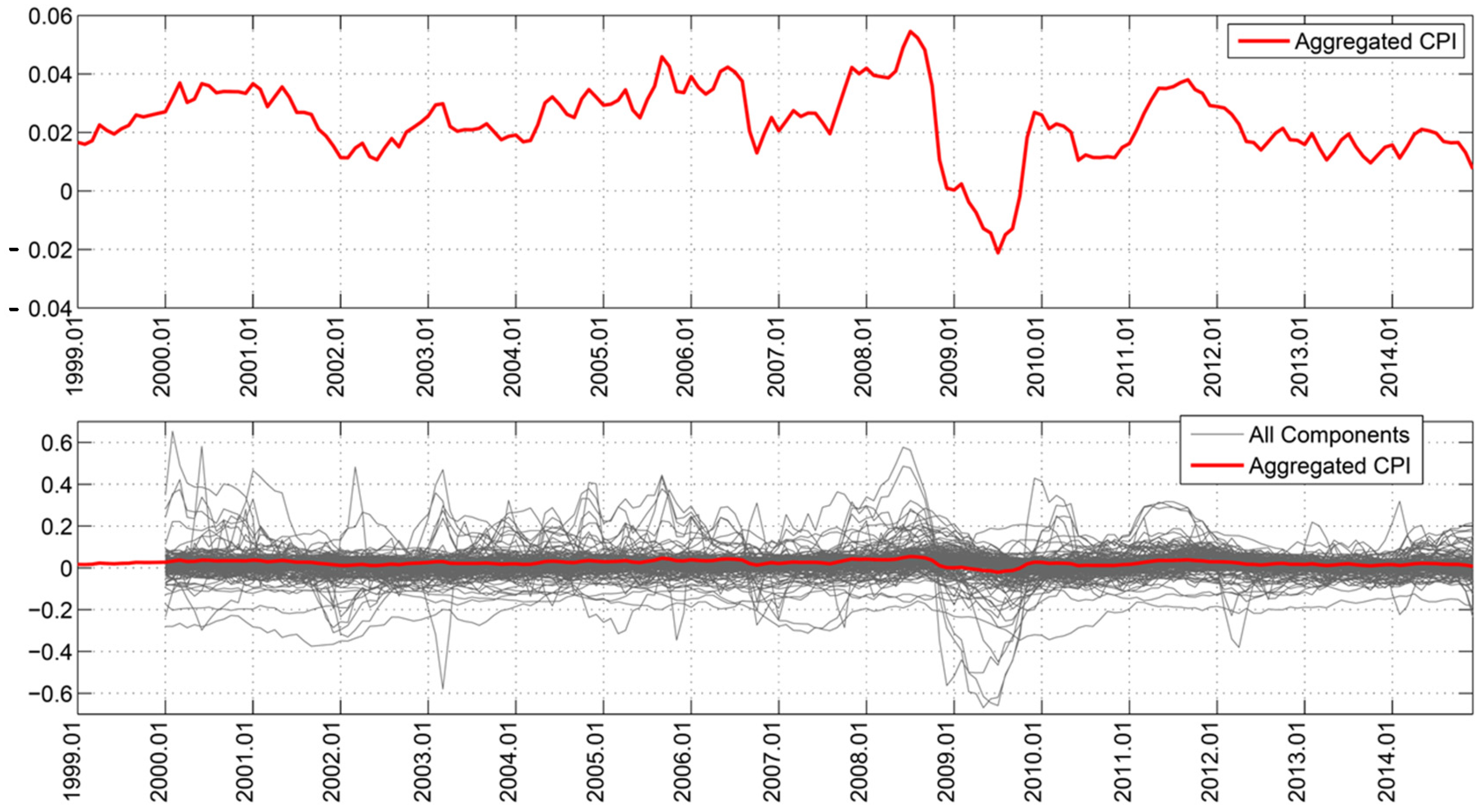
The advantages of estimating the outliers at the disaggregated level can be guessed from a plot of the headline inflation rate with its basic components. For instance, in Figure 3 (taken from (Carlomagno 2016)), which refers to the US CPI, we can observe that the historical oscillations of the y-o-y headline inflation since 1999 have been, approximately, between plus 5.7% and minus 2%, with a few relevant peaks and troughs, but we also see that there is a group of a large number of components in which we find more frequent and abrupt oscillations. Taking into account the standard residual deviations of the components’ models, and defining as an outlier a residual with an absolute value approximately greater than 2.8 standard deviations, the average number of outliers in the 164 basic components is 4.7 (2.6% of the monthly observations between January 2000 and December 2014), but in ENE and SERV, the corresponding averages are 8.2 (4.5%) and 6.5 (3.6%), respectively. The number of large outliers (greater than 4 standard deviations) is 37% of the total of outliers. From Figure 3, it could also be derived that the number of highly contaminated series (series with 5% or more outliers in the sample) is 21 out of the 164. Finally, analysing the outlier congestion indicator, whose values in each month of the sample are the number of basic components with at least one outlier in this month, Carlomagno (2016) shows it has seasonality with a peak in January and a mean shift during the sub-prime crisis.

The description above for the US CPI points out how promising it could be to deal with outlier corrections of this aggregate from the components. In fact, working with this variable, Carlomagno (2016) proposes constructing an aggregate indicator for its outlier correction by aggregating the estimated outlier effects in the components. The indicator provides a better correction in the aggregate than a direct correction. Since the DGP for the US CPI includes all the basic components, any outlier in them is an outlier in the aggregate, even when in the aggregate many of them could not be estimated. For all those reasons, the outlier corrections in the BIAM are applied at the disaggregated level, which in any case is a natural consequence of modelling from a breakdown of the aggregate.

Besides, with this approach, it would be easier to detect whether an outlier corresponds to a specific event, in which case it could be possible to model its effects with more information. BIAM history is full of this kind of example, showing that for identification, estimation and diagnosis purposes, the outlier corrections would be better performed from disaggregated data. For instance, in analysing the HCPI of the Euro area, in the BIAM corresponding to September 2003, the last forecast error in the headline inflation was not significant, but the error in the SERV component was. Looking for factors which could generate this error, it was necessary to go to detailed data by countries. It was found that the error came from the behaviour of recreational and cultural service prices and restaurants and hotel prices in Germany, which had changed their seasonal pattern in 2000. With this information, the model for SERV for the Euro Area was reformulated, and in the new model, the indicator variables for Easter and the “Euro rounding effects” also changed their coefficients and the whole fit improved significantly (see also EFN 2013).

With the disaggregated approach we have, when analysing the forecast error for headline inflation from the last observation before updating the forecast, we could look for forecast errors significantly different from zero in the components even when the error in the aggregate is not. In any case, in doing so, we would be able to correct the outlier in the specific components of the aggregate that require intervention, as we have seen in the previous paragraph.

Eurostat regulations for HICP construction at the member-state level have changed the seasonality of some price indexes and consequently of the aggregate on a couple of occasions–see NEIG components in Figure 1. This occurred when Eurostat regulated the prices of sales to be included in the HICPs and, when required, the prices of seasonal goods to be considered also in the months in which they do not appear in the markets, taking into account the prices of other goods from the same COICOP group. In our experience, in which we need to forecast till 24 months ahead, the question of which is the best way of modelling seasonality, by dummy variables or by annual-differences, has not a definite answer, and it is something that should be tested in each case. This is in line with the results in Osborn et al. (1999) and Osborn and Clements (2002). However, when there are seasonal breaks, the seasonal patterns are better modelled using specific seasonal dummies for each period of stable seasonality. This modelling is done only for the components affected by the Eurostat regulations, for instance, clothing and footwear. Proceeding in this way in the BIAM we are able to assign the appropriate seasonal change in the indirect forecast of the headline inflation.

2.6. Linking the Forecasts from Leading Indicator Models with Those from Congruent Econometric Models

The procedure in the BIAM is based on single-equation models with leading indicators and consequently does not provide a causal explanation of the observed and forecast inflation. If the number of components is not large, our procedure can be extended to include causal explanatory variables in the different models (see (Aron and Muellbauer 2012)). However, if the number of components is high, an alternative approach is required. The following suggestion is based on relating forecasts from disaggregated component models to those of a congruent econometric model for the aggregate. The first approach usually makes use of relevant monthly information about different price trends, cycle, seasonality, breaks, etc., along markets, and in many instances it will be more accurate in forecasting. The econometric model for the aggregate will be much more informative on the causes of inflation. In order to borrow a causal explanation for the inflation forecasts obtained in the BIAM, we have proceeded as follows. First, we perform a simple regression between these forecasts, y_t, and the forecasts that result from a macroeconomic model, x_t, denoted as congruent econometric forecasts.

y_t = c + bx_t + r_t.

It should be noted that inflation is I(0) and, so are the forecasts. Thus, we can test the null that c equals zero and b equals one. If the null is not rejected, we can substitute the x_t forecasts in the regression above for their composition in terms of the explanatory variables used to calculate them. Thus, we borrow a causal explanation for the inflation forecasts (y_t). The component r_t (the part of the disaggregated forecasts which is not explained by the econometric forecasts) could be interpreted as the impact of the heterogeneous inflation situation in the different markets on total inflation. The above test is not a real encompassing test and neither is it a test for causality, but it can be seen as a test for efficiency. The variance of the forecasting errors of y_t is smaller than the variance of the errors of x_t. With this result it could be considered that the superior forecasts are compatible with the explanation in terms of regressors of the alternative (direct) forecast and, consequently, that explanation could be borrowed even when others are possible. In any case, if the analyst was prepared to use the explanation in the direct forecast, this regression procedure which exploits the variance dominance of the indirect disaggregated approach could be more appealing.

An application of this procedure can be seen in European Forecasting Network (EFN 2013, Annex Chapter 1.a. Box 4. pp. 9–10). The estimated regression was:

$$\begin{array}{c}{y}_{\mathrm{t}}=0.95x_{\mathrm{t}}+r_{\mathrm{t}}\\ \left(0.07\right)\\ \mathsf{\sigma }\left(r_{\mathrm{t}}\right)=0.001,{\mathrm{R}}^2=0.99\end{array}$$

where y_t are the BIAM indirect forecasts and x_t the congruent econometric forecasts of headline inflation, both in quarterly values. This regression shows that specific forecasts could differ considerably, with a 95% confidence interval given by ±0.2 percentage points. The explanatory variables in the model (see Dreger 2002 and Dreger and Marcellino 2007) for x_t are the deviations from two long-run restrictions, one linking prices with unit labour cost and another with money. Other explanatory variables are changes in import prices, the output gap and lagged inflation values. The forecasts y_t are more accurate than x_t, and besides, using the equation above, the y_t forecasts inherit a causal explanation from x_t. In this example, we can say, as stated in the above report, “that the amount of money in relation to output is pushing inflation up, that unit labour cost and output gap are pushing in the opposite direction and that the heterogeneous inflation situation on different markets is favouring lower inflation rates”. Based on these results, the report concluded that a loose monetary policy at that time could continue.

3. The Assessment of Inflation and Inflation Expectations: An Application of the BIAM Methodology

Having discussed the methodology developed in the BIAM and its connection to the literature, in this section we present how this methodology can be used to assess inflation and inflation expectations. We do it illustrating how it has been done in the BIAM.

Based on the observed data of a given CPI breakdown and their previous corresponding forecasts, the assessment of inflation and inflation expectations is done through: (1) evaluating the new published data; (2) updating short and medium- term projections and also comparing them with previous ones and, if possible, by providing hints about the causal variables behind those projections; (3) using quantitative measures of the uncertainty around the forecasts; and (4) using the detailed components’ forecasts. With all those ingredients, a diagnostic is derived.

The possibility of obtaining hints about causal variables in the BIAM procedure is based on the fact that the headline inflation could have similar rate values at two time moments, but the inflation situations could be quite different because the variables causing inflation in these cases differ substantially. As mentioned in Section 2.2, inflation at the sector level is determined by distinct variables or by the same ones with very diverse impacts. In particular, certain facts apply. (1) Different international commodity prices affect some sectors—usually processed food and energy—more than others, in which case the models of the former sectors include some international prices as leading indicators. (2) Technological changes are not equally important and frequent in the production of the different sectors and, therefore, in their prices. Thus, technological innovations are more often in non-energy industrial goods than in other goods or services. (3) Customers’ preferences change very distinctly for different products. (4) Indirect taxation is not uniform through sectors. Therefore, when analysing, at a given moment, especially high or low headline inflation values or the corresponding significant forecast errors, we could look at the break-down by sectors of these values. This disaggregation would point to the more important sectors in the determination of these special values. Thus, on some occasions the nature of these sectors and the presence of certain facts like the ones mentioned above could point to the type of causal variables behind those headline inflation values. Some examples could be as follows. Suppose that at time t we observe a high headline inflation value outside the standard confidence intervals of its corresponding forecast. Then we could look at which basic sub-aggregates it comes from. If we find that it is due to high increases in the consumer prices of certain food or energy products, we could then analyse the behaviour of the leading indicators in the models of the referred consumer prices. If it turns out that the increases in those domestic prices are mainly due to big increments in international fuel or food commodity prices we have a strong hint that the causal variable behind this high headline inflation value is foreign inflation. Another case could emerge, if when observing a significantly low headline inflation rate we detect that it comes from low values in the price indexes corresponding to the rent of primary residence and owner’s equivalent rent of primary residence. Then, we have a hint that the deflationary pressures are not due especially to foreign explanatory variables but to domestic ones coming from the building sector.

Besides, in all those situations, by updating our forecasts for the next two or three years we will be providing an estimation of the future effects of the significant innovations in the last observation detected in specific sectors.”

3.1. Evaluating New Data: The Information Content in the Forecast Error

The evaluation of new data is done by means of forecasting errors—the differences between observed and forecast values—. If the econometric models are reliable, these errors give an estimation of the innovation component of the new data. Policy makers, investors, etc., do not react to observed values but to their innovation content.

Table 3. Evaluation of data innovations. Euro Area observed and expected monthly rates, October 2016.

Basic Sub-Aggregates	Weights 2015	Observed	Forecasts	Confidence Intervals *
Processed Food	122.72	0.09	0.09	±0.38
Tobacco	23.94	0.04	0.47
Processed food excluding tobacco	98.78	0.10	0.02
Non-energy Industrial goods	266.60	0.64	0.65	±0.21
Services	427.76	−0.18	−0.12	±0.14
Core	817.08	0.13	0.15	±0.13
Non-processed food	74.85	−0.03	0.84	±0.72
Energy	108.07	1.60	1.30	±0.86
Residual	182.92	0.88	1.07	±0.57
Overall	1000.00	0.25	0.31	±0.12

* Confidence intervals at 80% calculated with historical errors. Source: Eurostat & BIAM (UC3M). Date: 17 November 2016.

, which corresponds to Table I.2.3 in BIAM 266 (2016), helps to understand the role of the forecasting errors in the assessment of inflation, by illustrating the analysis with the figures for October 2016 in the EA. The table includes the observed monthly inflation rates on that date (column 3), the one- month ahead forecasts available with information up to September (column 4), and the 80% confidence intervals calculated with the historical one-step ahead forecast errors made in BIAM (column 5). The differences between the observed values and one-step ahead forecasts are a highly relevant measure for assessing current inflation data. Thus, the comparison of this forecast error with the corresponding confidence interval allows us to detect whether there is any significant innovation in inflation.

Table 3 shows the forecast error for headline inflation and for the basic sub-aggregates. This table allows us to detect any significant innovation and the sub-aggregate of provenance. As can be seen in Table 3, on this occasion, there were no significant innovations except for NPF. The analysis of the forecast errors at a more disaggregated level of 30 components—using auxiliary ARIMA models—signalled that such a negative error was not general in the components of this sub-aggregate. It came exclusively from prices of fresh fruit, pulses and vegetables. In summary, Table 3 allows us to know the magnitude and origin of the innovations, which turned up in the last observed data, providing useful information to interpret the data and to apply a precise revision of the model if needed. It must also be noted that an unexpected shift in inflation can be very badly approximated by a high value of the price increment of a component with respect to the others; we need to compare it with the forecasting interval. The analysis of the forecast errors which are significantly different from zero allows us to perform a quantitative modelling of these outliers by including, if possible, omitted variables or by applying mean corrections or using robustified forecasting procedures—see Hendry (2006) and Castle et al. (2015). In this case, we applied dummy variables in the two price indexes affected, fruits and vegetables, estimate the outlier effect in both series, construct a weighted average of them and use it to correct the outlier in the model for NPF. In this way the last innovation in NPF is not forced to be zero.

3.2. Updating Forecasts

Once the forecast errors have been analysed and the models have been corrected, if necessary, the BIAM reports new updated path forecasts for inflation in the headline index, core, residual and basic sub-aggregates. The importance of these updates can be evaluated in two coincident ways. They can be seen as a full assessment of the current situation and as a formulation of future expectations. In fact, present values of the components of the CPI include recent innovations which, given the nature of those variables, are going to have necessarily future effects on most macro variables. Consequently, the present inflation situation is not properly understood if we do not estimate the future projection imposed by the hidden innovations. In that sense, working with appropriate models, the forecasts, as the inherent projection of the present, are never wrong. In their second meaning, those projections are in fact our expected future values. However, the future values will also be affected by future unforecastable innovations, and the forecasts made will, in general, depart from those observed values, generating forecasting errors. They are also very useful, because they capture only the innovation components in those observations. It is also interesting to see that even if one is only interested in a forecast h periods ahead, the information about the path with which this forecast is attained is still usually relevant. It could be quite different to attain this future value from a path above it than from a path from below.

Table 4. Updating forecasts: Inflation forecasts in the Euro Area (Forecasts since January 2017).

		Core							Residual			Total HICP	80 % Confidence Interval
		Processed Food Excluding Tobacco	Tobacco	Non Energy Industrial Goods	Services	Total CORE	80 % Confidence Interval		Non Processed Food	Energy	Total Residual
Weights 2016		9.9%	2.4%	26.7%	42.8%	81.7%			7.5%	10.8%	18.3%
	Annual Average
	2015	0.0	3.0	0.3	1.2	0.8			1.6	−6.8	−3.4	0.0
	2016	0.1	2.3	0.4	1.1	0.8			1.4	−5.1	−2.3	0.2
	2017	0.1	2.3	0.3	1.2	1.0	±	0.33	1.9	6.7	4.7	1.6	±	0.65
	2018	1.4	4.0	0.5	1.0	1.0	±	0.42	2.6	2.9	2.8	1.3	±	0.80
	ANNUAL RATES (year-on-year rates)
2016	July	0.0	2.4	0.4	1.2	0.8			2.9	−6.7	−2.7	0.2
	August	0.0	2.3	0.3	1.1	0.8			2.5	−5.6	−2.2	0.2
	September	0.0	2.3	0.3	1.1	0.8			1.1	−3.0	−1.3	0.4
	October	0.1	2.3	0.3	1.1	0.7			0.2	−0.9	−0.4	0.5
	November	0.3	2.3	0.3	1.1	0.8			0.7	−1.1	−0.3	0.6
	December	0.3	2.5	0.3	1.3	0.9			2.1	2.6	2.4	1.1
2017	January	0.3	2.9	0.3	1.2	0.8	±	0.13	2.6	7.7	5.5	1.7	±	0.14
	February	0.5	3.1	0.2	1.3	0.9	±	0.19	2.6	8.2	5.8	1.8	±	0.27
	March	0.7	3.2	0.2	1.0	0.8	±	0.24	2.2	7.6	5.2	1.6	±	0.38
	April	0.7	3.1	0.3	1.5	1.1	±	0.28	2.1	7.9	5.3	1.8	±	0.50
	May	1.1	2.7	0.3	1.3	1.0	±	0.33	1.6	6.3	4.2	1.6	±	0.60
	June	1.2	2.8	0.4	1.2	1.0	±	0.37	1.8	5.0	3.7	1.5	±	0.70
	July	1.4	3.2	0.4	1.2	1.0	±	0.42	1.1	6.3	4.1	1.6	±	0.79
	August	1.4	3.3	0.4	1.2	1.0	±	0.47	1.0	7.7	4.8	1.7	±	0.88
	September	1.6	3.4	0.2	1.2	1.0	±	0.53	2.1	7.0	4.9	1.7	±	0.97
	October	1.6	3.9	0.4	1.2	1.1	±	0.57	2.1	5.7	4.2	1.7	±	1.04
	November	1.4	4.1	0.4	1.2	1.1	±	0.61	2.1	6.4	4.6	1.7	±	1.11
	December	1.5	4.2	0.5	1.2	1.1	±	0.65	1.6	4.9	3.5	1.5	±	1.17
2018	January	1.5	4.2	0.3	1.0	0.9	±	0.68	1.6	2.7	2.3	1.2	±	1.23
	…	…	…	…	…	…			…	…	…	…
	December	1.3	3.9	0.4	1.2	1.1	±	0.69	3.0	2.1	2.4	1.3	±	1.25

Source: Eurostat & BIAM (UC3M). Date: 18 January 2016.

, corresponding to EA inflation, shows annual and monthly y-o-y rates for the past and future values of inflation since January 2017. In average annual rates, Table 4 collects the observed rates for the previous nine years and the corresponding forecasts for the current year and the next two years. For monthly y-o-y rates, the table includes the observed rates for the current year and their forecasts for the remaining months of the year and for those of the next two years. For all of them, the average and y-o-y forecasts, the table provides 80% confidence intervals for headline and core inflation. Thus, on a single page the user has the most relevant forecasting results. The BIAM also reports on month-on-month rates in a table similar to the previous one.

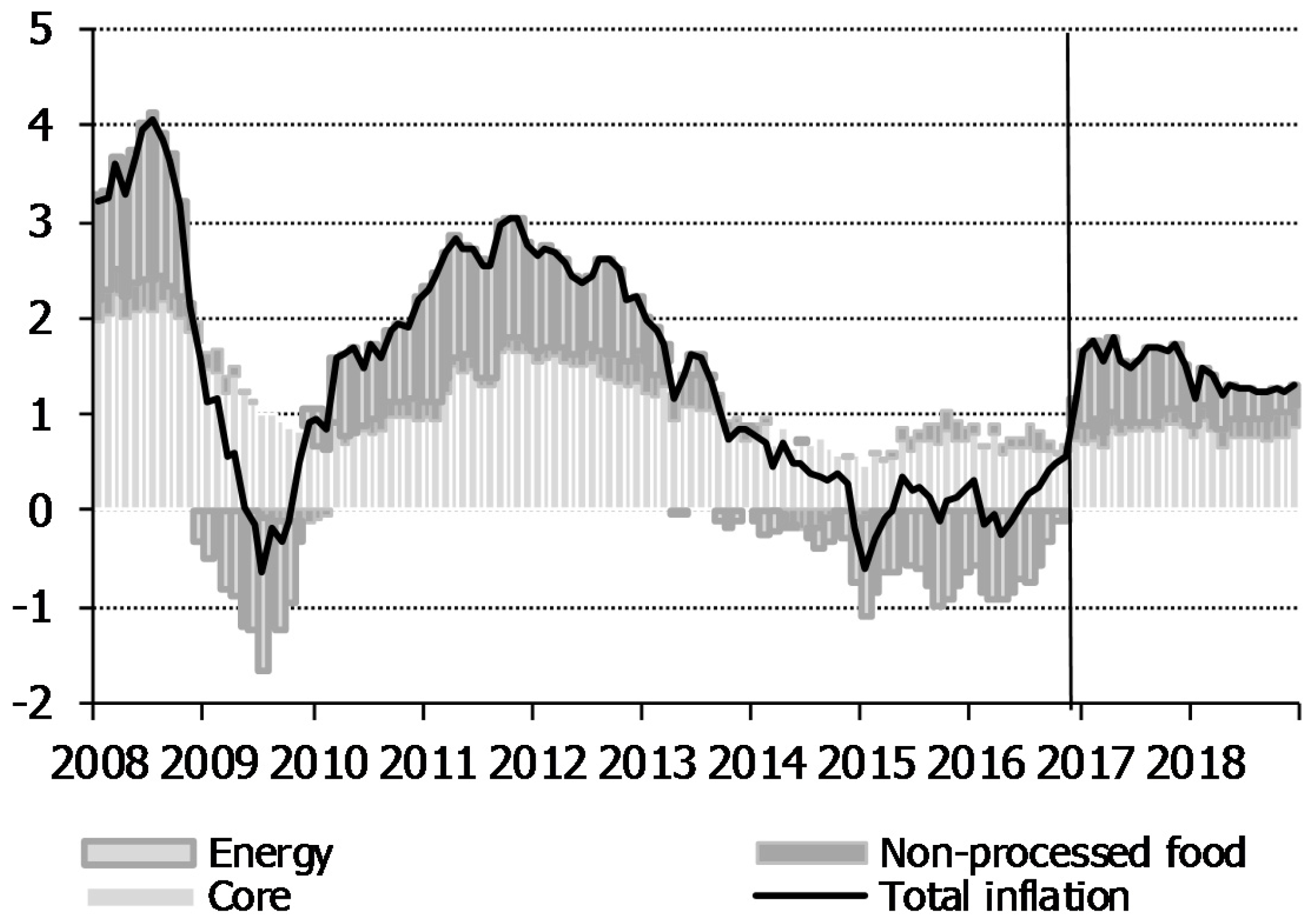
To assess the relevance of changes in core and residual inflation on headline inflation, the information in Table 4 is complemented with their contributions. Figure 4 shows the contribution of core and residual inflation on headline inflation. This graph points out that core inflation is less volatile and more persistent than residual inflation. Figure 4 helps to understand that the period of almost zero or negative headline inflation, which goes from the end of 2014 to near the end of 2016, is a period of negative contribution from energy prices. However, it was also a period of stable low core inflation around 0.8%, which might have been the main concern for the ECB.

3.3. Using Quantitative Measures of the Uncertainty around the Forecasts

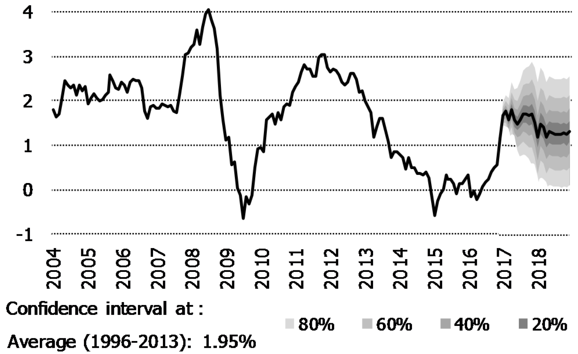
Measuring uncertainty plays a key role in the assessment of a future path of inflation. In the BIAM, an important effort has been made from its beginning in 1994 to provide different confidence intervals. Since May 2003, it has provided such intervals for all future data points; see Figure 5. This type of plot is known as a fan chart and was introduced by the Bank of England in its quarterly report of February 1996; see Britton et al. (1998) and Wallis (1999). Different ways to construct these charts have been reported in the literature. In the BIAM, they are calculated assuming normality and using own historical forecasting errors to calculate the standard deviations for the different horizons. Figure 5 (see also Table 4) shows the estimated fan chart with information up to December 2016 as published in the BIAM. Using the same information Table 4 shows that the expected headline annual average inflation rate for 2017 will be around 1.6% with an 80% confidence interval whose amplitude is of plus-minus 0.65 percentage points (p.p.). The corresponding values for 2018 are 1.3% ± 0.80 pp. Combining the information from Figure 4 and Figure 5, it can be seen that the contribution of core inflation drives the mentioned behaviour of headline inflation in those years, with y-o-y rates around 1%, remaining below 1.7%, the mean value observed from 1996 to 2013.

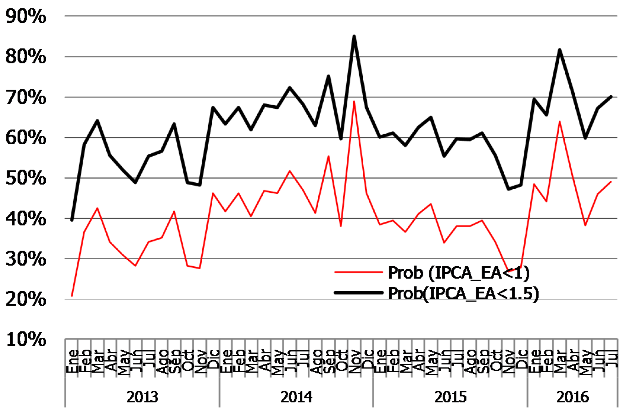
The estimated uncertainty of the forecasts also allows us to know the probability of future values that are used as benchmarks in policy. In this sense, given that the ECB inflation target is set on keeping inflation near but below 2%, it becomes relevant to know the probabilities related to attaining it in the near future. The first thing to note is that for assessing today the attainability of the target m months or y years ahead, the band of values with which it has been defined is too narrow relative to the usual oscillation of the targeted variable as it can be appreciated in Figure 5. As it could be expected, the relatively narrowness of the target increases in the medium term as is also shown in Figure 5. Therefore it seems useful to provide probabilities of ranges of values which could be a clear sign of departing from the target from above or below. In this sense Figure 6 shows the evolution of the probability that the one year ahead inflation rate (y-o-y) is below 1.5% and 1%. At the present inflation situation, the ranges of values have been chosen from below the target. In another occasions, as the year 2008, the ranges would be selected from above. High probabilities for the ranges of values reported in Figure 6 are more indicative of the difficulty of attaining the target —in this case one year ahead—, than the probabilities corresponding to the interval target.

3.4. Use of Detailed Component Forecasts

The inflation reports in the BIAM are adapted to the different economic areas that are analysed. In this sense, it publishes what could be considered a relevant disaggregation in each area and focuses on alternative inflation variables depending on the Central Bank inflation targets. In all cases, the disaggregation goes beyond the basic sub-aggregates. In Figure 2, we saw the disaggregation used in the BIAM for US inflation. First, notice that the BIAM definition of US Core inflation in the CPI is the one used by BLS, not coinciding with the one used in the EA and Spain. Second, the basic disaggregates are also different. Nevertheless some characteristics are common. Thus, in all the economic areas, services are the most inflationary basic component in Core inflation, as seen in Table 2. In many occasions it is of interest to see which sectors in the basic sub-aggregates show relative relevant behaviours, for instance in terms of higher or lower inflation rates. As an example, in November 2016 in US, using data for the breakdown as in Figure 2,—see table II.2.3 in BIAM 266—the components in the Core with higher inflation forecasts were prices related to rents and medical services. Also another interesting result in this referred table corresponds to inflation on durable goods, which was projected with persistent negative rates, while the rates of non-durables show positive ones, possibly due to a different impact of the technological innovations in these two types of goods.

On the other hand, as inflation forecasts are a relevant input for monetary policy, it is useful to analyse and forecast the CPI and other possible inflation variables on which the corresponding central bank formulates its inflation targets. For that reason, the BIAM in the case of the US also includes forecasts for the core personal consumption expenditure index, PCE, and for the market-based PCE, as can be seen in

Table 5. US inflation by components and alternative measures of core inflation (Forecast values since January 2017).

		CPI
		Overall CPI	Confidence Intervals at 80% Level		CORE CPI	Confidence Intervals at 80% Level		PCE CORE	MB-PCE
	Weights 2016	100%			79.2%
	Annual Average
	2015	0.12			1.83			1.4	1.0
	2016	1.26	±	0.01	2.21	±	0.01	1.7	1.4
	2017	2.13	±	0.54	2.22	±	0.23	1.8	1.8
	2018	1.97	±	0.65	2.27	±	0.30	2.0	1.9
	ANNUAL RATES (year-on-year rates)
2016	July	0.8			2.2			1.6	0.8
	August	1.1			2.3			1.7	0.8
	September	1.5			2.2			1.7	1.0
	October	1.6			2.1			1.8	1.2
	November	1.69			2.11			1.65	1.50
	December	2.03	±	0.11	2.18	±	0.09	1.71	1.50
2017	January	2.3	±	0.35	2.2	±	0.16	1.6	1.9
	February	2.8	±	0.57	2.1	±	0.21	1.6	2.0
	March	2.4	±	0.69	2.2	±	0.26	1.8	2.3
	April	2.0	±	0.74	2.2	±	0.30	1.7	2.3
	May	1.8	±	0.79	2.1	±	0.32	1.7	2.3
	June	1.8	±	0.83	2.2	±	0.34	1.8	2.3
	July	1.9	±	0.89	2.3	±	0.34	1.8	2.3
	August	2.1	±	0.94	2.2	±	0.35	1.8	2.3
	September	2.1	±	0.96	2.3	±	0.36	1.9	2.3
	October	2.2	±	0.97	2.3	±	0.39	1.9	2.3
	November	2.1	±	0.98	2.3	±	0.43	2.0	2.3
	December	2.1	±	1.01	2.3	±	0.43	2.0	2.3
2018	January	2.0	±	1.04	2.3	±	0.42	2.0	2.3
	…	…		…	…		…	…	…
	December	2.0	±	1.07	2.3	±	0.41	2.0	2.3

Source: Federal Reserve & BIAM (UC3M). Date: 15 December 2016.

.

Finally, the breakdown at the maximum disaggregation level turns also to be very useful and informative. Thus, in the Spanish case, besides the selected breakdown in 30 components, the BIAM also provides forecasts for the CPI components at the maximum level of disaggregation—basic components. In this case, they are obtained by univariate models and then restricted to guarantee that the headline forecasts from those 111 items coincide with the ones obtained by the more elaborated procedure from the 30 components.

Table 6. Consumer Price Index by subclass and special group in Spain.

Item	Weight (%)	2016	2017	Item	Weight (%)	2016	2017	Item	Weight (%)	2016	2017
NON-ENERGY IND. GOODS (NEIG)	26.42	0.6	0.6	PROCESSED FOOD AND TOBACCO (PF)	15.13	0.2	0.2	SERVICES (SERV)	39.67	1.1	1.0
Men’s outerwear	−0.05	−1.4	1.4	Rice	−0.94	1.2	−1.8	Maint. & rep. srv.	0.28	1.9	0.4
Men’s underwear	0.09	−1.1	2.4	Flours & cereals	-0.34	−0.2	0.2	Ot. srv. related to vehicles	−0.04	0.6	−1.4
Women’s outerwear	−0.15	−1.7	0.2	Bread	−0.03	−0.1	−0.4	Railway transport	0.49	1.3	0.8
Women’s underwear	0.09	−0.9	2.1	Pastry goods, cakes etc.	−0.01	0.5	0.4	Road transport	0.17	1.4	−0.1
Child. & inf. garments	−0.02	−1.7	1.0	Farin.-based prd.	−0.16	0.9	−1.8	Air transport	0.06	−2.7	0.1
Men’s footwear	0.01	1.0	1.3	Delicat. type meat prd.	0.00	−0.1	−0.4	Ot. transport srv.	0.55	−0.6	2.2
Women’s footwear	0.10	1.0	1.8	Processed meat prd.	−0.08	0.5	0.3	Insur. con. with transport	0.18	3.6	2.6
Child. & inf. footwear	0.01	0.9	1.4	Preser. & proc. fish	0.00	1.8	3.0	Rest, bars, coffee bars etc.	0.13	1.0	1.1
Motor vehicles	−0.12	3.6	2.9	Milk	−0.52	−3.2	−1.5	Hotels & ot. lodgings	0.02	2.6	3.4
Ot. vehicles	0.00	1.7	0.1	ot. dairy prd.	−0.33	0.1	−0.9	Package holidays	−0.46	−1.3	−0.5
Spare parts & maint	0.13	−1.8	−0.6	Cheeses	−0.02	0.2	0.2	Higher education	0.33	−0.1	0.7
Mat. f maint. & rep. dw.	0.14	−0.4	0.0	Preser. Fruits & dri. Fru.	−0.14	4.2	0.4	Postal srv.	0.45	1.5	1.4
Water supply	0.21	−0.4	0.7	Dried pulses & veg.	−0.08	7.4	3.5	Telephone srv.	−0.04	2.3	1.2
Furniture	0.11	−0.1	0.3	Frozen & preser. veg.	−0.10	1.1	−0.4	Rentals f housing	0.11	−0.8	0.0
Ot. Equip.	0.04	1.1	0.8	Sugar	−0.90	−0.3	−2.5	Srv. maint./ rep. of the dw.	0.04	−0.2	0.6
Hhold textiles	0.02	−1.3	−1.1	Choco. & confec.	−0.01	1.4	0.4	Sewerage collection	0.30	1.1	0.9
Refr.,w. mach. & dishw.	−0.18	−3.6	−3.6	Ot. food prd.	0.02	0.2	−0.4	Out. Hosp. & param. srv.	0.14	0.5	1.4
Cookers & ovens	−0.16	−0.6	−1.7	Coffee, coc. & infus.	−0.01	−0.1	−0.1	Dental srv.	0.13	0.9	0.7
Heating & air cond.	0.07	−0.4	−0.5	Min. waters. drinks etc.	−0.23	1.8	0.3	Hospital srv.	−0.08	−2.1	−1.3
Ot. hhold app.	0.05	−1.6	−1.7	Spirits & liqueurs	0.17	0.2	1.4	Medical insurances	0.56	4.4	4.1
Glass.,crock. & cutlery	0.19	0.0	0.6	Wines	−0.08	1.0	0.5	Recreational & sporting srv.	0.11	1.0	1.5
Ot. kitchen uten. & furn.	0.22	0.5	0.2	Beer	0.07	0.5	1.0	Cultural srv.	0.16	0.4	0.6
Tools & acc. f h. & gard.	0.23	−0.4	−0.2	Tobacco	1.50	0.4	1.3	Education	0.21	0.9	1.1
Cleaning hhold art.	−0.08	−0.3	0.1	Butter & margarine	−0.16	−0.6	1.3	Rep. of footwear	0.35	1.4	0.6
Ot. non-dur. hhold art.	0.11	0.4	0.8	Oils	−0.28	10.0	−0.7	Dom. Serv /ot. hhold srv.	0.19	0.6	−0.6
Med. & ot. pharma prd.	−0.53	−1.8	−1.3	NON-PROC.FOOD (NPF)	15.13	1.4	1.6	Insur. Con. with dw.	0.36	3.1	2.1
Therapeutic app. & eq.	0.00	−1.5	−0.2	Beef	0.05	0.3	0.5	Personal care srv.	0.14	0.9	0.3
Equip. sound & pict.	−0.86	−5.6	−5.8	Pork	−0.21	−1.5	0.2	Social srv.	0.25	0.7	0.6
Photo & cinema eq	−1.40	−3.0	−8.9	Sheep meat	−0.31	−0.7	0.2	ot. insurances	0.26	2.9	2.7
Info proc. Eq	−0.61	−9.9	−10.4	Poultry	−0.40	−1.9	−0.2	Financial srv.	0.51	0.0	−0.3
Recording media	−0.01	−3.7	−0.9	Ot. meats & n-meat ed.	−0.26	1.7	2.2	Ot. srv.	0.06	0.4	1.5
Games & toys	−0.25	−3.7	−3.5	Fresh fish	0.13	4.3	1.7	Rep. of hhold app.	0.29	0.2	0.3
Ot. Recr. & sport. art.	−0.01	−2.2	−0.1	Crustaceans & molluscs	0.32	4.9	4.1	ENERGY (ENE)	12.14	−8.6	13.7
Plants, flow. & pets	0.21	0.9	1.4	Eggs	−0.03	−0.5	−1.3	Electricity & gas	0.42	−9.9	17.1
Books	0.12	0.3	0.4	Fresh fruits	−0.12	5.5	−0.8	ot. fuels	2.47	−16.3	28.4
Newspapers & mag.	0.26	1.2	3.3	Fresh pulses & veg.	0.13	0.0	6.4	Fuels & lubricants	1.69	−7.1	10.4
Stationery mat.	0.17	0.4	0.7	Potat. & proc. prd.	0.76	12.5	−0.4
Personal care art.	0.00	−1.4	−0.6
Jewel, clocks & watches	1.25	1.9	3.4
Ot. art. f pers. use	0.04	−1.2	0.6
						2016	2017	Forec.> CPI + 80% RMSE
				Forecast CPI		−0.2	2.2	Forec.= CPI + − 80% RMSE
				RMSE 80%		0.0	1.2	Forec.< CPI − 80% RMSE

Source: INE & BIAM (UC3M). Date: January 13, 2017.

includes forecasts for the average annual rates of growth in 2017 for 111 items. The table also includes a colour code signal that allows for a quick understanding of the different inflation situations in the components. Forecasts are coloured in red when they are above the value of the upper bound of the confidence interval at 80% for the headline inflation, in green when they are below and in yellow when they are in the interval.

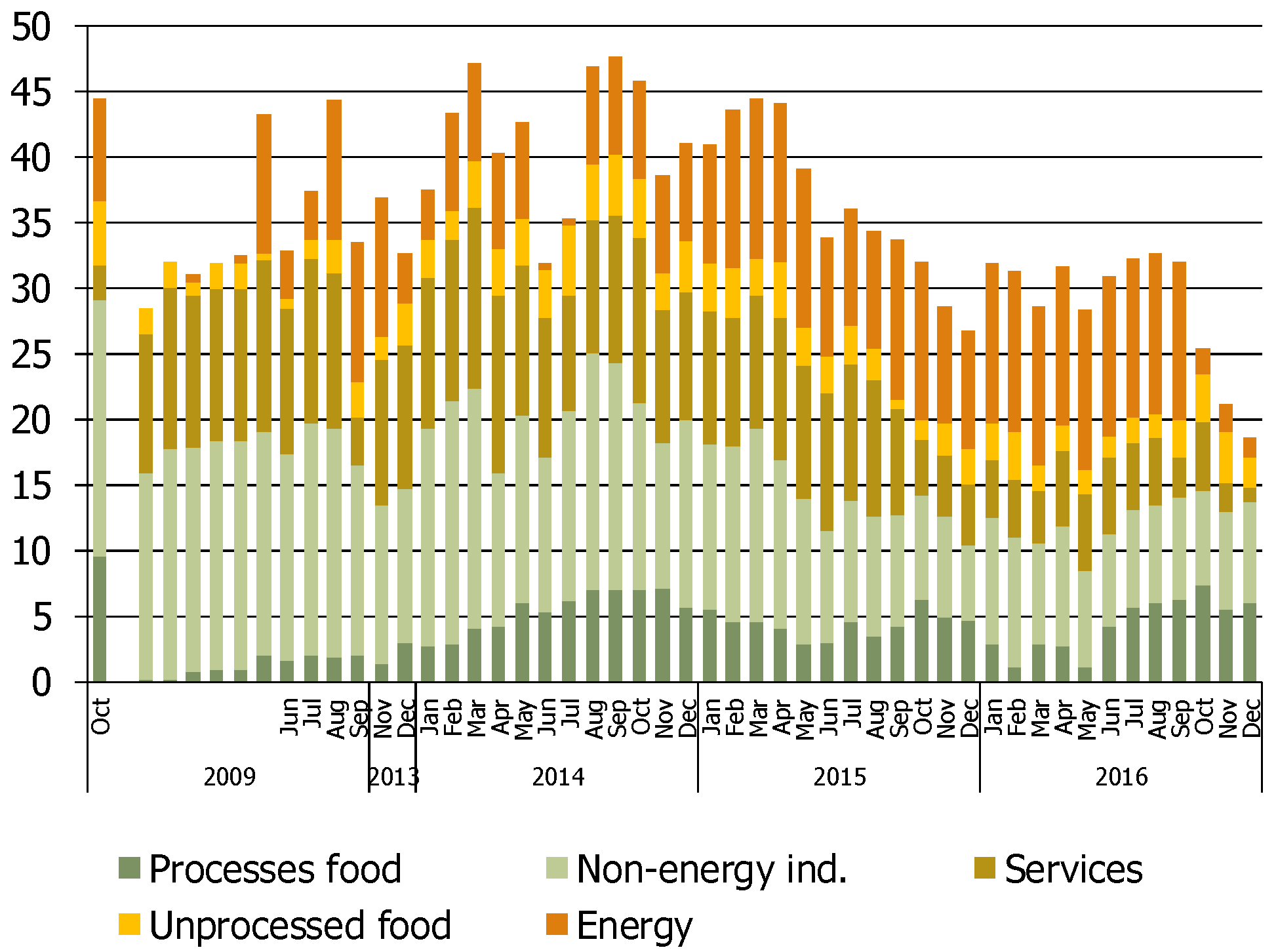
Another way of presenting this table could be by using colours to point out the items with negative and positive inflation rates. The BIAM provided this information in order to evaluate possible deflation situations. Thus, in a more schematic way, Figure 7 summarises this information by basic sub-aggregates, given in each case the weight of the basic components with negative inflation rates. The figure gives the information for all months in 2014–2016 and October 2009 as a reference month in middle of the economic crisis. It shows that the weight of basic components with negative inflation rates belonging to the Core was around 30% of the CPI in 2014 and the first half of 2015, because of important downward adjustments of prices in NEIG and also in SERV.

In the last few years, similar fully disaggregated results have been possible for a breakdown of the US CPI in 182 items, using the forecasting procedure proposed in Carlomagno and Espasa (2015a, 2015b). The format of this type of table can also be used to provide other information about the items, for instance, information on the relative unpredictability of the components as is done in Carlomagno (2016).

4. Evaluating Forecasting Performance

This section assesses BIAM real- time forecasting performance, first in absolute terms for the Euro Area, Spain and US and second in comparison with other Professional Forecasters available for the Euro Area.

Table 7. Forecasting performance in the Euro Area, Spain and US.

Monthly Forecasts	Sample Standard Deviation	MFE			RMSFE			Ratio RMSFE/Standard Deviation
		1	6	12	1	6	12	1	6	12
Euro Area
CPI	0.99	0.00	0.04	0.11	0.12	0.57	0.94	0.12	0.58	0.95
Core	0.56	− 0.01	−0.03	−0.07	0.10	0.29	0.52	0.18	0.52	0.93
Processed Food (PF)	1.45	−0.01	0.05	0.13	0.26	0.86	1.49	0.18	0.59	1.03
Non Energy Industrial Goods (NEIG)	0.42	0.00	−0.05	−0.12	0.19	0.34	0.54	0.45	0.81	1.29
Services (SER)	0.61	−0.02	−0.06	−0.12	0.15	0.31	0.51	0.25	0.51	0.84
Residual	4.09	0.05	0.52	1.10	0.65	2.56	3.81	0.16	0.63	0.93
Unprocessed Food (UPF)	2.11	0.00	0.17	0.26	0.66	1.60	2.34	0.31	0.76	1.11
Energy (EN)	6.60	0.13	0.94	1.92	1.01	4.32	6.14	0.15	0.65	0.93
Spain
CPI	1.59	−0.01	−0.04	−0.06	0.15	0.86	1.33	0.09	0.54	0.84
Core	1.11	−0.02	−0.12	−0.29	0.14	0.52	0.90	0.13	0.47	0.81
Processed Food (PF)	1.7	−0.02	0.05	0.06	0.34	1.18	1.96	0.20	0.69	1.15
Non Energy Industrial Goods (NEIG)	1.08	−0.01	−0.15	−0.37	0.25	0.63	0.95	0.23	0.58	0.88
Services (SER)	1.39	−0.04	−0.20	−0.43	0.17	0.54	0.91	0.12	0.39	0.66
Residual	5.22	0.02	0.37	1.05	0.60	3.23	4.51	0.11	0.62	0.86
Unprocessed Food (UPF)	2.88	0.03	0.04	−0.10	0.92	2.04	2.85	0.32	0.71	0.99
Energy (EN)	8.65	0.00	0.76	1.87	0.62	5.75	7.99	0.07	0.67	0.92
US
CPI	1.02	−0.01	−0.01	0.14	0.09	0.59	0.74	0.09	0.58	0.72
Core	0.29	0.00	0.01	0.03	0.08	0.26	0.33	0.27	0.88	1.14
Non Energy Commodities less Food	0.92	0.00	0.10	0.36	0.17	0.59	0.76	0.18	0.64	0.82
Durables	1.16	−0.02	0.18	0.59	0.22	0.97	1.08	0.19	0.84	0.93
Non Durables	0.85	0.02	0.03	0.13	0.23	0.53	0.81	0.28	0.62	0.95
Non Energy Services	0.42	0.00	−0.02	−0.09	0.07	0.22	0.32	0.17	0.52	0.75
Owner’s equivalent rent of primary res.	0.72	0.00	0.05	−0.18	0.06	0.29	0.37	0.09	0.41	0.52
Other Services	0.3	0.00	0.00	−0.03	0.11	0.28	0.42	0.37	0.92	1.40
Residual	4.52	−0.07	−0.08	0.51	0.25	2.14	2.93	0.06	0.47	0.65
Food	1.29	−0.02	−0.02	0.21	0.18	0.71	1.20	0.14	0.55	0.93
Energy	10.42	−0.14	−0.19	0.88	0.59	5.45	7.30	0.06	0.52	0.70

summarises the monthly forecasting performance of the y-o-y growth rate for 1, 6 and 12 months ahead of BIAM forecasts for the sample that goes from December 1999 to August 2016 for the headline CPI and for the main basic sub-aggregates for Euro Area and Spain and from January 2011 to December 2016 for US. Mean Forecast Errors (MFE) are shown in columns 3 to 5 and it can be seen how for headline CPI inflation the values that are close to zero. Looking at the components MFE only Energy (and therefore Residual inflation) at horizons 6 and 12 show some values that are apart from zero, but given the magnitude of the oscillations of this variable, we do not reject that it is zero. Regarding 12-months ahead forecasts, headline inflation showed a different behaviour before and after the crisis, which was reflected in greater positive MFEs in the first period that led to some bias concerns in one-year ahead forecasts. However, Bowles et al. (2007, 2010), pointed out that a large part of this systematic error can be explained by the sequence of asymmetric and largely unpredictable shocks that hit the Euro Area over the period and that when adjusting for these facts, there is far less evidence of a systematic underprediction or bias in the inflation expectations. Bowles et al. (2007) focused only on the Euro Area, but their results equally apply to Spain and US.

Columns 6 to 8 in Table 7 report on the Root Mean Squared Forecasting Error (RMSFE) of 1, 6 and 12 CPI forecasts for the Euro Area, Spain and the US. One- month ahead RMSFEs for Euro Area, Spain and US headline inflation are 0.12, 0.15 and 0.09 percentage points, respectively, and this uncertainty increases to 0.94, 1.33 and 0.74 p.p. at the 12-month horizon. Table 7 also reports on forecasts of all the basic sub-aggregates, showing the greatest unpredictability of Residual inflation versus Core inflation components at any horizon and also the biggest increase in unpredictability at longer horizons by Residual inflation components.

Provided that the forecasting models in the three areas are adequate, these RMSFE results can be interpreted in the sense that, by the proper nature of the phenomena, US inflation can be forecasted more accurately than Euro Area inflation, which also is more accurate than the Spanish CPI forecasts. However, to give additional evidence of the quality of the forecasting models used for the different models in the different areas, we compare the RMSFE values with the standard deviation of the corresponding in-sample values for the dependent variable, inflation. To this aim, column 2 in Table 7 reports these standard deviations during the sample estimation period for the CPI and all the basic sub-aggregates and Columns 9 to 11 provide the ratios between the corresponding out-of-sample RMSFEs and their in-sample standard deviation. If the forecasting models are appropriate and if we consider that Δ₁₂ log X_t is stationary, this ratio should be one or very close to one for a sufficiently long horizon. If the models are correct, longer horizons to reach a value of one reflect greater dependence on the past in the variable under question. Modelling the aggregate indirectly through the models of the components, it seems that we are capturing the long dynamic structure for the aggregate. It can be seen in Table 7 that the aforementioned ratios for headline inflation are less than one and that the greatest improvements over forecasting through the marginal mean are achieved in US. We can also say that the whole inflation forecasting modelling for Spanish data still provides this type of improvements at twelve periods ahead, and these improvements are greater than the corresponding improvements in the EA.

BIAM Forecast Comparison with ECB Survey of Professional Forecasters

The ECB Survey of Professional Forecasters (ECB-SPF) is a quarterly panel of forecasts, starting in 1999, surveying real GDP growth rate, HICP inflation and the unemployment rate expectations for the Euro Area as a whole. The panel covers institutions that are required to possess macroeconomic expertise relating to the Euro Area and not just to their own economy. In addition, they are required to have several years’ experience in forecasting and publishing forecasts. Respondents provide point forecasts for rolling horizons (one and two years ahead), fixed calendar year horizons (current year, next year and year after next) and longer-term expectations (five years ahead). They also provide the probability distributions that correspond to their point forecasts at all horizons. The BIAM has been providing real time forecasting results every month for the EA since its inception in January 1999, with a high participation rate of 91.4%. Therefore, while most research papers use benchmark models that are just random walk or AR specifications, the comparison with the forecasts obtained from ECB-SPF is more robust for comparing BIAM forecasts in two ways. First, because the combination of forecasts in general and consensus forecasts in particular, has been proved in the literature to produce more robust and more precise forecasts than individual forecasts, since the work by Bates and Granger (1969). In addition, because our consensus forecast is taken from the ECB Survey of Professional Forecasters, which includes the participation of more than 115 institutions since its implementation, and different econometric techniques, or even judgement, are applied. The ECB has conducted two specific surveys (Bowles et al. 2007 and ECB 2014) to ascertain the preferred type of model used by the participants to generate forecasts. Models vary according to the forecast horizon and to the variable being forecast. Most common methodologies for all horizons and variables, prominently to forecast inflation, are based on reduced form models, such as single equation, vector autoregressive (VAR) or vector error correction models (VECM). The participants also consider structural models, such as supply and demand-based macro models or dynamic stochastic general equilibrium (DSGE) models for longer forecast horizons.

There has been a large body of literature reporting success in forecasting with combinations of forecasts methods since the seminal work of Bates and Granger (1969). Later surveys on combinations of forecasts can be found in De Menezes et al. (2000), Clemen (1989), Newbold and Harvey (2002), Timmerman (2006) and, more recently, Wallis (2011) and Aiolfi et al. (2011), among others. It is also known that the simple average of point forecasts, dubbed as consensus, is usually a benchmark difficult to beat ((Stock and Watson 2004), called this fact the “forecast combination puzzle”). Regarding the ECB-SPF, recent papers like Genre et al. (2013), Conflitti et al. (2015) and Poncela and Senra (2017) have stated the relative good quality of the consensus forecasts against more sophisticated techniques.

Therefore, we are going to take the ECB-SPF consensus (defined as the average of the available forecasts at every moment in time) as a benchmark for comparison.

Table 8. Real-time inflation forecasting performance for the Euro Area.

Forecast Statistics and Time Span	1 Year Ahead		2 Years Ahead		Ratio BIAM/ ECB-SPF
Quarterly Forecasts	BIAM	ECB-SPF	BIAM	ECB-SPF	1 Year Ahead	2 Years Ahead
Mean Squared Forecast Error (MFE)
1999Q4–2016Q4	0.77	0.82	0.85	0.94	0.94	0.90
1999Q4–2007Q4	0.24	0.31	0.46	0.53	0.75	0.88
2008Q1–2016Q4	1.26	1.29	1.31	1.46	0.98	0.90
Root Mean Squared Forecast Error (RMSFE)
1999Q4–2016Q4	0.88	0.91	0.92	0.97	0.97	0.95
1999Q4–2007Q4	0.49	0.56	0.68	0.73	0.87	0.94
2008Q1–2016Q4	1.12	1.13	1.14	1.21	0.99	0.95
Mean Absolute Forecast Error (MAFE)
1999Q4–2016Q4	0.68	0.73	0.70	0.79	0.93	0.89
1999Q4–2007Q4	0.38	0.47	0.60	0.66	0.81	0.91
2008Q1–2016Q4	0.96	0.96	0.97	1.06	1.00	0.91

Source: ECB-SPF (http://www.ecb.europa.eu/stats/ecb_surveys/survey_of_professional_forecasters/html/index.en.html).

provides the main statistics for comparing one and two year forecast performance.

In the real-time forecasting period—1999 Q1 to 2016 Q4—the observed inflation was on average 1.77% with a standard deviation of 0.81 percentage points (p.p.). However, as Figure 5 shows, the sample behaved very differently. In the first part of the sample—1999 to 2007—mean inflation was 2.19% and in the second part—2008 to 2016—1.36%, and with different standard deviations. Thus, while in the first period the standard deviation was 0.28 p.p., it multiplied by 3.6 in the second part (1.01). This different behaviour persists also when looking at the forecasting performance, where there was also a large difference between pre and post- 2008. This is shown in Table 8 by the Root Mean Squared Forecast Error (RMSFE) and the Mean Absolute Forecasting Error (MAFE), which doubled pre-2008 values for both the BIAM and ECB-SPF forecasts. It must be said that the crisis per se, has not changed the BIAM disaggregation scheme, and the criteria collected in Table 1 still hold. Changes have occurred regarding inflation patterns, but not regarding the features pursued by the disaggregation. In the BIAM monthly forecasting exercise after the crisis, the disaggregation in operation was satisfactory.

The two last columns in Table 8 show the ratio of the alternative statistics between BIAM and ECB-SPF quarterly forecast errors. A smaller than one value of this ratio means an improvement of BIAM forecasts over ECB-SPF forecasts, and greater than 1 means the opposite. Diebold and Mariano (1995) tests (DM-tests) have been performed and the null of equal accuracy is not rejected by usual standards, although in one-year-ahead forecasts they are not too big. However this must not be seen as a demerit of BIAM forecasts. This is so, for several reasons. Above all, because BIAM forecasts provide much more information about inflation assessment and inflation forecasts in the EA than the consensus, and this turns out to be very informative for diagnosis. Therefore, even though the equal accuracy hypothesis is not rejected, the forecasts from the BIAM are much more useful. Second, although DM-tests are not significant, in all the periods analysed and with both absolute and squared forecast error loss functions, BIAM forecasts are always more accurate than ECB-SPF. Third, as previously explained, we are very ambitious when comparing BIAM forecasts with the ECB-SPF—instead of using, as most research papers do, benchmark models that are just random walks or AR specifications- which turns out to be a hard competitor and makes the comparison robust against a wide variety of models and procedures.

In the above paragraphs we have been using the Root Mean Square Forecast Error (RMSFE), when it is true that the generalized forecast error second moment matrix, Clements and Hendry (1993), allows for a better global forecasting accuracy measure for all forecast horizons, multiple disaggregation levels and for any linear scale-preserving transformation. However, this testing procedure of the forecasting accuracy between these two methods does not seem possible because in both cases the models used have been changing over time in different ways which have not been reported. Recall also the changing participation rates in the ECB-SPF. Besides, a joint evaluation of the BIAM system with respect to the Consensus in terms of multiple dimensions at the disaggregate level is not possible because the consensus does not provide disaggregated forecasts. Consequently, we have used the RMSFE as a way of appreciating in a sequence of many quarters which procedure has, in fact, been more accurate.

5. Conclusions

The methodology presented in the paper is focused on disaggregation. Its relevance relies on the fact that disaggregation gives an enlargement of the information set which allows for a better understanding of the aggregate. In addition, if the disaggregation is properly designed and implemented, it would provide an improvement in the forecast accuracy of the aggregate and would give results for a more precise diagnostic. The disaggregated schemes, to be useful as described above, must be designed to break down the aggregate in components by economic and institutional criteria. At the same time, they should be focused to end up with components with different statistical properties in trends, seasonal factors, breaks, persistence, etc., for which there are good data and with which valid econometric models could be built. These criteria do not determine a unique disaggregated formulation. What matters is that the disaggregation that one ends up with turns out to be useful, even when, depending on the characteristics of the data, it could be enlarged providing better results.

It must be noted that the results in the inflation literature comparing the performance of direct and indirect forecasting through the components might be misleading if they include papers which have not given adequate treatment to the aforementioned questions.

This disaggregation approach followed in the BIAM is denoted top-down and tends mainly to end up with components with different distributional properties, pointing out that the disaggregation structure is not necessarily given, but is something endogenous to the variable under study. In this sense, the disaggregation schemes applied to a given variable such as the CPI in several economies might be different. This is the case in the BIAM.

Another disaggregation approach could be based on finding intermediate sub-aggregates with important cross-restrictions between them –mainly common features, which should be exploited in the modelling processes. Successful applications of this approach are in Espasa et al. (2002a) and Espasa and Albacete (2007), where the authors used vector models for the basic sub-aggregates. For wider breakdowns as the BIAM’s experience suggests, Espasa and Mayo-Burgos (2013) and Carlomagno and Espasa (2015a, 2015b) propose a limited approach to find common features based on pairwise testing on the basic components. Then, groups of basic components with unique common trends or cycles can be formed, providing an intermediate disaggregation built in a bottom-up strategy. In this way, one can obtain an indirect forecast of the aggregate as well as forecasts for all the basic components. The last references mentioned include applications with good indirect forecasts for the headline inflation in different countries. Nevertheless, unless one is interested in forecasting the aggregate and all its components, the previous up-down approach for disaggregation followed in the BIAM is recommended.

The disaggregation applied in the BIAM is based on the sector attribute, but the geographical area could be another attribute on which the disaggregation could be focused. Studies such as Espasa et al. (2002a), Espasa and Albacete (2007) and Pino et al. (2016) show that the sector breakdown is more relevant than the regional one, and that a disaggregation based on both attributes offers only marginal advances over just disaggregating by sectors. For those reasons, the BIAM has implemented the sector approach. However, the results in Pino et al. (2016) show that if there is an interest in having forecasts for all sectors in all regions, their approach provides good results.

Another basic point in the BIAM methodology is the application of outlier corrections. With respect to the usual procedures that operate on the aggregate, the approach followed in the BIAM has the important advantage of being applied to the components. As shown in Carlomagno (2016), this strategy provides a better correction of the aggregate. In this approach, we correct the outlier in the specific components of the aggregate that require intervention. In the Euro Area, structural seasonal breaks have occurred because of changes in regulations by Eurostat. By modelling the components in the BIAM, we have been able to assign the appropriate seasonal change in the models for the indirect forecast of the headline inflation.

The BIAM assessment of inflation and inflation expectations is done by evaluating the new published data and making short and medium- term updated forecasts with corresponding fan charts. The evaluation of new data is done by means of forecasting errors at the component level. Then, it is possible to look for forecasting errors significantly different from zero in the components, even when the error in the aggregate is not. In any case, when working with disaggregates, a more precise correction is possible, and on many occasions, it is also very useful for diagnostic proposes.

In the paper, we have discussed some tables and plots used in the BIAM for reporting the forecasting results and the corresponding assessment. A one-page table which includes forecasting results for the aggregate and basic sub-aggregates for the remaining months of the current year and the months of the next two with confidence intervals turn out to be a simple and very useful device. The plot of the headline inflation with the contributions to it from the core and residual inflation values—alternatively with the contributions of the five basic sub-aggregates—is quite helpful for pointing out the sector or sectors which are contributing more to high or low headline inflation values. During periods of very low or negative values, a plot indicating the weight of the basic components with negative inflation rates in each basic sub-aggregate (see Figure 7) allows us to appreciate the weight of negative inflation rates in the components of the core and whether this weight is increasing or not. In that sense, plots reporting historical probabilities of having one-year ahead inflation rates (y-on-y) below a certain value, for instance, 1.5%, are also useful for evaluating deflations.

Another one-page table reporting headline forecasts for the annual inflation average of the current year and the next, jointly with the corresponding forecasts for all the basic components, signalling the values of the latter in relation to the confidence intervals of the former, is a simple instrument which provides a useful overall forecast for the different sectors of the economy.

This type of one-page table which gives information for the basic components could be used to report different characteristics of the basic components, such as unpredictability at different horizons.

Finally, we assess the real- time performance of the BIAM forecasts. We have checked that 1, 6 and 12-period forecasts from the BIAM have proven successful in reducing inflation unforecastability in absolute terms, both in Spain and the Euro Area. In the case of the Euro Area, we have shown the relative good performance in comparison with the real- time forecasts provided by the ECB-SPF, one and two years ahead.

References

1. Aiolfi, Marco, Carlos Capistran, and Allan Timmermann. 2011. Forecast combinations. In The Oxford Handbook of Economic Forecasting. Edited by Michael Clements and David Forbes Hendry. Oxford: Oxford University Press, pp. 355–88. [Google Scholar]
2. Altissimo, Filippo, Benoit Mojon, and Paolo Zaffaroni. 2007. Fast micro and slow macro: Can aggregation explain the persistence of inflation? Working Paper No. 2007-02. Federal Reserve of Chicago. [Google Scholar]
3. Aron, Janine, and John Muellbauer. 2012. Improving forecasting in an emerging economy, South Africa: Changing trends, long run restrictions and disaggregation. International Journal of Forecasting 28: 456–76. [Google Scholar] [CrossRef]
4. Athanasopoulos, George, Roman Ahmed, and Rob J. Hyndman. 2009. Hierarchical forecasts for Australian domestic tourism. International Journal of Forecasting 25: 146–66. [Google Scholar] [CrossRef]
5. Bates, John M., and Clive W. J. Granger. 1969. The combination of forecasts. Operational Research Quarterly 20: 451–68. [Google Scholar] [CrossRef]
6. Beck, Guenter W., Kirstin Hubrich, and Massimiliano Marcellino. 2011. On the Importance of Sectoral and Regional Shocks for Price-Setting. Working Paper Series 1334, Frankfurt, Germany: European Central Bank. [Google Scholar]
7. BIAM 266. 2016. Bulletin of EU&US Inflation and Macroeconomic Analysis. Madrid: Universidad Carlos III de Madrid, Available online: http://www.uc3m.es/biam (accessed on 30 December 2016).
8. Bils, Mark, and Peter J. Klenow. 2004. Some evidence on the importance of sticky prices. Journal of Political Economy 112: 947–85. [Google Scholar] [CrossRef]
9. Boivin, Jean, Marc P. Giannoni, and Ilian Mihov. 2009. Sticky prices and monetary policy: Evidence from disaggregated us data. The American Economic Review 99: 350–84. [Google Scholar] [CrossRef]
10. Bowles Carlos, Roberta Fritz, Véronique Genre, Geoff Kenny, Aidan Meyler, and Tuomas Rautanen. 2007. The ECB Survey of Professional Forecasters (SPF). A Review after Eight Years’ Experience. (Occasional Paper Series 59); Frankfurt, Germany: European Central Bank. [Google Scholar]
11. Bowles, Carlos, Roberta Fritz, Véronique Genre, Geoff Kenny, Aidan Mayler, and Tuomas Rautanen. 2010. An Evaluation of the Growth and Unemployment Forecasts in the ECB Survey of Professional Forecasters. OECD Journal: Journal of Business Cycle Measurement and Analysis 2: 63–90. [Google Scholar] [CrossRef]
12. Britton, Erik, Paul G. Fisher, and John D. Whitley. 1998. The Inflation Report projections: understanding the fan chart. Bank of England Quarterly Bulletin 38: 30–37. [Google Scholar]
13. Carlomagno, Guillermo. 2016. Discovering Common Features in a Large Set of Disaggregates. Methodology, Modelling and Forecasting. Ph.D. dissertation, Statistics Department, Universidad Carlos III, Madrid, Spain, February. [Google Scholar]
14. Carlomagno, Guillermo, and Antoni Espasa. 2015a. Discovering Common Trends in a Large Set of Disaggregates: Statistical Procedures and Their Properties. UC3M Working Paper 15-19. Madrid: University Carlos III. [Google Scholar]
15. Carlomagno, Guillermo, and Antoi Espasa. 2015b. Forecasting a Large Set of Disaggregates with Common Trends and Outliers. UC3M Working Paper 15-18. Madrid: University Carlos III. [Google Scholar]
16. Castle, Jennifer L., Jurgen A. Doornik, David F. Hendry, and Felix Pretis. 2015. Detecting location shifts during model selection by step-indicator saturation. Econometrics 3: 240–64. [Google Scholar] [CrossRef]
17. Clark, Todd E. 2006. Disaggregate evidence on the persistence of consumer price inflation. Journal of Applied Econometrics 21: 563–87. [Google Scholar] [CrossRef]
18. Clemen, Robert T. 1989. Combining forecasts: A review and annotated bibliography. International Journal of Forecasting 5: 559–83. [Google Scholar] [CrossRef]
19. Clements, Michael P., and David F. Hendry. 1993. On the limitations of comparing mean squared forecast errors. Journal of Forecasting 12: 617–37, (With Discussion 669–76). [Google Scholar] [CrossRef]
20. Conflitti, Cristina, Christine De Mol, and Domenico Giannone. 2015. Optimal combination of survey forecasts. International Journal of Forecasting 31: 1096–103. [Google Scholar] [CrossRef]
21. Cuevas, Angel, Enrique Quilis, and Antoni Espasa. 2015. Quarterly Regional GDP Flash Estimates by Means of Benchmarking and Chain-Linking. Journal of Official Statistics 31: 627–47. [Google Scholar] [CrossRef]
22. De Menezes, Lillian M., Derek W. Bunn, and James W. Taylor. 2000. Review of guidelines for the use of combined forecasts. European Journal of Operational Research 120: 190–204. [Google Scholar] [CrossRef]
23. Diebold, Francis X., and Roberto S. Mariano. 1995. Comparing predictive accuracy. Journal of Business & Economic Statistics 20: 134–44. [Google Scholar]
24. Doornik, Jurgen A., and David F. Hendry. 2016. Outliers and models selection: Discussion of the paper by Soren Johansen and Bent Nielsen. Scandinavian Journal of Statistics 43: 360–65. [Google Scholar] [CrossRef]
25. Dreger, Christian, and Massimiliano Marcellino. 2007. A Macroeconometric Model for the Euro economy. Journal of Policy Modeling 29: 1–13. [Google Scholar] [CrossRef]
26. Dreger, Christian. 2002. A Macroeconometric Model for the Euro Area. Halle (IWH), Germany: Institute for Economic Research, manuscript. [Google Scholar]
27. ECB. 2014. Fifteen years of the ECB Survey of Professional Forecasters. In ECB Monthly Bulletin. Frankfurt: European Central Bank. [Google Scholar]
28. EFN. 2013. EFN Report Economic Outlook for the Euro Area in 2013 and 2014. Available online: http://www.eui.eu/Documents/RSCAS/Research/EFN/Reports/EFN2013/EFN2013autumn.pdf (accessed on 30 September 2017).
29. Espasa, Antoni, and Rebeca Albacete. 2007. Econometric modelling for short-term inflation forecasting in the euro area. Journal of Forecasting 26: 303–16. [Google Scholar] [CrossRef] [Green Version]
30. Espasa, Antoni, and M. Llanos Matea. 1991. Underlying Inflation in the Spanish Economy: Estimation and Methodology. Working Paper 91-30. Madrid, Spain: Department of Economics, Universidad Carlos III, November, Italian translation published in Note Economiche. vol. XXI, No. 3, 477–93. [Google Scholar]
31. Espasa, Antoni, and Iván Mayo-Burgos. 2013. Forecasting aggregates and disaggregates with common features. International Journal of Forecasting 29: 718–32. [Google Scholar] [CrossRef] [Green Version]
32. Espasa, Antoni, Ascensión Molina, and Eva Ortega. 1984. Forecasting the Rate of Inflation by Means of the Consumer Price Index. Working paper 8416. Paper presented at the Fourth International Symposium on Forecasting, London, UK; Banco de España, Madrid, Spain. [Google Scholar]
33. Espasa, Antoni, M. Llanos Matea, and M. Cruz Manzano. 1987. La inflación subyacente en la economía española: Estimación y metodología. In Boletín Económico. Madrid: Banco de España. [Google Scholar]
34. Espasa, Antoni, Eva Senra, and Rebeca Albacete. 2002a. Forecasting inflation in the European Monetary Union: A disaggregated approach by countries and by sectors. The European Journal of Finance 8: 402–21. [Google Scholar] [CrossRef]
35. Espasa, Antoni, Pilar Poncela, and Eva Senra. 2002. Forecasting Monthly US Consumer Price Indexes through a Disaggregated I (2) Analysis. Working Paper 02-03. Madrid: University Carlos III. [Google Scholar]
36. Genre Véronique, Geoff Kenny, Aida Meyler, and Allan Timmermann. 2013. Combining expert forecasts: Can anything beat the simple average? International Journal of Forecasting 29: 108–21. [Google Scholar] [CrossRef]
37. Hendry, David F. 2006. Robustifying forecasts from equilibrium-correction systems. Journal of Econometrics 135: 399–426. [Google Scholar] [CrossRef]
38. Hendry, David. F., and Jurgen A. Doornik. 2014. Empirical Model Discovery and Theory Evaluation. Cambridge: MIT Press. [Google Scholar]
39. Hendry, David F., and Kirstin Hubrich. 2011. Combining disaggregate forecasts or combining disaggregate information to forecast an aggregate. Journal of Business & Economic Statistics 29: 216–27. [Google Scholar]
40. Hyndman, Rob J., Roman Ahmed, George Athanasopoulos, and Han Lin Shang. 2011. Optimal combination forecasts for hierarchical time series. Computational Statistics & Data Analysis 55: 2579–89. [Google Scholar]
41. Imbs, Jean, Haroon Mumtaz, Morten O. Ravn, and Helene Rey. 2005. PPP strikes back: Aggregation and the real exchange rate. The Quarterly Journal of Economics 120: 1–43. [Google Scholar]
42. Johansen, Soren, and Bent Nielsen. 2016. Asymptotic theory of outlier detection algorithms for linear time series regression models. Scandinavian Journal of Statistics 43: 321–48. [Google Scholar] [CrossRef]
43. Juselius, Katarina. 2015. Haavelmo’s probability approach and the cointegrated VAR. Econometric Theory 31: 213–32. [Google Scholar] [CrossRef]
44. Lorenzo, Fernando. 1997. Modelización de la Inflación con fines de Predicción y Diagnóstico. Ph.D. dissertation, Department of Statistics and Econometrics, Universidad Carlos III, Madrid, Spain, September. [Google Scholar]
45. Lunnemann, Patrick, and Thomas Y. Mathä. 2004. How persistent is disaggregate inflation? An analysis across EU 15 countries and HICP sub-indices. ECB Working Paper 415. Frankfurt, Germany: European Central Bank. [Google Scholar]
46. Lütkepohl, Helmut. 1987. Forecasting Aggregated Vector ARMA Processes. Berlin: Springer-Verlag. [Google Scholar]
47. Minguez, Román, and Antoni Espasa. 2006. A Time Series Disaggregated Model to Forecast GDP in the Eurozone. In Growth and Cycle in the Eurozone. Edited by Gian Luigi Mazzi and Giovanni Savio. Basingstoke: Palgrave, chp. 17. pp. 213–20. [Google Scholar]
48. Newbold, Paul, and David I. Harvey. 2002. Forecast combination and encompassing. In A Companion to Economic Forecasting. Edited by Michael P. Clements and David F. Hendry. Hoboken: Wiley, pp. 268–83. [Google Scholar]
49. Osborn, Denise, and Michael P. Clements. 2002. Unit root versus deterministic representations of seasonality for forecasting. In A Companion to Economic Forecasting. Edited by Michael P. Clements and David F. Hendry. Malden: Blackwell Publishers. [Google Scholar]
50. Osborn, Denise, Saeed Heravi, and Chris R. Birchenhall. 1999. Seasonal unit roots and forecasts of two-digit European industrial production. International Journal of Forecasting 15: 27–47. [Google Scholar] [CrossRef]
51. Peach, Richard W., Robert Rich, and Alexis Antonaides. 2004. The historical and recent behaviour of goods and services inflation. FRBNY Economic Policy Review 10: 19–31. [Google Scholar]
52. Peach, Richard W., Robert Rich, and M. Hendry Linder. 2013. The parts are more than the whole: separating goods and services to predict core inflation. Current Issues in Economic and Finance 19: 1–8. [Google Scholar]
53. Pino, Gabriel, Juan de Dios Tena, and Antoni Espasa. 2016. Geographical disaggregation of sectoral inflation. Econometric modelling of the Euro area and Spanish economies. Applied Economics 48: 799–815. [Google Scholar] [CrossRef]
54. Poncela, Pilar, and Eva Senra. 2017. Measuring uncertainty and assessing its predictive power in the euro area. Empirical Economics 53: 165–82. [Google Scholar] [CrossRef]
55. Stock, James H., and Mark W. Watson. 2004. Combination forecasts of output growth in a seven-country data set. Journal of Forecasting 23: 405–30. [Google Scholar] [CrossRef]
56. Timmermann, Allan. 2006. Forecast combinations. In Handbook of Economic Forecasting. Edited by Graham Elliott, Clive Granger and Allan Timmermann. Amsterdam: Elsevier, vol. 1, pp. 135–96. [Google Scholar]
57. Wallis, Kenneth F. 1999. Asymmetric density forecasts of inflation and the Bank of England’s fan chart. National Institute Economic Review 167: 106–12. [Google Scholar] [CrossRef]
58. Wallis, Kenneth F. 2011. Combining forecasts—Forty years later. Applied Financial Economics 21: 33–41. [Google Scholar] [CrossRef]
1
In general, this assignment is approximated because some basic components might include prices corresponding to two different basic sub-aggregates, for instance, NEIG and SERV. Nevertheless, when this is the case, the prices inside the basic component belong mostly to one basic sub-aggregate.
2
We are grateful to Ángel Sánchez for preparing this figure.
Figure 1. Basic disaggregation for Euro Area HICP and Spain and US CPI. Source: Eurostat, INE and Federal Reserve.
Econometrics 05 00044 g001
Figure 2. US CPI breakdown.
Econometrics 05 00044 g002
Figure 3. Δ12log (US CPI) and its 164 components). Source: Carlomagno (2016).
Econometrics 05 00044 g003
Figure 4. Year-on year Euro Area inflation rate and contributions of main components. Source: Eurostat & BIAM (UC3M). Date: 18 January 2017.
Econometrics 05 00044 g004
Figure 5. Euro Area inflation forecasts and uncertainty surrounding the forecasts (year-on-year rates). Source: Eurostat & BIAM (UC3M). Date: 18 January 2017.
Econometrics 05 00044 g005
Figure 6. Probability of the year- on- year Euro Area HICP to be under 1% and 1.5% after the month of reference. Source: INE & BIAM (UC3M). Date: 24 November 2016.
Econometrics 05 00044 g006
Figure 7. COICOP Spanish subclasses with negative y-o-y inflation rates. Source: INE & BIAM (UC3M). Date: 13 January 2017.
Econometrics 05 00044 g007