Cointegration between Trends and Their Estimators in State Space Models and Cointegrated Vector Autoregressive Models

Abstract

A state space model with an unobserved multivariate random walk and a linear observation equation is studied. The purpose is to find out when the extracted trend cointegrates with its estimator, in the sense that a linear combination is asymptotically stationary. It is found that this result holds for the linear combination of the trend that appears in the observation equation. If identifying restrictions are imposed on either the trend or its coefficients in the linear observation equation, it is shown that there is cointegration between the identified trend and its estimator, if and only if the estimators of the coefficients in the observation equations are consistent at a faster rate than the square root of sample size. The same results are found if the observations from the state space model are analysed using a cointegrated vector autoregressive model. The findings are illustrated by a small simulation study.

1. Introduction and Summary

This paper is inspired by a study on long-run causality, see Hoover et al. (2014). Causality is usually studied for a sequence of multivariate i.i.d. variables using conditional independence, see Spirtes et al. (2000) or Pearl (2009). For stationary autoregressive processes, causality is discussed in terms of the variance of the shocks, that is, the variance of the i.i.d. error term. For nonstationary cointegrated variables, the common trends play an important role for long-run causality. In Hoover et al. (2014), the concept is formulated in terms of independent common trends and their causal impact coefficients on the nonstationary observations. Thus, the emphasis is on independent trends, and how they enter the observation equations, rather than on the variance of the measurement errors.

The trend is modelled as an $m-$dimensional Gaussian random walk, starting at $T_0$,

$$T_{t+1}=T_t+{\eta }_{t+1},t=0,\dots ,n-1,$$

(1)

where ${\eta }_t$ are i.i.d. $N_m(0,{\mathrm{\Omega }}_{\eta })$, that is, Gaussian in m dimensions with mean zero and $m\times m$ variance ${\mathrm{\Omega }}_{\eta }>0$. This trend has an impact on future values of the $p-$dimensional observation $y_t$ modelled by

$$y_{t+1}=B{T}_t+{\epsilon }_{t+1},t=0,\dots ,n-1,$$

(2)

where ${\epsilon }_t$ are i.i.d. $N_p(0,{\mathrm{\Omega }}_{\epsilon })$ and ${\mathrm{\Omega }}_{\epsilon }>0$. It is also assumed that the ${\epsilon }_s$ and ${\eta }_t$ are independent for all s and t. In the following the joint distribution of $T_1,\dots ,T_n,y_1,\dots ,y_n$ conditional on a given value of $T_0$ is considered.

The observations are collected in the matrices $Y_n$, $p\times n$, and $\Delta Y_n$, $p\times (n-1)$, which are defined as

$$Y_n=(y_1,\dots ,y_n),\mathrm{and}\Delta Y_n=(y_2-y_1,\dots ,y_n-y_{n-1}).$$

The processes $y_t$ and $T_t$ are obviously nonstationary, but the conditional distribution of $Y_n$ given $T_0$ is well defined. We define

$$\begin{array}{cc}\hfill E_t{T}_t& =E(T_t|Y_t,T_0),\hfill \\ \hfill V_t& =Va{r}_t(T_t)=Var(T_t|Y_t,T_0).\hfill \end{array}$$

Then the density of $Y_n$ conditional on $T_0$ is given by the prediction error decomposition

$$p(Y_n|T_0)=p(y_1|T_0)\prod _{t=1}^{n-1}p(y_{t+1}|Y_t,T_0),$$

where $y_{t+1}$ given $(Y_t,T_0)$ is p dimensional Gaussian with mean and variance

$$\begin{array}{cc}\hfill E_t{y}_{t+1}& =B{E}_t{T}_t,\hfill \\ \hfill Va{r}_t(y_{t+1})& =B{V}_t{B}^{\prime }+{\mathrm{\Omega }}_{\epsilon }.\hfill \end{array}$$

In this model it is clear that $y_t$ and $T_t$ cointegrate, that is, $y_{t+1}-B{T}_{t+1}={\epsilon }_{t+1}-B{\eta }_{t+1}$ is stationary, and the same holds for $T_t$ and the extracted trend $E_t{T}_t=E(T_t|y_1,\dots ,y_t,T_0)$. Note that in the statistical model defined by (1) and (2) with parameters $B,{\mathrm{\Omega }}_{\eta }$, and ${\mathrm{\Omega }}_{\epsilon }$, only the matrices $B{\mathrm{\Omega }}_{\eta }{B}^{\prime }$ and ${\mathrm{\Omega }}_{\epsilon }$ are identified because for any $m\times m$ matrix $\xi$ of full rank, $B{\xi }^{-1}$ and $\xi {\mathrm{\Omega }}_{\eta }{\xi }^{\prime }$ give the same likelihood, by redefining the trend as $\xi T_t$.

Let ${\widehat{E}}_t{T}_t$ be an estimator of $E_t{T}_t$. The paper investigates whether there is cointegration between $E_t{T}_t$ and ${\widehat{E}}_t{T}_t$ given two different estimation methods: A simple cointegrating regression and the maximum likelihood estimator in an autoregressive representation of the state space model.

Section 2, on the probability analysis of the data generating process, formulates the model as a common trend state space model, and summarizes some results in three Lemmas. Lemma 1 contains the Kalman filter equations and the convergence of $Var(T_t|y_1,\dots ,y_t,T_0)$, see Durbin and Koopman (2012), and shows how its limit can be calculated by solving an eigenvalue problem. Lemma 1 also shows how $y_t$ can be represented in terms of its prediction errors $v_j=y_j-E_{j-1}{y}_j$, $j=1,\dots ,t$. This result is used in Lemma 2 to represent $y_t$ in steady state as an infinite order cointegrated vector autoregressive model, see (Harvey 2006, p. 373). Section 3 discusses the statistical analysis of the data and the identification of the trends and their loadings. Two examples are discussed. In the first example, only B is restricted and the trends are allowed to be correlated. In the second example, B is restricted but the trends are uncorrelated, so that also the variance matrix is restricted. Lemma 3 analyses the data from (1) and (2) using a simple cointegrating regression, see Harvey and Koopman (1997), and shows that the estimator of the coefficient B suitably normalized is n-consistent.

Section 4 shows in Theorem 1 that the spread between $B{E}_t{T}_t$ and its estimator $\widehat{B}{\widehat{E}}_t{T}_t$ is asymptotically stationary irrespective of the identification of B and $T_t$. Then Theorem 2 shows that the spread between $E_t{T}_t$ and its estimator ${\widehat{E}}_t{T}_t$ is asymptotically stationary if and only if B has been identified so that the estimator of B is superconsistent, that is, consistent at a rate faster than $n^{1/2}$.

The findings are illustrated with a small simulation study in Section 5. Data are generated from (1) and (2) with $T_0=0$, and the observations are analysed using the cointegrating regression discussed in Lemma 3. If the trends and their coefficients are identified by the trends being independent, the trend extracted by the state space model does not cointegrate with its estimator. If, however, the trends are identified by restrictions on the coefficients alone, they do cointegrate.

2. Probability Analysis of the Data Generating Model

This section contains first two examples, which illustrate the problem to be solved. Then a special parametrization of the common trends model is defined and some, mostly known, results are given in Lemmas 1 concerning the Kalman filter recursions. Lemma 2 is about the representation of the steady state solution as an autoregressive process. All proofs are given in the Appendix.

2.1. Two Examples

Two examples are given which illustrate the problem investigated. The examples are analysed further by a simulation study in Section 5.

Example 1.

In the first example the two random walks $T_{1t}$ and $T_{2t}$ are allowed to be dependent, so ${\mathrm{\Omega }}_{\eta }$ is unrestricted, and identifying restrictions are imposed only on their coefficients B. The equations are

$$\begin{array}{ccc}\hfill y_{1,t+1}& =& T_{1t}+{\epsilon }_{1,t+1},\hfill \\ \hfill y_{2,t+1}& =& T_{2t}+{\epsilon }_{2,t+1},\hfill \\ \hfill y_{3,t+1}& =& b_{31}{T}_{1t}+b_{32}{T}_{2t}+{\epsilon }_{3,t+1}.\hfill \end{array}$$

(3)

for $t=0,\dots ,n-1$.Thus, $y_t={(y_{1t},y_{2t},y_{3t})}^{\prime }$, $T_t={(T_{1t},T_{2t})}^{\prime }$, and

$$B=\left(\begin{array}{cc}1& 0\\ 0& 1\\ b_{31}& b_{32}\end{array}\right).$$

(4)

Moreover, ${\mathrm{\Omega }}_{\eta }>0$ is $2\times 2$, ${\mathrm{\Omega }}_{\epsilon }>0$ is $3\times 3$, and both are unrestricted positive definite. Simulations indicate that $E_t{y}_{t+1}-{\widehat{E}}_t{y}_{t+1}=B{E}_t{T}_t-\widehat{B}{\widehat{E}}_t{T}_t$ is stationary, and this obviously implies that the same holds for the first two coordinates $E_t{T}_{1t}-{\widehat{E}}_t{T}_{1t}$ and $E_t{T}_{2t}-{\widehat{E}}_t{T}_{2t}$.      ■

Example 2.

The second example concerns two independent random walks $T_{1t}$ and $T_{2t}$, and the three observation equations

$$\begin{array}{ccc}\hfill y_{1,t+1}& =& T_{1t}+{\epsilon }_{1,t+1},\hfill \\ \hfill y_{2,t+1}& =& b_{21}{T}_{1t}+T_{2t}+{\epsilon }_{2,t+1},\hfill \\ \hfill y_{3,t+1}& =& b_{31}{T}_{1t}+b_{32}{T}_{2t}+{\epsilon }_{3,t+1}.\hfill \end{array}$$

(5)

In this example

$$B=\left(\begin{array}{cc}1& 0\\ b_{21}& 1\\ b_{31}& b_{32}\end{array}\right),{\mathrm{\Omega }}_{\eta }=diag({\sigma }_1^2,{\sigma }_2^2),$$

(6)

and ${\mathrm{\Omega }}_{\epsilon }>0$ is $3\times 3$ and unrestricted positive definite. Thus the nonstationarity is caused by two independent trends. The first, $T_{1t}$, is the cause of the nonstationarity of $y_{1t}$, whereas both trends are causes of the nonstationarity of $(y_{2t},y_{3t})$. From the first equation it is seen that $y_{1t}$ and $T_{1t}$ cointegrate. It is to be expected that also the extracted trend $E_t{T}_{1t}$ cointegrates with $T_{1t}$, and also that $E_t{T}_{1t}$ cointegrates with its estimator ${\widehat{E}}_t{T}_{1t}$. This is all supported by the simulations. Similarly, it turns out that

$$E_t{y}_{2,t+1}-{\widehat{E}}_t{y}_{2,t+1}=b_{21}{E}_t{T}_{1t}-{\widehat{b}}_{21}{\widehat{E}}_t{T}_{1t}+E_t{T}_{2t}-{\widehat{E}}_t{T}_{2t},$$

is asymptotically stationary. In this case, however, $E_t{T}_{2t}-{\widehat{E}}_t{T}_{2t}$ is not asymptotically stationary, and the paper provides an answer to why this is the case.      ■

The problem to be solved is why in the first example cointegration was found between the extracted trends and their estimators, and in the second example they do not cointegrate. The solution to the problem is that it depends on the way the trends and their coefficients are identified. For some identification schemes the estimator of B is n-consistent, and then stationarity of $E_t{T}_t-{\widehat{E}}_t{T}_t$ can be proved. But if identification is achieved by imposing restrictions also on the covariance of the trends, as in Example 2, then the estimator for B is only $n^{1/2}$-consistent, and that is not enough to get asymptotic stationarity of $E_t{T}_t-{\widehat{E}}_t{T}_t$.

2.2. Formulation of the Model as a Common Trend State Space Model

The common trend state space model with constant coefficients is defined by

$$\begin{array}{c}{\alpha }_{t+1}={\alpha }_t+{\eta }_t,\\ y_t=B{\alpha }_t+{\epsilon }_t,\end{array}$$

(7)

$t=1,\dots ,n$, see Durbin and Koopman (2012) or Harvey (1989), with initial state ${\alpha }_1$. Here ${\alpha }_t$ is the unobserved m−dimensional state variable and $y_t$ the p−dimensional observation and B is $p\times m$ of rank $m<p$. The errors ${\epsilon }_t$ and ${\eta }_t$ are as specified in the discussion of the model given by (1) and (2).

Defining $T_t={\alpha }_{t+1},t=0,\dots ,n$, gives the model (1) and (2). Note that in this notation $E_t{T}_t=E_t{\alpha }_{t+1}$ is the predicted value of the trend ${\alpha }_{t+1}$, which means that it is easy to formulate the Kalman filter.

The Kalman filter calculates the prediction $a_{t+1}=E_t{\alpha }_{t+1}$ and its conditional variance $P_{t+1}=Va{r}_t({\alpha }_{t+1})$ by the equations

$$\begin{array}{cc}\hfill a_{t+1}& =a_t+P_t{B}^{\prime }{(B{P}_t{B}^{\prime }+{\mathrm{\Omega }}_{\epsilon })}^{-1}(y_t-E_{t-1}(y_t)),\hfill \end{array}$$

(8)

$$\begin{array}{cc}\hfill P_{t+1}& =P_t+{\mathrm{\Omega }}_{\eta }-P_t{B}^{\prime }{(B{P}_t{B}^{\prime }+{\mathrm{\Omega }}_{\epsilon })}^{-1}B{P}_t,\hfill \end{array}$$

(9)

starting with $a_1={\alpha }_1$ and $P_1=0$.

The recursions (8) and (9) become

$$\begin{array}{cc}\hfill E_{t+1}{T}_{t+1}& =E_t{T}_t+K_t^{\prime }(y_{t+1}-E_t{y}_{t+1}),\hfill \end{array}$$

(10)

$$\begin{array}{cc}\hfill V_{t+1}& ={\mathrm{\Omega }}_{\eta }+V_t-K_t^{\prime }B{V}_t,\hfill \end{array}$$

(11)

$t=0,\dots ,n-1$ starting with $E_1{T}_1=T_0$ and $V_1={\mathrm{\Omega }}_{\eta }$, and defining the Kalman gain

$$K_t^{\prime }=V_t{B}^{\prime }{(B{V}_t{B}^{\prime }+{\mathrm{\Omega }}_{\epsilon })}^{-1}.$$

(12)

Lemma 1 contains the result that $V_{t+1}$ converges for $t\to \infty$ to a finite limit V, which can be calculated by solving an eigenvalue problem. Equation (11) is an algebraic Ricatti equation, see Chan et al. (1984), where the convergence result can be found. The recursion (10) is used to represent $y_{t+1}$ in terms of its cumulated prediction errors $v_{t+1}=y_{t+1}-E_t{y}_{t+1}$, as noted by Harvey (2006, Section 7.3.2).

Lemma 1.

Let $V_t=Var(T_t|Y_t)$ and $E_t{T}_t=E(T_t|Y_t)$.

(a) The recursion for $V_t$, (11), can be expressed as

$$V_{t+1}={\mathrm{\Omega }}_{\eta }+V_t-V_t{(V_t+{\mathrm{\Omega }}_B)}^{-1}{V}_t\to V,t\to \infty ,$$

(13)

where ${\mathrm{\Omega }}_B=Var({\overline{B}}^{\prime }{\epsilon }_t|B_{\perp }^{\prime }{\epsilon }_t)$ for $\overline{B}=B{(B^{\prime }B)}^{-1}$. Moreover,

$$I_m-K_t^{\prime }B=I_m-V_t{B}^{\prime }{(B{V}_t{B}^{\prime }+{\mathrm{\Omega }}_{\epsilon })}^{-1}B\to I_m-K^{\prime }B={\mathrm{\Omega }}_B{(V+{\mathrm{\Omega }}_B)}^{-1},t\to \infty ,$$

(14)

which has positive eigenvalues less than one, such that $I_m-K^{\prime }B$ is a contraction, that is, ${(I_m-K^{\prime }B)}^n\to 0$, $n\to \infty$.

(b) The limit of $V_t$ can be found by solving the eigenvalue problem

$$|\lambda {\mathrm{\Omega }}_B-{\mathrm{\Omega }}_{\eta }|=0,$$

for eigenvectors W and eigenvalues $({\lambda }_1,\dots ,{\lambda }_m)$, such that $W^{\prime }{\mathrm{\Omega }}_{B}W=I_m$ and $W^{\prime }{\mathrm{\Omega }}_{\eta }W=diag({\lambda }_1,\dots ,{\lambda }_m)$. Hence, $W^{\prime }VW=diag({\tau }_1,\dots ,{\tau }_m)$ for

$${\tau }_i=\frac{1}{2}\{{\lambda }_i+{({\lambda }_i^2+4{\lambda }_i)}^{1/2}\}.$$

(15)

(c) Finally, using the prediction error, $v_{t+1}=y_{t+1}-E_t{y}_{t+1}$, it is found from (10) that

$$E_t{T}_t=T_0+\sum _{j=1}^t{K}_{j-1}^{\prime }{v}_j,and{y}_{t+1}=v_{t+1}+B(T_0+\sum _{j=1}^t{K}_{j-1}^{\prime }{v}_j).$$

(16)

The prediction errors are independent Gaussian with mean zero and variances

$$Var(v_{t+1})=Va{r}_t(y_{t+1})=Va{r}_t(B{T}_t+{\epsilon }_{t+1})=B{V}_t{B}^{\prime }+{\mathrm{\Omega }}_{\epsilon }\to BV{B}^{\prime }+{\mathrm{\Omega }}_{\epsilon },t\to \infty ,$$

such that in steady state the prediction errors are i.i.d. $N_p(0,BV{B}^{\prime }+{\mathrm{\Omega }}_{\epsilon })$, and (16) shows that $y_t$ is approximately an $AR(\infty )$ process, for which the reduced form autoregressive representation can be found, see (Harvey 2006, Section 7.3.2).

Lemma 2.

If the system (7) is in steady state, prediction errors $v_t$ are i.i.d. $N(0,BV{B}^{\prime }+{\mathrm{\Omega }}_{\epsilon })$ and

$$\Delta y_t=\Delta v_t+B{K}^{\prime }{v}_{t-1}.$$

(17)

Applying the Granger Representation Theorem, $y_t$ is given by

$$\Delta y_t=\alpha {\beta }^{\prime }{y}_{t-1}+\sum _{i=1}^{\infty }{\mathrm{\Gamma }}_i\Delta y_{t-i}+v_t.$$

(18)

Here $\alpha =-K_{\perp }{(B_{\perp }^{\prime }{K}_{\perp })}^{-1}$ and $\beta =B_{\perp }$.

2.3. Cointegration among the Observations and Trends

In model (1) and (2), the equation $y_{t+1}=B{T}_t+{\epsilon }_{t+1}$ shows that $y_t$ and $T_t$ are cointegrated. It also holds that $T_t-E_t{T}_t$ is asymptotically stationary because

$$v_{t+1}=y_{t+1}-E_t{y}_{t+1}=B{T}_t+{\epsilon }_{t+1}-B{E}_t{T}_t,$$

which shows that $B(T_t-E_t{T}_t)=v_{t+1}-{\epsilon }_{t+1}$ is asymptotically stationary. Multiplying by ${\overline{B}}^{\prime }={(B^{\prime }B)}^{-1}{B}^{\prime }$, the same holds for $T_t-E_t{T}_t$.

In model (18) the extracted trend is

$$T_t^{\ast }={\alpha }_{\perp }^{\prime }\sum _{i=1}^t{v}_i=K^{\prime }\sum _{i=1}^t{v}_i,$$

and (16) shows that in steady state, $y_{t+1}-B{T}_t^{\ast }=v_{t+1}+B{T}_0$ is stationary, so that $y_t$ cointegrates with $T_t^{\ast }$. Thus, the process $y_t$ and the trends $T_t$, $T_t^{\ast }$, and $E_t{T}_t$ all cointegrate, in the sense that suitable linear combinations are asymptotically stationary. The next section investigates when similar results hold for the estimated trends.

3. Statistical Analysis of the Data

In this section it is shown how the parameters of (7) can be estimated from the CVAR (18) using results of Saikkonen (1992) and Saikkonen and Lutkepohl (1996), or using a simple cointegrating regression, see (Harvey and Koopman 1997, p. 276) as discussed in Lemma 3. For both the state space model (1)–(2) and for the CVAR in (18) there is an identification problem between $T_t$ and its coefficient B, or between ${\beta }_{\perp }$ and $T_t^{\ast }$, because for any $m\times m$ matrix $\xi$ of full rank, one can use $B{\xi }^{-1}$ as parameter and $\xi T_t$ as trend and $\xi {\mathrm{\Omega }}_{\eta }{\xi }^{\prime }$ as variance, and similarly for ${\beta }_{\perp }$ and $T_t^{\ast }$. In order to estimate B, T, and ${\mathrm{\Omega }}_{\eta }$, it is therefore necessary to impose identifying restrictions. Examples of such identification are given next.

Identification 1.

Because B has rank m, the rows can be permuted such that $B^{\prime }=(B_1^{\prime },B_2^{\prime })$, where $B_1$ is $m\times m$ and has full rank. Then the parameters and trend are redefined as

$$B^{†}=\left(\begin{array}{c}{I}_m\\ B_2{B}_1^{-1}\end{array}\right)=\left(\begin{array}{c}{I}_m\\ {\gamma }^{\prime }\end{array}\right),{\mathrm{\Omega }}_{\eta }^{†}=B_1{\mathrm{\Omega }}_{\eta }{B}_1^{\prime },T_t^{†}=B_1{T}_t.$$

(19)

Note that $B^{†}{T}_t^{†}=B{T}_t$ and $B^{†}{\mathrm{\Omega }}_{\eta }^{†}{B}^{†\prime }=B{\mathrm{\Omega }}_{\eta }{B}^{\prime }$. This parametrization is the simplest which separates parameters that are n-consistently estimated, $\gamma$, from those that are $n^{1/2}$-consistently estimated, $({\mathrm{\Omega }}_{\eta },{\mathrm{\Omega }}_{\epsilon })$, see Lemma 3. Note that the (correlated) trends are redefined by choosing $T_{1t}$ as the trend in $y_{1t}$, then $T_{2t}$ as the trend in $y_{2t}$, as in Example 1.

A more general parametrization, which also gives n-consistency, is defined, as in simultaneous equations, by imposing linear restrictions on each of the m columns and require the identification condition to hold, see Fisher (1966).   ■

Identification 2.

The normalization with diagonality of ${\mathrm{\Omega }}_{\eta }^{†}$ is part of the next identification, because this is the assumption in the discussion of long-run causality. Let ${\mathrm{\Omega }}_{\eta }^{†}=C_{\eta }diag({\sigma }_1^2,\dots ,{\sigma }_m^2)C_{\eta }^{\prime }$ be a Cholesky decomposition of ${\mathrm{\Omega }}_{\eta }$. That is, $C_{\eta }$ is lower-triangular with one in the diagonal, corresponding to an ordering of the variables. Using this decomposition the new parameters and the trend are

$$B^{\#}=\left(\begin{array}{c}{C}_{\eta }\\ {\gamma }^{\prime }{C}_{\eta }\end{array}\right),{\mathrm{\Omega }}_{\eta }^{\#}=diag({\sigma }_1^2,\dots ,{\sigma }_m^2),T_t^{\#}=C_{\eta }^{-1}{T}_t^{\#},$$

(20)

such that $B^{\#}{T}_t^{\#}=B^{†}{T}_t^{†}=B{T}_t$ and $B^{\#}{\mathrm{\Omega }}_{\eta }^{\#}{B}^{\#\prime }=B^{†}{\mathrm{\Omega }}_{\eta }^{†}{B}^{†\prime }=B{\mathrm{\Omega }}_{\eta }{B}^{\prime }$.

Identification of the trends is achieved in this case by defining the trends to be independent and constrain how they load into the observations. In Example 2, $T_{1t}$ was defined as the trend in $y_{1t}$, and $T_{2t}$ as the trend in $y_{2t}$, but orthogonalized on $T_{1t}$, such that the trend in $y_{2t}$ is a combination of $T_{1t}$ and $T_{2t}$.      ■

3.1. The Vector Autoregressive Model

When the process is in steady state, the infinite order CVAR representation is given in (18). The model is approximated by a sequence of finite lag models, depending on sample size n,

$$\Delta y_t=\alpha {\beta }^{\prime }{y}_{t-1}+\sum _{i=1}^{k_n}{\mathrm{\Gamma }}_i\Delta y_{t-i}+v_t,$$

where the lag length $k_n$ is chosen to depend on n such that $k_n$ increases to infinity with n, but so slowly that $k_n^3/n$ converges to zero. Thus one can choose for instance $k_n=n^{1/3}/logn$ or $k_n=n^{1/3-ϵ}$, for some $ϵ>0$. With this choice of asymptotics, the parameters $\alpha$, $\beta$, $\mathrm{\Gamma }=I_p-{\sum }_{i=1}^{\infty }{\mathrm{\Gamma }}_i$, $\mathrm{\Sigma }=Var(v_t)$, and the residuals, $v_t$, can be estimated consistently, see Johansen and Juselius (2014) for this application of the results of Saikkonen and Lutkepohl (1996).

This defines for each sample size consistent estimators $\breve{\alpha }$, $\breve{\beta }$, $\breve{\mathrm{\Gamma }}$ and $\breve{\mathrm{\Sigma }}$, as well residuals ${\breve{v}}_t$. In particular the estimator of the common trend is ${\breve{T}}_t^{\ast }={\breve{\alpha }}_{\perp }^{\prime }{\sum }_{i=1}^t{\breve{v}}_i$. Thus, $\breve{\alpha }{\breve{\beta }}^{\prime }\stackrel{\mathrm{P}}{\to }\alpha {\beta }^{\prime }$, $\breve{C}={\breve{\beta }}_{\perp }{({\breve{\alpha }}_{\perp }^{\prime }\breve{\mathrm{\Gamma }}{\breve{\beta }}_{\perp })}_{\perp }^{-1}{\breve{\alpha }}_{\perp }^{\prime }\stackrel{\mathrm{P}}{\to }C={BK}^{\prime }$ and $\breve{\mathrm{\Sigma }}\stackrel{\mathrm{P}}{\to }\mathrm{\Sigma }={BVB}^{\prime }+{\mathrm{\Omega }}_{\epsilon }$. If ${\beta }_{\perp }$ is identified as ${(I_m,\gamma )}^{\prime }$, then $\breve{B}={\breve{\beta }}_{\perp }\stackrel{\mathrm{P}}{\to }{\beta }_{\perp }$. In steady state, the relations

$$\begin{array}{cc}\hfill {\mathrm{\Omega }}_{\eta }& =V{B}^{\prime }{(BV{B}^{\prime }+{\mathrm{\Omega }}_{\epsilon })}^{-1}{B}^{\prime }V=V{B}^{\prime }{\mathrm{\Sigma }}^{-1}{B}^{\prime }V,\hfill \\ \hfill C& =B{K}^{\prime }=BV{B}^{\prime }{(BV{B}^{\prime }+{\mathrm{\Omega }}_{\epsilon })}^{-1}=BV{B}^{\prime }{\mathrm{\Sigma }}^{-1},\hfill \end{array}$$

hold, see (11) and Lemma 2. It follows that

$$\breve{B}{\breve{\mathrm{\Omega }}}_{\eta }{\breve{B}}^{\prime }=\breve{C}\breve{\mathrm{\Sigma }}{\breve{C}}^{\prime }\stackrel{\mathrm{P}}{\to }B{\mathrm{\Omega }}_{\eta }{B}^{\prime },\mathrm{and}{\breve{\mathrm{\Omega }}}_{\eta }={({\breve{B}}^{\prime }\breve{B})}^{-1}{\breve{B}}^{\prime }\breve{C}\breve{\mathrm{\Sigma }}{\breve{C}}^{\prime }\breve{B}{({\breve{B}}^{\prime }\breve{B})}^{-1}\stackrel{\mathrm{P}}{\to }{\mathrm{\Omega }}_{\eta }.$$

Finally, an estimator for ${\mathrm{\Omega }}_{\epsilon }$ can be found as

$${\breve{\mathrm{\Omega }}}_{\epsilon }=\breve{\mathrm{\Sigma }}-\frac{1}{2}(\breve{C}\breve{\mathrm{\Sigma }}+\breve{\mathrm{\Sigma }}{\breve{C}}^{\prime })\stackrel{\mathrm{P}}{\to }BV{B}^{\prime }+{\mathrm{\Omega }}_{\epsilon }-\frac{1}{2}(BV{B}^{\prime }+BV{B}^{\prime })={\mathrm{\Omega }}_{\epsilon }.$$

Note that $C\mathrm{\Sigma }$ is not a symmetric matrix in model (18), but its estimator converges in probability towards the symmetric matrix $BV{B}^{\prime }$.

3.2. The State Space Model

The state space model is defined by (1) and (2). It can be analysed using the Kalman filter to calculate the diffuse likelihood function, see Durbin and Koopman (2012), and an optimizing algorithm can be used to find the maximum likelihood estimator for the parameters ${\mathrm{\Omega }}_{\eta }$, ${\mathrm{\Omega }}_{\epsilon }$, and B, once B is identified.

In this paper, an estimator is used which is simpler to analyse and which gives an n-consistent estimator for B suitably normalized, see (Harvey and Koopman 1997, p. 276).

The estimators are functions of $\Delta Y_n$ and $B_{\perp }^{\prime }{Y}_n$, and therefore do not involve the initial value $T_0$. Irrespective of the identification, the relations

$$\begin{array}{cc}\hfill Var(\Delta y_t)& =B{\mathrm{\Omega }}_{\eta }{B}^{\prime }+2{\mathrm{\Omega }}_{\epsilon },\hfill \end{array}$$

(21)

$$\begin{array}{cc}\hfill Cov(\Delta y_t,\Delta y_{t+1})& =-{\mathrm{\Omega }}_{\epsilon },\hfill \end{array}$$

(22)

hold, and they gives rise to two moment estimators, which determine ${\mathrm{\Omega }}_{\eta }$ and ${\mathrm{\Omega }}_{\epsilon }$, once B has been identified and estimated.

Consider the identified parametrization (19), where $B={(I_m,\gamma )}^{\prime }$, and take $B_{\perp }={({\gamma }^{\prime },-I_{p-m})}^{\prime }$. Then define $z_{1t}={(y_{1t},\dots ,y_{mt})}^{\prime }$ and $z_{2t}={(y_{m+1,t},\dots ,y_{pt})}^{\prime }$, such that $y_t={(z_{1t}^{\prime },z_{2t}^{\prime })}^{\prime }$ and $B_{\perp }^{\prime }{y}_t={\gamma }^{\prime }{z}_{1t}-z_{2t}=B_{\perp }^{\prime }{\epsilon }_t$, that is,

$$z_{2t}={\gamma }^{\prime }{z}_{1t}-B_{\perp }^{\prime }{\epsilon }_t.$$

(23)

This equation defines the regression estimator ${\widehat{\gamma }}_{reg}$:

$${\widehat{\gamma }}_{reg}={(\sum _{t=0}^{n-1}{z}_{1t}{z}_{1t}^{\prime })}^{-1}\sum _{t=0}^{n-1}{z}_{1t}{z}_{2t}^{\prime }=\gamma -{(\sum _{t=0}^{n-1}{z}_{1t}{z}_{1t}^{\prime })}^{-1}\sum _{t=0}^{n-1}{z}_{1t}{\epsilon }_t^{\prime }{B}_{\perp }.$$

(24)

To describe the asymptotic properties of ${\widehat{\gamma }}_{reg}$, two Brownian motions are introduced

$$n^{-1/2}\sum _{t=1}^{[nu]}{\epsilon }_t\stackrel{\mathrm{D}}{\to }{W}_{\epsilon }(u)\mathrm{and}{n}^{-1/2}\sum _{t=1}^{[nu]}{\eta }_t\stackrel{\mathrm{D}}{\to }{W}_{\eta }(u).$$

(25)

Lemma 3.

Let the data be generated by the state space model (1) and (2).

(a) From (21) and (22) it follows that

$$\begin{array}{c}{S}_{n1}=n^{-1}{\sum }_{i=1}^n\Delta y_t\Delta y_t^{\prime }\stackrel{\mathrm{P}}{\to }B{\mathrm{\Omega }}_{\eta }{B}^{\prime }+2{\mathrm{\Omega }}_{\epsilon },\\ S_{n2}=n^{-1}{\sum }_{i=2}^n(\Delta y_t\Delta y_{t-1}^{\prime }+\Delta y_{t-1}\Delta y_t^{\prime })\stackrel{\mathrm{P}}{\to }-2{\mathrm{\Omega }}_{\epsilon },\end{array}$$

(26)

define $n^{1/2}$-consistent asymptotically Gaussian estimators for $B{\mathrm{\Omega }}_{\eta }{B}^{\prime }$ and ${\mathrm{\Omega }}_{\epsilon }$, irrespective of the identification of B.

(b) If B and $B_{\perp }$ are identified as $B={(I_m,\gamma )}^{\prime }$, $B_{\perp }^{\prime }=({\gamma }^{\prime },-I_{p-m})$, and ${\mathrm{\Omega }}_{\eta }$ is adjusted accordingly, then ${\widehat{\gamma }}_{reg}$ in (24) is n-consistent with asymptotic Mixed Gaussian distribution

$$\begin{array}{cc}\hfill n({\widehat{\gamma }}_{reg}-\gamma )& =-n{(\widehat{B}-B)}^{\prime }{B}_{\perp }=n{B}^{\prime }({\widehat{B}}_{\perp }-B_{\perp })\hfill \\ & \stackrel{\mathrm{D}}{\to }-{({\int }_0^1{W}_{\eta }{W}_{\eta }^{\prime }du)}^{-1}{\int }_0^1{W}_{\eta }{(d{W}_{\epsilon })}^{\prime }{B}_{\perp }.\hfill \end{array}$$

(27)

(c) If B is identified as $B={(C_{\eta }^{\prime },C_{\eta }^{\prime }\gamma )}^{\prime }$, $B_{\perp }^{\prime }=({\gamma }^{\prime },-I_{p-m})$, and ${\mathrm{\Omega }}_{\eta }=diag({\sigma }_1^2,\dots ,{\sigma }_m^2)$, then $\widehat{B}-B=O_P(n^{-1/2})$, but (27) still holds for $-n{(\widehat{B}-B)}^{\prime }{B}_{\perp }={\widehat{C}}_{\eta }^{\prime }({\widehat{\gamma }}_{reg}-\gamma )$, so that some linear combinations of $\widehat{B}$ are $n-$ consistent.

Note that the parameters $B={(I_m,\gamma )}^{\prime }$, ${\mathrm{\Omega }}_{\eta }$, and ${\mathrm{\Omega }}_{\epsilon }$ can be estimated consistently from (24) and (26) by

$$\widehat{B}=\left(\begin{array}{c}{I}_m\\ {\widehat{\gamma }}_{reg}^{\prime }\end{array}\right),{\widehat{\mathrm{\Omega }}}_{\epsilon }=-\frac{1}{2}{S}_{n2},\mathrm{and}{\widehat{\mathrm{\Omega }}}_{\eta }={({\widehat{B}}^{\prime }\widehat{B})}^{-1}{\widehat{B}}^{\prime }(S_{n1}+S_{n2})\widehat{B}{({\widehat{B}}^{\prime }\widehat{B})}^{-1}.$$

(28)

In the simulations of Examples 1 and 2 the initial value is $T_0=0$, so the Kalman filter with $T_0=0$ is used to calculate the extracted trend $E_t{T}_t$ using observations and known parameters. Similarly the estimator of the extracted trend ${\widehat{E}}_t{T}_t$ is calculated using observations and estimated parameters based on Lemma 3. The next section investigates to what extent these estimated trends cointegrate with the extracted trends, and if they cointegrate with each other.

4. Cointegration between Trends and Their Estimators

This section gives the main results in two theorems with proofs in the Appendix. In Theorem 1 it is shown, using the state space model to extract the trends and the estimator from Lemma 3, that $B{E}_t{T}_t-\widehat{B}{\widehat{E}}_t{T}_t$ is asymptotically stationary. For the CVAR model it holds that $B{T}_t^{\ast }-\breve{B}{\breve{T}}_t^{\ast }\stackrel{\mathrm{P}}{\to }0$, such that this spread is asymptotically stationary. Finally, the estimated trends in the two models are compared, and it is shown that $\widehat{B}{\widehat{E}}_t{T}_t-\breve{B}{\breve{T}}_t^{\ast }$ is asymptotically stationary. The conclusion is that in terms of cointegration of the trends and their estimators, it does not matter which model is used to extract the trends, as long as the focus is on the identified trends $B{T}_t$ and $B{T}_t^{\ast }$.

Theorem 1.

Let $y_t$ and $T_t$ be generated by the DGP given in (1) and (2).

(a) If the state space model is used to extract the trends, and Lemma 3 is used for estimation, then $B{E}_t{T}_t-\widehat{B}{\widehat{E}}_t{T}_t$ is asymptotically stationary.

(b) If the vector autoregressive model is used to extract the trends and for estimation, then. $B{T}_t^{\ast }-\breve{B}{\breve{T}}_t^{\ast }\stackrel{\mathrm{P}}{\to }0$.

(c) Under assumptions of (a) and (b), it holds that $\widehat{B}{\widehat{E}}_t{T}_t-$ $\breve{B}{\breve{T}}_t^{\ast }$ is asymptotically stationary.

In Theorem 2 a necessary and sufficient condition for asymptotic stationarity of $T_t^{\ast }-{\breve{T}}_t^{\ast }$, $E_t{T}_t-{\widehat{E}}_t{T}_t$, and ${\widehat{E}}_t{T}_t-{\breve{T}}_t^{\ast }$ is given.

Theorem 2.

In the notation of Theorem 1, any of the spreads $T_t^{\ast }-{\breve{T}}_t^{\ast }$, $E_t{T}_t-{\widehat{E}}_t{T}_t$ or ${\widehat{E}}_t{T}_t-{\breve{T}}_t^{\ast }$ is asymptotically stationary if and only if B and the trend are identified such that the corresponding estimator for B satisfies $n^{1/2}(\widehat{B}-B)=o_P(1)$ and $n^{1/2}(\breve{B}-B)=o_P(1)$.

The missing cointegration between $E_t{T}_t$ and ${\widehat{E}}_t{T}_t$, say, can be explained in terms of the identity

$$\widehat{B}(E_t{T}_t-{\widehat{E}}_t{T}_t)=(\widehat{B}-B)E_t{T}_t+(B{E}_t{T}_t-\widehat{B}{\widehat{E}}_t{T}_t).$$

Here the second term, $B{E}_t{T}_t-\widehat{B}{\widehat{E}}_t{T}_t$, is asymptotically stationary by Theorem 1$(a)$. But the first term, $(\widehat{B}-B)T_t$, is not necessarily asymptotically stationary, because in general, that is, depending on the identification of the trend and B, it holds that $\widehat{B}-B=O_P(n^{-1/2})$ and $E_t{T}_t=O_P(n^{1/2})$, see (16).

The parametrization $B={(I_m,\gamma )}^{\prime }$ ensures n-consistency of $\widehat{B}$, so there is asymptotic stationarity of $T_t^{\ast }-{\breve{T}}_t^{\ast }$, $E_t{T}_t-{\widehat{E}}_t{T}_t$, and ${\widehat{E}}_t{T}_t-$ ${\breve{T}}_t^{\ast }$ in this case. This is not so surprising because

$$B{E}_t{T}_t-\widehat{B}{\widehat{E}}_t{T}_t=\left(\begin{array}{c}{E}_t{T}_t-{\widehat{E}}_t{T}_t\\ {\gamma }^{\prime }{E}_t{T}_t-{\widehat{\gamma }}^{\prime }{\widehat{E}}_t{T}_t\end{array}\right),$$

is stationary. Another situation where the estimator for B is n-consistent is if $B=(B_1,\dots ,B_m)$ satisfies linear restriction of the columns, $R_i^{\prime }{B}_i=0$, or equivalently $B_i=R_{i\perp }{\varphi }_i$ for some ${\varphi }_i$, and the condition for identification is satisfied

$$rank\{R_i^{\prime }(R_{1\perp }{\varphi }_1,\dots ,R_{m\perp }{\varphi }_m)\}=r-1,\mathrm{for}i=1,\dots ,m,$$

(29)

see Fisher (1966). For a just-identified system, one can still use ${\widehat{\gamma }}_{reg}$, and then solve for the identified parameters. For overidentified systems, the parameters can be estimated by a nonlinear regression of $z_{2t}$ on $z_{1t}$ reflecting the overidentified parametrization. In either case the estimator is n-consistent such that $T_t^{\ast }-{\breve{T}}_t^{\ast }$, $E_t{T}_t-{\widehat{E}}_t{T}_t$, and ${\widehat{E}}_t{T}_t-{\breve{T}}_t^{\ast }$ are asymptotically stationary.

If the identification involves the variance ${\mathrm{\Omega }}_{\eta }$, however, the estimator of B is only $n^{1/2}$-consistent, and hence no cointegration is found between the trend and estimated trend.

The analogy with the results for the CVAR, where $\beta$ and $\alpha$ need to be identified, is that if $\beta$ is identified using linear restrictions (29) then $\widehat{\beta }$ is n-consistent, whereas if $\beta$ is identified by restrictions on $\alpha$ then $\beta$ is $n^{1/2}$-consistent. An example of the latter is if $\beta$ is identified as the first m rows of the matrix $\Pi =\alpha {\beta }^{\prime }$, corresponding to $\alpha ={(I_m,\varphi )}^{\prime }$, then $\widehat{\beta }$ is $n^{1/2}$-consistent and asymptotically Gaussian, see (Johansen 2010, Section 4.3).

5. A Small Simulation Study

The two examples introduced in Section 2.1 are analysed by simulation. The equations are given in (5) and (3). Both examples have $p=3$ and $m=2$. The parameters B and ${\mathrm{\Omega }}_{\eta }$ contain $6+3$ parameters, but the $3\times 3$ matrix $B{\mathrm{\Omega }}_{\eta }{B}^{\prime }$ is of rank 2 and has only 5 estimable parameters. Thus, 4 restrictions must be imposed to identify the parameters. In both examples the Kalman filter with $T_0=0$ is used to extract the trends, and the cointegrating regression in Lemma 3 is used to estimate the parameters.

Example 1 continued.

The parameter B is given in (4), and the parameters are just-identified. Now

$$E_{t}B{T}_{1t}-{\widehat{E}}_t\widehat{B}{T}_{1t}=\left(\begin{array}{c}{E}_t{T}_{1t}-{\widehat{E}}_t{T}_{1t}\\ E_t{T}_{2t}-{\widehat{E}}_t{T}_{2t}\\ b_{31}{E}_t{T}_{1t}+b_{32}{E}_t{T}_{2t}-{\widehat{b}}_{31}{\widehat{E}}_t{T}_{1t}-{\widehat{b}}_{32}{\widehat{E}}_t{T}_{2t}\end{array}\right).$$

(30)

As $E_t{T}_{1t}-{\widehat{E}}_t{T}_{1t}$ and $E_t{T}_{2t}-{\widehat{E}}_t{T}_{2t}$ are the first two rows of $E_{t}B{T}_{1t}-{\widehat{E}}_t\widehat{B}{T}_{1t}$ in (30), they are both asymptotically stationary by Theorem 1(a).

To illustrate the results, data are simulated with $n=100$ observations starting with $T_0=0$ and parameter values $b_{31}=b_{32}=0.5$, ${\sigma }_1^2={\sigma }_2^2=1$, and ${\sigma }_{12}=0$, such that

$$B=\left(\begin{array}{cc}1& 0\\ 0& 1\\ 0.5& 0.5\end{array}\right),{\mathrm{\Omega }}_{\eta }=\left(\begin{array}{cc}1& 0\\ 0& 1\end{array}\right).$$

(31)

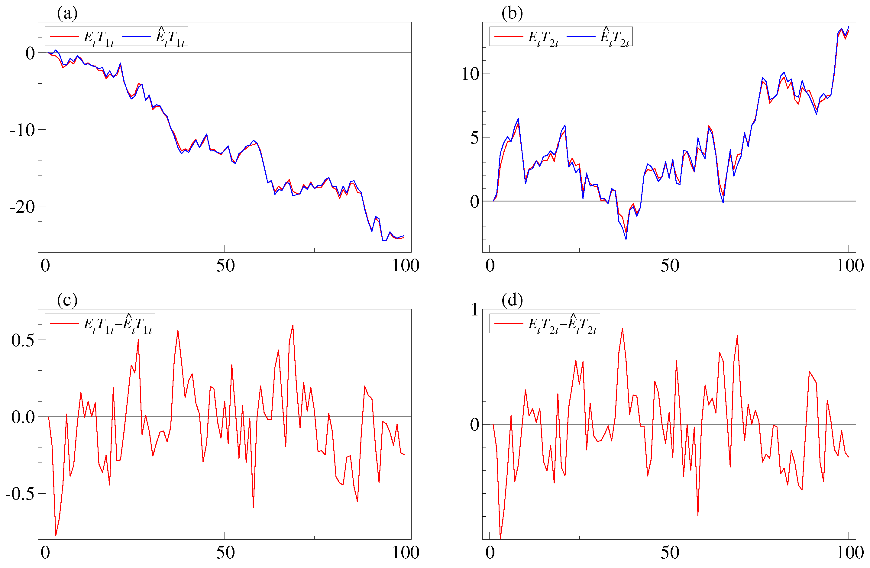
The parameters are estimated by (28) and the estimates become ${\widehat{b}}_{31}=0.48$, ${\widehat{b}}_{32}=0.41$, ${\widehat{\sigma }}_1^2=0.93$, ${\widehat{\sigma }}_{12}=0.26$, and ${\widehat{\sigma }}_2^2=1.63$. The extracted and estimated trends are plotted in Figure 1. Panels a and b show plots of $(E_t{T}_{1t},{\widehat{E}}_t{T}_{1t})$ and $(E_t{T}_{2t},{\widehat{E}}_t{T}_{2t})$, respectively, and it is seen that they co-move. In panels c and d the differences ${\widehat{E}}_t{T}_{1t}-E_t{T}_{1t}$ and ${\widehat{E}}_t{T}_{2t}-E_t{T}_{2t}$ both appear to be stationary in this parametrization of the model.      ■

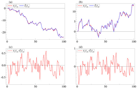
Figure 1. The figure shows the extracted and estimated trends for the simulated data in Example 1 with the identification in (19). Panels a and b show plots of $E_t{T}_{1t}$ and ${\widehat{E}}_t{T}_{1t}$, and $E_t{T}_{2t}$ and ${\widehat{E}}_t{T}_{2t}$, respectively. Note that in both cases, the processes seem to co-move. In panels c and d, $E_t{T}_{1t}-{\widehat{E}}_t{T}_{1t}$ and $E_t{T}_{2t}-{\widehat{E}}_t{T}_{2t}$ are plotted and appear stationary, because they are both recovered from $B{E}_t{T}_t-\widehat{B}{\widehat{E}}_t{T}_t$ as the first two coordinates, see (19).

Example 2 continued.

The parameter B in this example is given in (6) such that

$$E_{t}B{T}_t-{\widehat{E}}_t\widehat{B}{T}_t=\left(\begin{array}{c}{E}_t{T}_{1t}-{\widehat{E}}_t{T}_{1t}\\ b_{21}{E}_t{T}_{1t}+E_t{T}_{2t}-{\widehat{b}}_{21}{\widehat{E}}_t{T}_{1t}-{\widehat{E}}_t{T}_{2t}\\ b_{31}{E}_t{T}_{1t}+b_{32}{E}_t{T}_{2t}-{\widehat{b}}_{31}{\widehat{E}}_t{T}_{1t}-{\widehat{b}}_{32}{\widehat{E}}_t{T}_{2t}\end{array}\right).$$

(32)

By the results in Theorem 1(a), all three rows are asymptotically stationary, in particular $E_t{T}_{1t}-{\widehat{E}}_t{T}_{1t}$. Moreover, the second row of (32), $(b_{21}{E}_t{T}_{1t}-{\widehat{b}}_{21}{\widehat{E}}_t{T}_{1t})+(E_t{T}_{2t}-{\widehat{E}}_t{T}_{2t})$, is asymptotically stationary. Thus, asymptotic stationarity of $E_t{T}_{2t}-{\widehat{E}}_t{T}_{2t}$ requires asymptotic stationary of the term

$$b_{21}{E}_t{T}_{1t}-{\widehat{b}}_{21}{\widehat{E}}_t{T}_{1t}=(b_{21}-{\widehat{b}}_{21})E_t{T}_{1t}+{\widehat{b}}_{21}(E_t{T}_{1t}-{\widehat{E}}_t{T}_{1t}).$$

(33)

Here, the second term, ${\widehat{b}}_{21}(E_t{T}_{1t}-{\widehat{E}}_t{T}_{1t})$, is asymptotically stationary because $E_t{T}_{1t}-{\widehat{E}}_t{T}_{1t}$ is. However, the first term, $(b_{21}-{\widehat{b}}_{21})E_t{T}_{1t}$, is not asymptotically stationary because ${\widehat{b}}_{21}$ is $n^{1/2}$-consistent. In this case $n^{1/2}(b_{21}-{\widehat{b}}_{21})\stackrel{\mathrm{D}}{\to }Z$, which has a Gaussian distribution, and $n^{-1/2}{E}_{[nu]}{T}_{1[nu]}\stackrel{\mathrm{D}}{\to }{W}_{{\eta }_1}(u)$, where $W_{{\eta }_1}$ is the Brownian motion generated by the sum of ${\eta }_{1t}.$ It follows that their product

$$(b_{21}-{\widehat{b}}_{21})E_{[nu]}{T}_{1[nu]}=\{n^{1/2}(b_{21}-{\widehat{b}}_{21})\}\{n^{-1/2}{E}_{[nu]}{T}_{1[nu]}\}$$

converges in distribution to the product of Z and $W_{{\eta }_1}(u)$, $n\to \infty$, and this limit is nonstationary. It follows that $E_t{T}_{2t}-{\widehat{E}}_t{T}_{2t}$ is not asymptotically stationary for the identification in this example. This argument is a special case of the proof of Theorem 2.

To illustrate the results, data are simulated from the model with $n=100$ observations starting with $T_0=0$ and parameter values $b_{21}=0.0$, $b_{31}=b_{32}=0.5$, and ${\sigma }_1^2={\sigma }_2^2=1$, which is identical to (31).

The model is written in the form (19) with a transformed B and ${\mathrm{\Omega }}_{\eta },$ as

$$B^{†}=\left(\begin{array}{cc}1& 0\\ 0& 1\\ b_{31}-b_{32}{b}_{21}& b_{32}\end{array}\right),{\mathrm{\Omega }}_{\eta }^{†}=\left(\begin{array}{cc}{\sigma }_1^2& b_{21}{\sigma }_1^2\\ b_{21}{\sigma }_1^2& {\sigma }_2^2+b_{21}^2{\sigma }_1^2\end{array}\right).$$

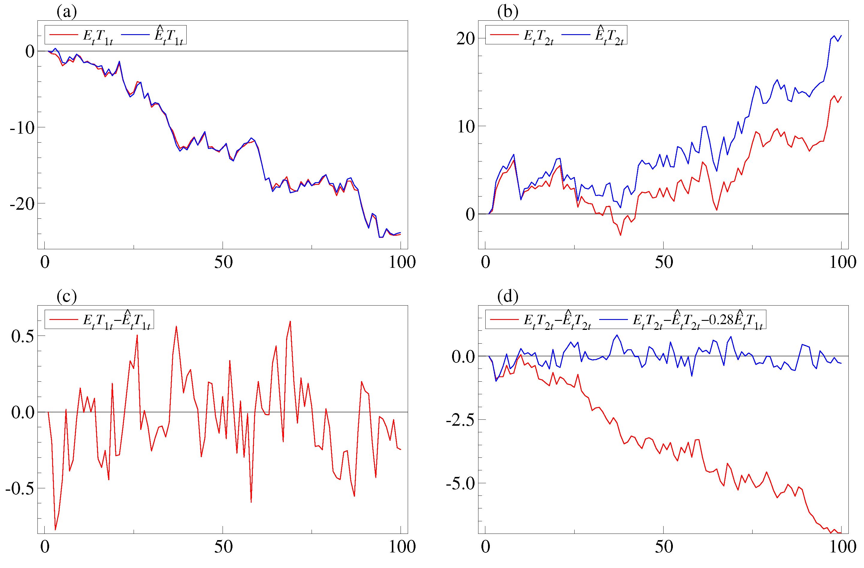
The parameters are estimed as in Example 1 and we find ${\widehat{b}}_{31}-{\widehat{b}}_{32}{\widehat{b}}_{21}=0.48$, ${\widehat{b}}_{32}=0.41$, ${\widehat{\sigma }}_1^2=0.93$, ${\widehat{b}}_{21}{\widehat{\sigma }}_{12}=0.26$, and ${\widehat{\sigma }}_2^2+{\widehat{b}}_{21}^2{\widehat{\sigma }}_1^2=1.63$, which are solved for ${\widehat{b}}_{21}=0.28$, ${\widehat{b}}_{31}=0.59$, ${\widehat{b}}_{32}=0.41$, ${\widehat{\sigma }}_1^2=0.93$, and ${\widehat{\sigma }}_2^2=1.56$. The extracted and estimated trends are plotted in Figure 2. The panels a and b show plots of $(E_t{T}_{1t},{\widehat{E}}_t{T}_{1t})$ and $(E_t{T}_{2t},{\widehat{E}}_t{T}_{2t})$, respectively. It is seen that $E_t{T}_{1t}$ and ${\widehat{E}}_t{T}_{1t}$ co-move, whereas $E_t{T}_{2t}$ and ${\widehat{E}}_t{T}_{2t}$ do not co-move. In panels c and d, the differences $E_t{T}_{1t}-{\widehat{E}}_t{T}_{1t}$ and $E_t{T}_{2t}-{\widehat{E}}_t{T}_{2t}$ are plotted. Note that the first looks stationary, whereas the second is clearly nonstationary. When comparing with the plot of $E_t{T}_{1t}$ in panel a, it appears that the process ${\widehat{E}}_t{T}_{1t}$ can explain the nonstationarity of $E_t{T}_{2t}-{\widehat{E}}_t{T}_{2t}$. This is consistent with Equation (33) with $b_{21}=0$ and ${\widehat{b}}_{21}=0.28$. In panel d, $E_t{T}_{2t}-{\widehat{E}}_t{T}_{2t}-0.28{\widehat{E}}_t{T}_{1t}$ is plotted and it is indeed stationary.      ■

Figure 2. The figure shows the extracted and estimated trends for the simulated data in Example 2 with the identification in (20). Panels a and b show plots of $E_t{T}_{1t}$ and ${\widehat{E}}_t{T}_{1t}$, and $E_t{T}_{2t}$ and ${\widehat{E}}_t{T}_{2t}$, respectively. Note that $E_t{T}_{1t}$ and ${\widehat{E}}_t{T}_{1t}$ seem to co-move, whereas $E_t{T}_{2t}$ and ${\widehat{E}}_t{T}_{2t}$ do not. In panel $c,$$E_t{T}_{1t}-{\widehat{E}}_t{T}_{1t}$ is plotted and appears stationary, but in panel d the spread $E_t{T}_{2t}-{\widehat{E}}_t{T}_{2t}$ is nonstationary, whereas $E_t{T}_{2t}-{\widehat{E}}_t{T}_{2t}-0.28{\widehat{E}}_t{T}_{1t}$ is stationary.

6. Conclusions

The paper analyses a sample of n observations from a common trend model, where the state is an unobserved multivariate random walk and the observation is a linear combination of the lagged state variable and a noise term. For such a model, the trends and their coefficients in the observation equation need to be identified before they can be estimated separately. The model leads naturally to cointegration between observations, trends, and the extracted trends. Using simulations it was discovered, that the extracted trends do not necessarily cointegrate with their estimators. This problem is investigated, and it is found to be related to the identification of the trends and their coefficients in the observation equation. It is shown in Theorem 1, that provided only the linear combinations of the trends from the observation equation are considered, there is always cointegration between extracted trends and their estimators. If the trends and their coefficients are defined by identifying restrictions, the same result holds if and only if the estimated identified coefficients in the observation equation are consistent at a rate faster than $n^{1/2}$. For the causality study mentioned in the introduction, where the components of the unobserved trend are assumed independent, the result has the following implication: For the individual extracted trends to cointegrate with their estimators, overidentifying restrictions must be imposed on the trend’s causal impact coefficients on the observations, such that the estimators of these become super-consistent.

References

- Chan, Siew Wah, Graham Clifford Goodwin, and Kwai Sang Sin. 1984. Convergence properties of the Ricatti difference equation in optimal filtering of nonstabilizable systems. IEEE Transaction on Automatic Control 29: 110–18. [Google Scholar] [CrossRef]
- Durbin, Jim, and Siem Jan Koopman. 2012. Time Series Analysis by State Space Methods, 2nd ed. Oxford: Oxford University Pres. [Google Scholar]
- Fisher Frank, M. 1966. The Identification Problem in Econometrics. New York: McGraw-Hill. [Google Scholar]
- Harvey, Andrew. 1989. Forecasting, Structural Time Series Models and the Kalman Filter. Cambridge: Cambridge University Press. [Google Scholar]
- Harvey, Andrew C. 2006. Forecasting with Unobserved Components Time Series Models. In Handbook of Economic Forecasting. Edited by G. Elliot, C. Granger and A. Timmermann. Amsterdam: North Holland, pp. 327–412. [Google Scholar]
- Harvey, Andrew C., and Siem Jan Koopman. 1997. Multivariate structural time series models. In System Dynamics in Economics and Financial Models. Edited by C. Heij, J.M. Schumacher, B. Hanzon and C. Praagman. New York: John Wiley and Sons. [Google Scholar]
- Hoover, Kevin D., Søren Johansen, Katarina Juselius, and Morten Nyboe Tabor. 2014. Long-run Causal Order: A Progress Report. Unpublished manuscript. [Google Scholar]
- Johansen, Søren. 1996. Likelihood-Based Inference in Cointegrated Vector Autoregressive Models, 2nd ed. Oxford: Oxford University Press. [Google Scholar]
- Johansen, Søren. 2010. Some identification problems in the cointegrated vector autoregressive model. Journal of Economietrics 158: 262–73. [Google Scholar] [CrossRef]
- Johansen, Søren, and Katarina Juselius. 2014. An asymptotic invariance property of the common trends under linear transformations of the data. Journal of Econometrics 178: 310–15. [Google Scholar] [CrossRef]
- Pearl, Judea. 2009. Causality: Models, Reasoning and Inference, 2nd ed. Cambridge: Cambridge University Press. [Google Scholar]
- Saikkonen, Pentti. 1992. Estimation and testing of cointegrated systems by an autoregressive approximation. Econometric Theory 8: 1–27. [Google Scholar] [CrossRef]
- Saikkonen, Pentti, and Helmut Lütkepohl. 1996. Infinite order cointegrated vector autoregressive processes. Estimation and Inference. Econometric Theory 12: 814–44. [Google Scholar] [CrossRef]
- Spirtes, Peter, Clark Glymour, and Richard Scheines. 2000. Causation, Prediction, and Search, 2nd ed. Cambridge: MIT Press. [Google Scholar]
© 2017 by the authors. Licensee MDPI, Basel, Switzerland. This article is an open access article distributed under the terms and conditions of the Creative Commons Attribution (CC BY) license (http://creativecommons.org/licenses/by/4.0/).