On The Interpretation of Instrumental Variables in the Presence of Specification Errors: A Causal Comment

Abstract

Swamy et al. (2015) argue that valid instruments cannot exist when a structural model is misspecified. This note shows that this is not true in general. In simple examples valid instruments can exist and can help to estimate parameters of interest.

1. Introduction

Does an efficient financial system enhance growth? Does uncertainty depress private investment? Do private schools provide better education than public schools? In answering these and many other empirical questions instrumental variables play a central role.

In a recent paper Swamy et al. (2015) argue that valid instruments cannot exist in the presence of any model misspecification. Such mis-specifications include wrong functional form, omission of relevant explanatory variables, and the presence of measurement error in explanatory variables. As a consequence, instrumental variables (IV) and generalized method of moments (GMM) would not work.

No doubt, instruments may be hard to find or difficult to justify in empirical applications. The claim that instruments cannot exist appears to be too strong, however. This note discusses three simple examples where valid instruments can exist and where IV methods will work.

This note proceeds as follows. The next section reproduces the derivations in Swamy et al. (2015) for a simple linear model. This example helps to explain the logic of their nonexistence result for instrumental variables.

Section 3 briefly discusses the nature of structural models. The aim is to clarify some misconceptions that bedevil the interpretation of structural models.

Section 4 reexamines the basic arguments of Swamy et al. (2015) in the context of three extremely simple structural models. All three regressions for estimating the structural parameter of interest are misspecified in these cases. In the first two cases one of the two explanatory variables has been omitted. In the third case the single explanatory variable contains measurement error.

The following will be shown. In the first case the existence of a valid instruments depends on the purpose of the analysis. In the second case instruments can exist and will produce consistent estimates of the structural parameter of interest. In the third example instruments can solve the measurement error problem.

2. Non-Existence of Instruments

The central argument in Swamy et al. (2015) is that the explanatory variables that must be instrumented in an empirical model to obtain consistent estimates are at the same time also part of the error term of the model. All potential instruments are therefor necessarily correlated with the error term. The requirement that instruments must be uncorrelated with the error term is always violated. Hence, valid instruments cannot exist.

Swamy et al. (2015) start with a very general theoretical relationship

$$y_t^{*}=f_t(x_{1t}^{*},...,x_{L(t)t}^{*})$$

(1)

with unknown functional form, where a possibly time dependent number $L(t)$ of variables $x_{it}^{*}$ determine $y_t^{*}$. This theoretical relationship is assumed to be exact. Thus there is no need for an error term.

The derivations in Swamy et al. (2015) are now repeated for a simple linear model where $y_t^{*}$ is exactly determined by two variables $x_{1t}^{*}$ and $x_{2t}^{*}$. This model can be written as

$$y_t^{*}={\alpha }_0+{\alpha }_1{x}_{1t}^{*}+{\alpha }_2{x}_{2t}^{*}.$$

(2)

Equation (2) is the true model.

Let us assume that we can only observe the measurements $y_t=y_t^{*}+{\nu }_{0t}$ and $x_{1t}=x_{1t}^{*}+{\nu }_{1t}$ where ${\nu }_{0t}$ and ${\nu }_{1t}$ are measurement errors. Thus, the model that we can estimate has the correct functional form, but suffers from measurement error and an omitted variable.

Swamy et al. (2015) argue that the relationship between the unobserved and the observed determinant can always be written as

$$x_{2t}^{*}={\lambda }_{0t}+{\lambda }_{1t}{x}_{1t}^{*}$$

(3)

where ${\lambda }_{0t}$ is the portion of $x_{2t}^{*}$ that remains after the effect of $x_{1t}^{*}$ is removed. Substituting (3) into (2) yields

$$y_t^{*}={\alpha }_0+{\alpha }_2{\lambda }_{0t}+({\alpha }_1+{\alpha }_2{\lambda }_{1t})x_{1t}^{*}.$$

(4)

Accounting for the measurement errors in (4) gives

$$y_t={\alpha }_0+{\alpha }_2{\lambda }_{0t}+{\nu }_{0t}+({\alpha }_1+{\alpha }_2{\lambda }_{1t})(1-\frac{{\nu }_{1t}}{x_{1t}})x_{1t}$$

(5)

This equation includes the bias arising from omitting $x_{2t}^{*}$, the bias from measurement error in $x_{1t}$, and the measurement error in $y_t$. It is a simple version of the fully general expression (8) in Swamy et al. (2015). This model can be written as $y_t={\gamma }_{0t}+{\gamma }_{1t}{x}_{1t}$ where the parameters ${\gamma }_{0t}={\alpha }_0+{\alpha }_2{\lambda }_{0t}+{\nu }_{0t}$ and ${\gamma }_{1t}=({\alpha }_1+{\alpha }_2{\lambda }_{1t})(1-\frac{{\nu }_{1t}}{x_{1t}})$ are time-varying.

Let us now consider two of the cases discussed in Swamy et al. (2015). In the first case the model is linear. Adding and subtracting the constant parameter model ${\beta }_0+{\beta }_1{x}_{1t}$ to (5) yields

$$y_t={\beta }_0+{\beta }_1{x}_{1t}+({\alpha }_0+{\alpha }_2{\lambda }_{0t}+{\nu }_{0t}-{\beta }_0+({\alpha }_1+{\alpha }_2{\lambda }_{1t})(1-\frac{{\nu }_{1t}}{x_{1t}})-{\beta }_1)x_{1t})$$

(6)

where the last two terms become the error term in the model to be estimated. A valid instrument must be correlated with $x_{1t}$ and uncorrelated with the error term. But $x_{1t}$ is also in the error term of (6). Thus, every instrument for $x_{1t}$ must be correlated with the error. No valid instrument exists in model (6).

The other case is a simple example of a model with a measurement error in the explanatory variable. This model is

$$y_t^{*}=\beta x_t^{*}$$

(7)

where the measured value of the explanatory variable is $x_t=x_t^{*}+{\nu }_t$. The model that can be estimated is

$$y_t^{*}=\beta x_t-\beta {\nu }_t$$

(8)

where $-\beta {\nu }_t$ is the error term. Written as time-varying coefficient model (8) becomes

$$y_t^{*}={\beta }_t{x}_t$$

(9)

where ${\beta }_t=\beta (1-\frac{{\nu }_t}{x_t})$. Adding and subtracting a fixed coefficient model where ${\beta }^{**}\ne \beta$ yields

$$y_t^{*}={\beta }^{**}{x}_t+({\beta }_t-{\beta }^{**})x_t$$

(10)

and $x_t$ is again also in the error term of Equation (8). No instrument for $x_t$ would work.

3. Structural Models

Before we reexamine the arguments in Section 2 we need to clarify what structural models are and what kind of assumptions they encode. This note cannot give a full exposition, of course. Pearl (2009a) provides a comprehensive treatment of structural models and causal inference in general. In particular, Chapter 5 in Pearl (2009a) discusses the interpretation of structural parameters and the error term in structural models in great detail. This section draws heavily on Pearl (2009b) which gives an excellent overview of the foundations of causal modeling with structural equations.

Let us consider the simple linear structural equation

$$y=\beta x+{\nu }_0.$$

(11)

where y depends on x and ${\nu }_0$, a variable that stands for all other factors that affect y when x is held constant. Particular values of x and ${\nu }_0$ assign a particular value $y=\beta x+{\nu }_0$.

Equation (11) encodes the causal assumption that changing or manipulating x causes y to vary. The strength of the this effect is $\beta$. Note that the interpretation of $\beta$ does not depend on ${\nu }_0$. The equation says that the effect of a unit change in x on y is $\beta$, regardless of the values taken by the other variables in the model. Whether or not x is correlated with ${\nu }_0$ plays no role. Equation (11) describes a causal mechanism, not statistical associations. The correlation between x and ${\nu }_0$ becomes important, however, when one attempts to estimate the causal parameter $\beta$ from observational data.

Furthermore, the relation between x and y is asymmetric. The equality sign is therefore somewhat misleading. Rewriting (11) as

$$x=(y-{\nu }_0)/\beta$$

(12)

would lead to the miss-interpretation that y causes x. For example, when y is a symptom of a disease x than (12) would imply that the symptom causes the disease. This makes of course no sense.

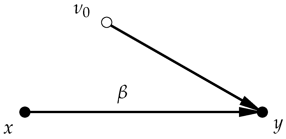
The graph in Figure 1 makes the causal relationship between x and y explicit. The arrow that points from x to y shows the direction of causality between these variables. The solid nodes indicate that x and y are observable variables. The hollow node indicates that the variable ${\nu }_0$ is unobserved. The absence of a link between x and ${\nu }_0$ in this graph indicate the these two variables are assumed to be independent.

Another important assumption in Equation (11) is the invariance of the target parameter $\beta$. This is an identifying assumption. The assumption implies that the causal link between x and y is stable. One could of course assume that $\beta$ changes over time in some way. But this would imply a very different structural model.

Until now nothing was said about estimating Equation (11). The question is whether the causal effect $\beta$ can be estimated from observational data. When x is uncorrelated with ${\nu }_0$ then $\beta$ is identified and consistently estimable from data on y and x. When x and ${\nu }_0$ are dependent, however, then we need additional information to consistently estimate $\beta$. This information may come from an instrumental variable.

4. Non-Existence Revisited: Instruments Do Exist

Let us now turn again to our simple model given by Equation (2) and let us assume that we can only observe $y^{*}$ and $x_1^{*}$. We cannot observe $x_2^{*}$. For simplicity the intercept ${\alpha }_0$ is set to zero. The time subscript t is superfluous and therefore dropped.

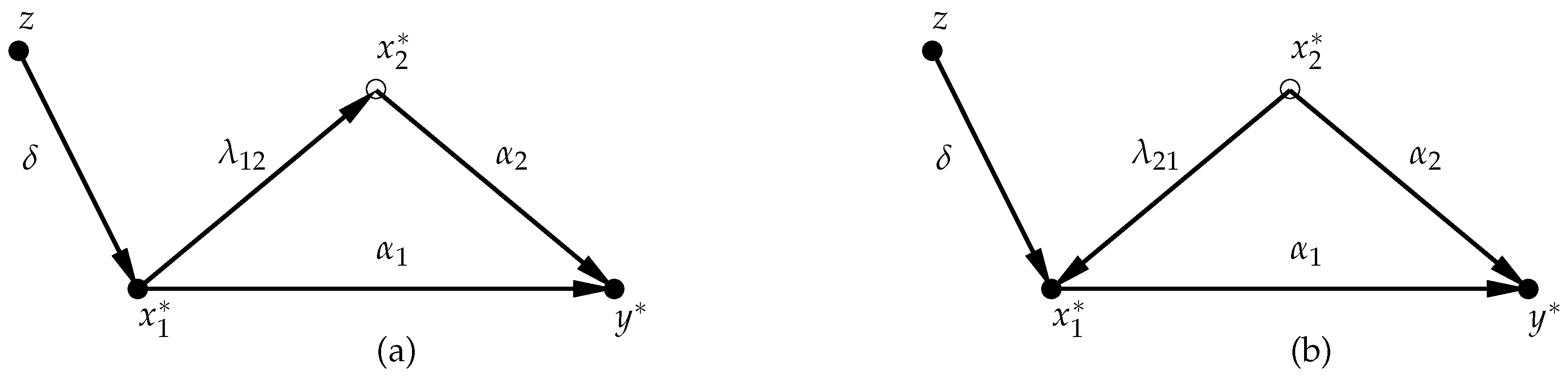
Figure 2 shows two possible structural models. In model (a) $x_1^{*}$ affects $y^{*}$ directly and indirectly via its effect on $x_2^{*}$. In model (b) the variable $x_2^{*}$ is a confounding variable that jointly affects $y^{*}$ and $x_1^{*}$. In both graphs z is an instrumental variable.

The regression model that is actually estimated is

$$y^{*}=\beta x_1^{*}+ϵ$$

(13)

where the error term $ϵ={\alpha }_2{x}_2^{*}$. Thus, the model is misspecified because $x_2^{*}$ is omitted. In both cases $x_1^{*}$ is correlated with the error. Let us now compute the ordinary least squares (OLS) and IV estimates for both cases.

Case (a): Easy computations show that OLS yields

$${\beta }_{(a)}^{OLS}=\frac{Cov(y^{*},x_1^{*})}{Var(x_1^{*})}=\frac{({\alpha }_1+{\alpha }_2{\lambda }_{12})Var(x_1^{*})}{Var(x_1^{*})}={\alpha }_1+{\alpha }_2{\lambda }_{12}$$

(14)

This is the total (i.e., direct + indirect) effect of $x_1^{*}$ on $y^{*}$. The IV estimate for $\beta$ is

$${\beta }_{(a)}^{IV}=\frac{Cov(y^{*},z)}{Cov(x_1^{*},z)}=\frac{({\alpha }_1+{\alpha }_2{\lambda }_{12})\delta Var(z)}{\delta Var(z)}={\alpha }_1+{\alpha }_2{\lambda }_{12}$$

(15)

and therefore the same as the OLS estimate. When the goal is to estimate only the direct effect of $x_1^{*}$ on $y^{*}$ no instrument for $x_1^{*}$ works as argued in Swamy et al. (2015). If one is interested in the total effect no instrument is needed anyway.

Case (b): Now $x_2^{*}$ is a confounding variable. As already mentioned, this model is miss-specified and Swamy et al. (2015) would conclude that a valid instrument cannot exist. But in fact a valid instrument can exist. OLS wont work but IV estimation will.

OLS yields

$${\beta }_{(b)}^{OLS}=\frac{{\alpha }_1{\lambda }_{21}^{2}Var(x_2^{*})+{\alpha }_2{\lambda }_{21}Var(x_2^{*})}{{\lambda }_{21}^{2}Var(x_2^{*})}={\alpha }_1+{\alpha }_2(1/{\lambda }_{21})$$

(16)

where the second term is the well known omitted variable bias. The term $(1/{\lambda }_{21})$ is the coefficient from a regression of $x_2^{*}$ on $x_1^{*}$. Note that this auxiliary regression has no causal content. The regression just measures the statistical association between $x_2^{*}$ and $x_1^{*}$. Some simple algebra shows that IV estimation yields now

$${\beta }_{(b)}^{IV}=\frac{{\alpha }_1\delta Var(z)}{\delta Var(z)}={\alpha }_1$$

(17)

which is the structural parameter that we wanted to estimate.

Why can an instrument work in case (b) but not in case (a)? In case (a) the error term $ϵ={\alpha }_2{x}_2^{*}={\alpha }_2{\lambda }_{12}{x}_1^{*}$ is caused by the included variable. The error term is thus indeed a function of $x_1^{*}$. No instrument for $x_1^{*}$ will therefore work if one wants to estimate the direct effect of $x_1^{*}$ on $y^{*}$.

Case (b) is quite different. in Figure 2b the error is not a function of the included explanatory variable. Equation (3) in Section 2 is thus not consistent with the underlying structural model. Varying $x_1^{*}$ does not affect $x_2^{*}$. Instead the omitted variable $x_2^{*}$ in the error term is a cause of the explanatory variable $x_1^{*}$. The instrument z is another cause of $x_1^{*}$ that is independent of $x_2^{*}$. Thus the error and the instrument are uncorrelated. Moreover, the instrument affects the dependent variable $y^{*}$ only via $x_1^{*}$. IV estimation works with a proper instrument.

Let us now turn to the second example in Section 2 where $y_t^{*}=\beta x_t^{*}$ and the explanatory variable $x_t=x_t^{*}+{\nu }_t$ is measured with error. If $y_t^{*}=\beta x_t^{*}$ is the true structural model then the causal effect of $x_t^{*}$ on $y_t^{*}$ is stable. The constant parameter $\beta$ reflects this. Hence, we cannot simply transform this model into a time-varying coefficient model. Such a model states that the causal effect is unstable and changes over time. The transformed model is therefore inconsistent with the true structural model that we want to estimate. The transformed model has very different implications for the causal link between $x_t^{*}$ and $y_t^{*}$. It is a different structural model.

To be consistent with the original structural model one should estimate the model $y_t^{*}=\beta x_t-\beta {\nu }_t$. Here the error is not a function of $x_t$ and instruments can in principle be found. For example, any cause of $x_t^{*}$ that is unrelated to the measurement error ${\nu }_t$ and does not directly cause $y_t^{*}$ would be a valid instrument for $x_t$.

5. Conclusions

The examples presented in this note demonstrate that instruments can exist. The arguments in Swamy et al. (2015) hold when the structural error is indeed a function of the included explanatory variables. But this is rarely the case in a structural model. For instance, omitted confounding variables are not functions of included variables. The three variable model (b) in Figure 2 provides a simple example. The model is misspecified, but a valid instrument exists since the omitted confounding variable is not a function of the included variable.

Furthermore, Swamy et al. (2015) assume that any model can be expressed as a time varying coefficient (TVC) model. The true model would then be a special case of this general model.

Of course, a constant parameter model is a special case of a TVC model. A true structural model with constant parameters cannot be turned into an equivalent TVC model, however. A structural model with constant parameters cannot at the same time be expressed as a model where the parameters vary over time. The later model has very different causal implications.