
The Evolving Transmission of Uncertainty Shocks in the United Kingdom

Abstract
:1. Introduction
2. Empirical Model
3. Estimation and Model Specification
3.1. Priors and Starting Values
3.1.1. VAR Coefficients
3.1.2. Elements of the A Matrix
3.1.3. Elements of S and the Parameters of the Stochastic Volatility Transition Equation
3.1.4. Common Volatility
3.2. MCMC Algorithm
- The distribution of the time-varying VAR coefficients conditional on all other parameters Ξ is linear and Gaussian: and , where Ξ denotes a vector that holds all of the other VAR parameters. As shown by [16] the simulation proceeds as follows. First, we use the Kalman filter to draw and and then proceed backwards in time using and
- . The conditional posterior for is inverse Wishart: , i.e., the posterior scale matrix is given by , and the degrees of freedom are .
- Given a draw for the VAR parameters, the model can be written as , where denotes the VAR residuals. This is a system of linear equations with time-varying coefficients and a known form of heteroscedasticity. The j-th equation of this system is given as , where the subscript j denotes the j-th column of v, while denotes Columns 1 to . Note that the variance of is time-varying and given by . The time-varying coefficient follows the process with the shocks to the j-th equation uncorrelated with those from other equations. In other words, the covariance matrix is assumed to be block diagonal, as in [5]. With this assumption in place, the [16] algorithm can be applied to draw the time varying coefficients for each equation of this system separately.
- . Given a draw for the VAR parameters, the model can be written as The j-th equation of this system is given by , where the variance of is time-varying and given by Given a draw for , this equation can be re-written as , where , and the variance of is . The conditional posterior for this variance is inverse Gamma with scale parameter and degrees of freedom
- Conditional on the VAR parameters, and the parameters of the transition equation, the model has a multivariate non-linear state-space representation. The work in [17] shows that the conditional distribution of the state variables in a general state-space model can be written as the product of three terms:where Ξ denotes all other parameters and . In the context of stochastic volatility models, [18] show that this density is a product of log normal densities for and and a normal density for The work in [17] derives the general form of the mean and variance of the underlying normal density for and shows that this is given as:where and Note that due to the non-linearity of the observation equation of the model, an analytical expression for the complete conditional is unavailable, and a Metropolis step is required. Following [18], we draw from Equation (6) using a date-by-date independence Metropolis step using the density in Equation (7) as the candidate generating density. This choice implies that the acceptance probability is given by the ratio of the conditional likelihood at the old and the new draw. To implement the algorithm, we begin with an initial estimate of . We set the matrix equal to the initial volatility estimate. Then, at each date, the following two steps are implemented:
- (a)
- Draw a candidate for the volatility using the density 6, where and .
- (b)
- Update with acceptance probability , where is the likelihood of the VAR for observation t and defined as , where and .
Repeating these steps for the entire time series delivers a draw of the stochastic volatilities.3 - We re-write the transition equation in deviations from the mean:where the elements of the mean vector are defined as Conditional on a draw for and μ, the transition Equation (8) is simply a linear regression, and the standard normal and inverse Gamma conditional posteriors apply. Consider and The conditional posterior of F is , where:The conditional posterior of is inverse Gamma with scale parameter and degrees of freedom .Given a draw for F, Equation (8) can be expressed as , where and The conditional posterior of μ is , where:Note that α can be recovered as .
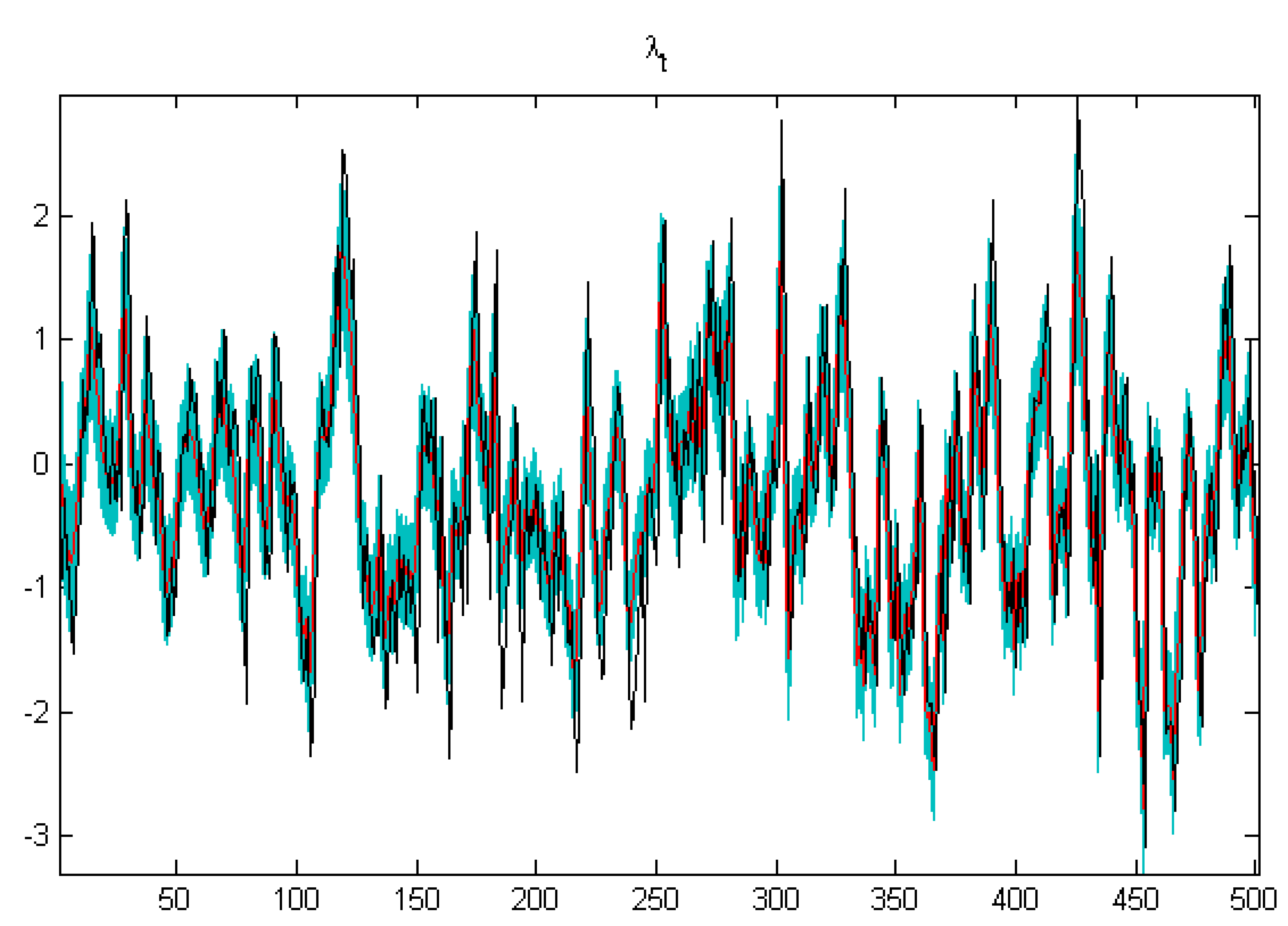
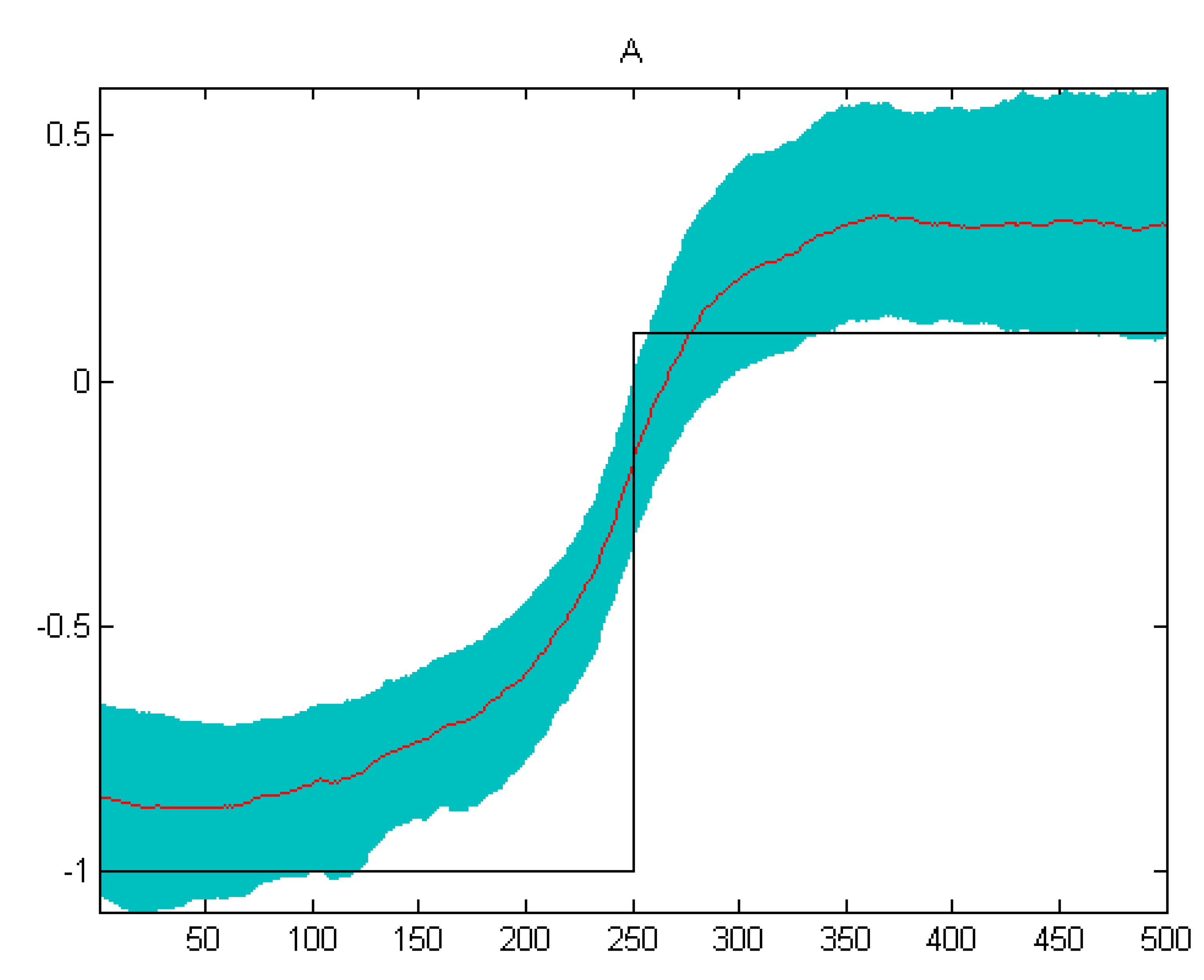
3.3. Estimation Using Artificial Data
4. Empirical Analysis for the U.K.
4.1. Data
4.2. Model Specification
4.3. Empirical Results
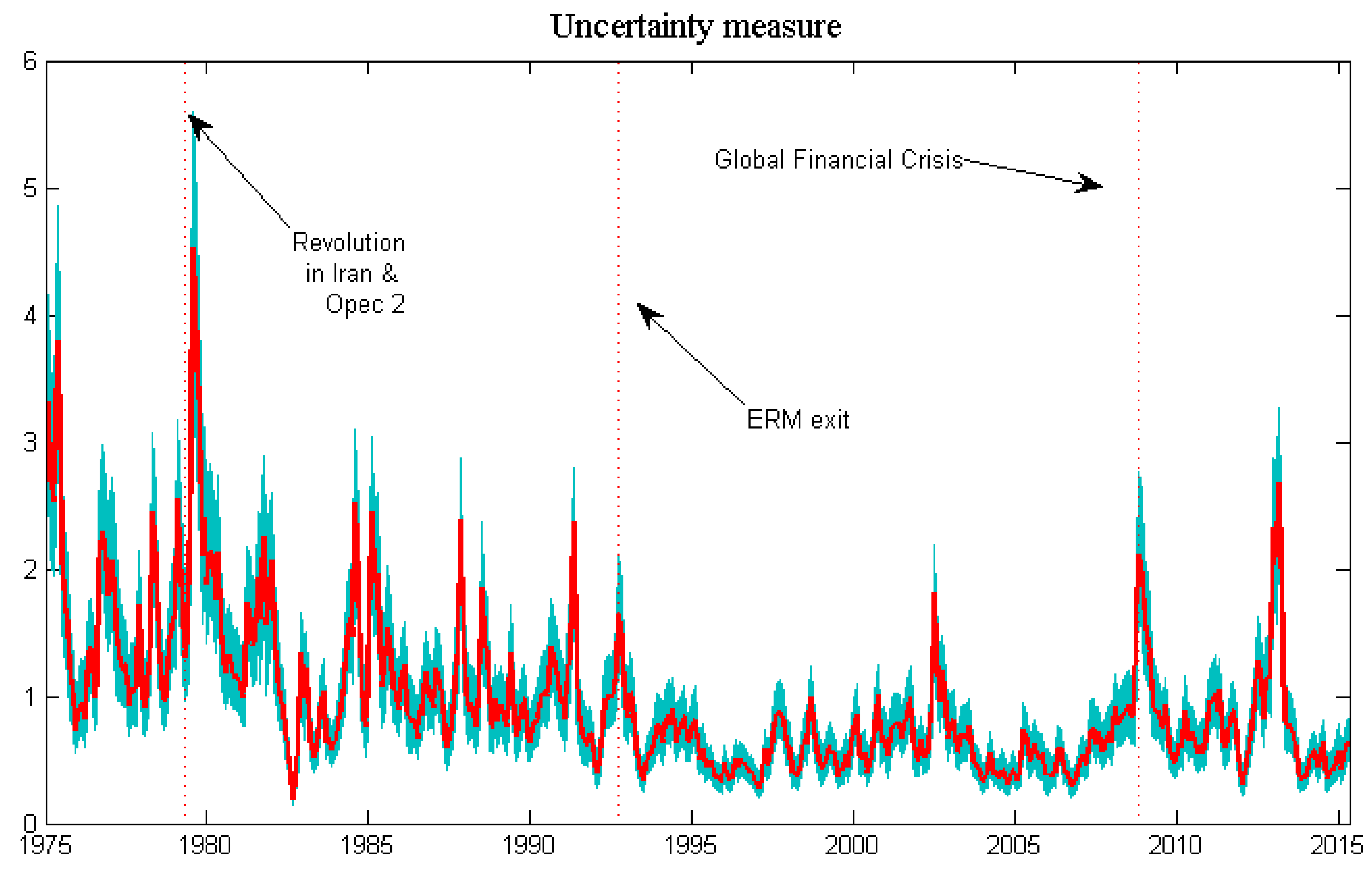
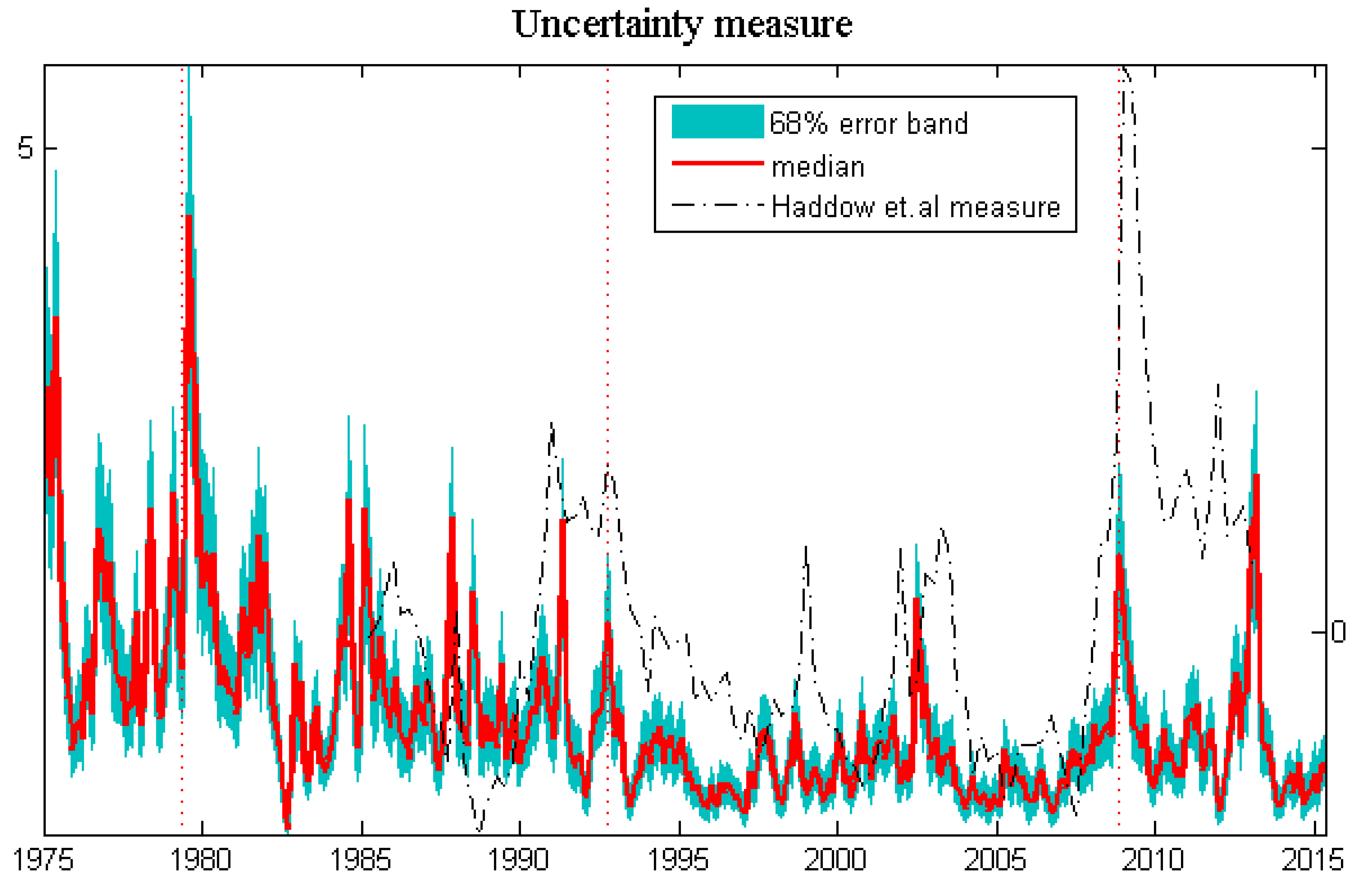
4.3.1. Estimated Volatility
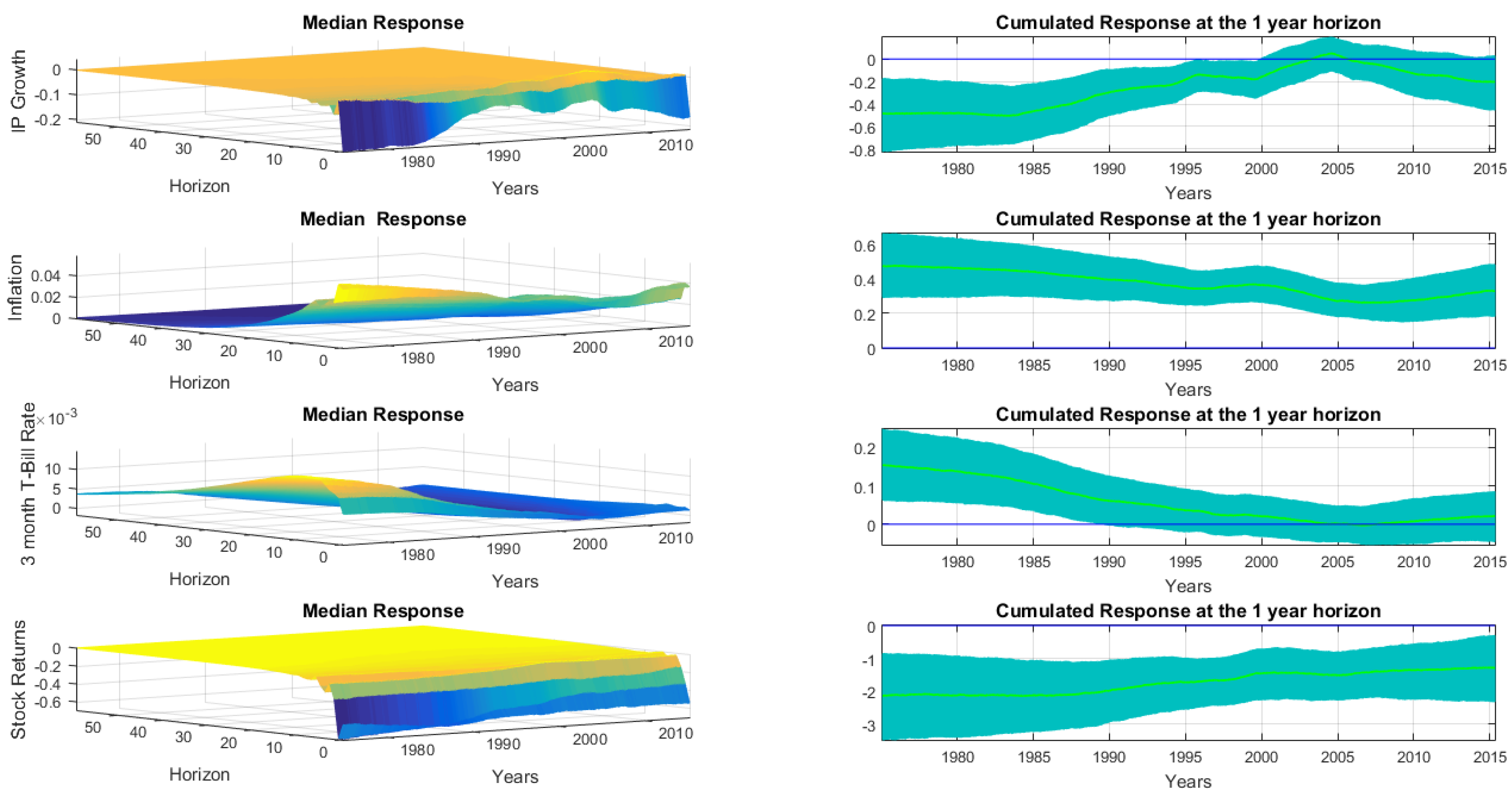
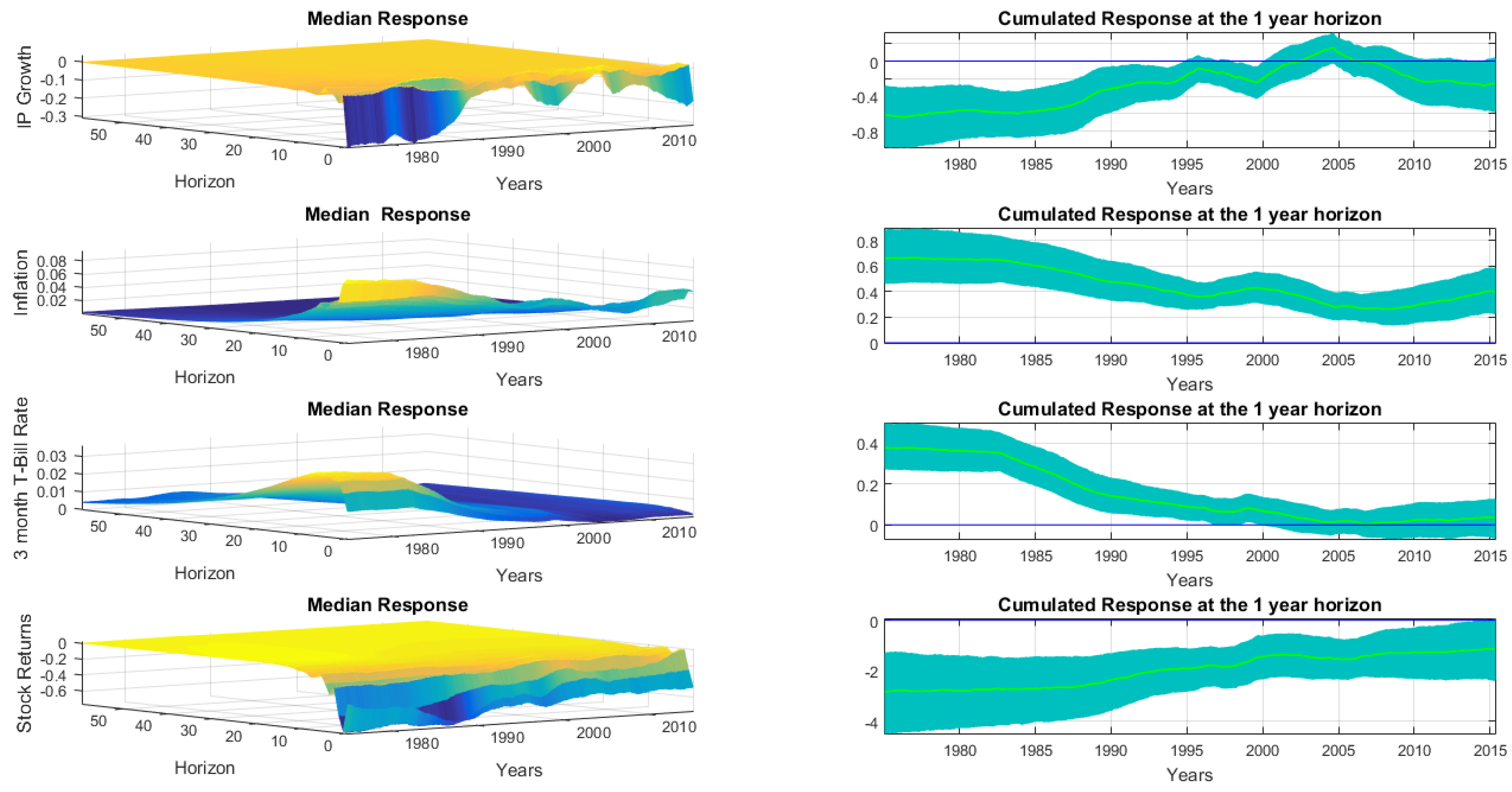
4.3.2. Impulse Response to Volatility Shocks
5. Conclusions
Acknowledgments
Conflicts of Interest
Appendix
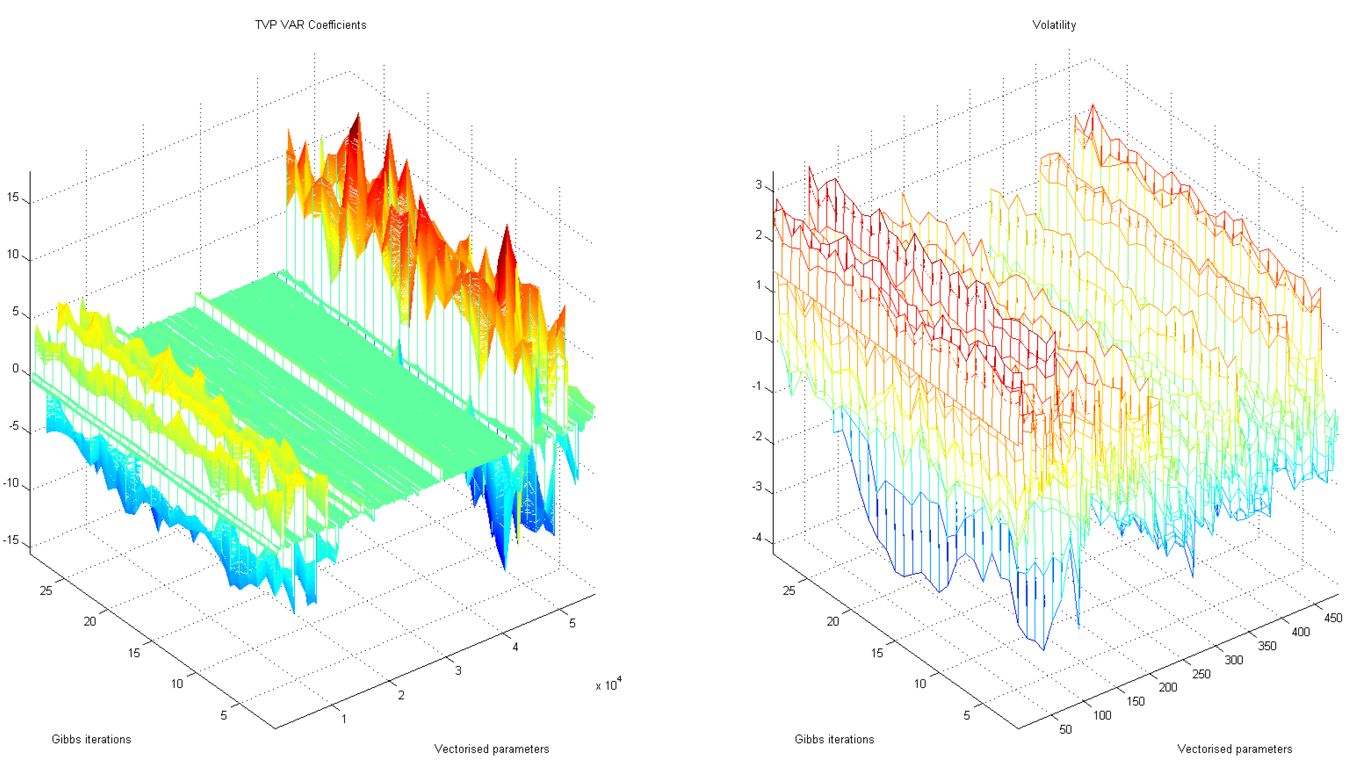
A. Convergence
B. Sensitivity Analysis

References
- N. Bloom. “The Impact of Uncertainty Shocks.” Econometrica 77 (2009): 623–685. [Google Scholar]
- S. Denis, and P. Kannan. The Impact of Uncertainty Shocks on the UK Economy. IMF Working Papers 13/66; Washington, DC, USA: International Monetary Fund, 2013. [Google Scholar]
- R. Beetsma, and M. Giuliodori. “The changing macroeconomic response to stock market volatility shocks.” J. Macroecon. 34 (2012): 281–293. [Google Scholar] [CrossRef]
- H. Mumtaz, and K. Theodoridis. The Changing Transmission of Uncertainty shocks in the US: An Empirical Analysis. Working Papers 735; London, UK: Queen Mary University of London, School of Economics and Finance, 2014. [Google Scholar]
- G. Primiceri. “Time varying structural vector autoregressions and monetary policy.” Rev. Econ. Stud. 72 (2005): 821–852. [Google Scholar] [CrossRef]
- A. Carriero, T.E. Clark, and M. Marcellino. “Common Drifting Volatility in Large Bayesian VARs.” J. Bus. Econ. Stat., 2015. [Google Scholar] [CrossRef]
- T. Cogley, and T.J. Sargent. “Drifts and Volatilities: Monetary policies and outcomes in the Post WWII U.S.” Rev. Econ. Dyn. 8 (2005): 262–302. [Google Scholar] [CrossRef]
- S.J. Koopman, and E. Hol Uspensky. “The stochastic volatility in mean model: Empirical evidence from international stock markets.” J. Appl. Econom. 17 (2002): 667–689. [Google Scholar] [CrossRef]
- H. Berument, Y. Yalcin, and J. Yildirim. “The effect of inflation uncertainty on inflation: Stochastic volatility in mean model within a dynamic framework.” Econ. Model. 26 (2009): 1201–1207. [Google Scholar] [CrossRef]
- L. Kwiatkowski. “Markov Switching In-Mean Effect. Bayesian Analysis in Stochastic Volatility Framework.” Cent. Eur. J. Econ. Model. Econ. 2 (2010): 59–94. [Google Scholar]
- M. Lemoine, and C. Mougin. The Growth-Volatility Relationship: New Evidence Based on Stochastic Volatility in Mean Models. Working Paper 285; Paris, France: Banque de France, 2010. [Google Scholar]
- M. Asai, and M. McAleer. “Multivariate stochastic volatility, leverage and news impact surfaces.” Econom. J. 12 (2009): 292–309. [Google Scholar] [CrossRef]
- B. Aruoba, L. Bocola, F. Schorfheide, and Department of Economics, University of Maryland. “A New Class of Nonlinear Times Series Models for the Evaluation of DSGE Models.” 2011, unpublished work. [Google Scholar]
- H. Mumtaz, and K. Theodoridis. “The international transmission of volatility shocks: An empirical analysis.” J. Eur. Econ. Assoc. 13 (2015): 512–533. [Google Scholar] [CrossRef]
- L. Benati, and H. Mumtaz. U.S. evolving macroeconomic dynamics—A structural investigation. Working Paper Series 746; Frankfurt am Main, Germany: European Central Bank, 2007. [Google Scholar]
- C. Carter, and P. Kohn. “On Gibbs sampling for state space models.” Biometrika 81 (2004): 541–553. [Google Scholar] [CrossRef]
- B.P. Carlin, N.G. Polson, and D.S. Stoffer. “A Monte Carlo Approach to Nonnormal and Nonlinear State-Space Modeling.” J. Am. Stat. Assoc. 87 (1992): 493–500. [Google Scholar] [CrossRef]
- E. Jacquier, N. Polson, and P. Rossi. “Bayesian analysis of stochastic volatility models.” J. Bus. Econ. Stat. 12 (1994): 371–418. [Google Scholar]
- J.A. Gamble, and J.P. LeSage. “A Monte Carlo Comparison of Time Varying Parameter and Multiprocess Mixture Models in the Presence of Structural Shifts and Outliers.” Rev. Econ. Stat. 75 (1993): 515–519. [Google Scholar] [CrossRef]
- A. Haddow, C. Hare, J. Hooley, and T. Shakir. “Macroeconomic uncertainty: What is it, how can we measure it and why does it matter? ” Bank Engl. Q. Bull. 53 (2013): 100–109. [Google Scholar]
- T. Cogley, and T.J. Sargent. “Anticipated utility and rational expectations as approximations of bayesian decision making.” Int. Econ. Rev. 49 (2008): 185–221. [Google Scholar] [CrossRef]
- J. Fernández-Villaverde, K.K. Pablo Guerrón-Quintana, and J. Rubio-Ramírez. “Fiscal Volatility Shocks and Economic Activity.” Am. Econ. Rev. 105 (2015): 3352–3384. [Google Scholar] [CrossRef]
- E. Nelson. UK Monetary Policy 1972-97: A Guide Using Taylor Rules. CEPR Discussion Paper 2931; London, UK: Centre for Economic Policy Research, 2001. [Google Scholar]
- 3.In order to take endpoints into account, the algorithm is modified slightly for the initial condition and the last observation. Details of these changes can be found in [18].


© 2016 by the author; licensee MDPI, Basel, Switzerland. This article is an open access article distributed under the terms and conditions of the Creative Commons by Attribution (CC-BY) license ( http://creativecommons.org/licenses/by/4.0/).
Share and Cite
Mumtaz, H. The Evolving Transmission of Uncertainty Shocks in the United Kingdom. Econometrics 2016, 4, 16. https://doi.org/10.3390/econometrics4010016
Mumtaz H. The Evolving Transmission of Uncertainty Shocks in the United Kingdom. Econometrics. 2016; 4(1):16. https://doi.org/10.3390/econometrics4010016
Chicago/Turabian StyleMumtaz, Haroon. 2016. "The Evolving Transmission of Uncertainty Shocks in the United Kingdom" Econometrics 4, no. 1: 16. https://doi.org/10.3390/econometrics4010016
APA StyleMumtaz, H. (2016). The Evolving Transmission of Uncertainty Shocks in the United Kingdom. Econometrics, 4(1), 16. https://doi.org/10.3390/econometrics4010016