Abstract
We provide a new framework for modeling trends and periodic patterns in high-frequency financial data. Seeking adaptivity to ever-changing market conditions, we enlarge the Fourier flexible form into a richer functional class: both our smooth trend and the seasonality are non-parametrically time-varying and evolve in real time. We provide the associated estimators and use simulations to show that they behave adequately in the presence of jumps and heteroskedastic and heavy-tailed noise. A study of exchange rate returns sampled from 2010 to 2013 suggests that failing to factor in the seasonality’s dynamic properties may lead to misestimation of the intraday spot volatility.
Keywords:
intraday spot volatility; seasonality; foreign exchange returns; time-frequency analysis; synchrosqueezing JEL classifications:
C14; C22; C51; C52; C58; G17
1. Introduction
Over the last two decades, improved access to high-frequency data has offered a magnifying glass to study financial markets. Analysis of these data poses unprecedented challenges to econometric modeling and statistical analysis. As for traditional financial time series (e.g., daily closing prices), the most critical variable at higher frequencies is arguably the asset return: from the pricing of derivatives to portfolio allocation and risk management, it is a cornerstone for academic research and practical applications. Because its properties are of such importance, the literature has sought models consistent with the new observed features of the data.
Among all characteristics of the asset return, empirical studies have found that its second moment structure is preponderant, partly because of its influence on assessments of market risk. Therefore, its time-varying nature has received a lot of attention in the literature (see, e.g., [1]). However, common heteroskedastic models have not addressed an empirical regularity of intraday data: the seasonality. It is now well-documented that patterns due to the cyclical nature of market activity are one of the main sources of misspecification for typical volatility models (see, e.g., [2,3,4]).
Some periodicity in the volatility is inevitable due to market openings and closings around the world, but it is unaccounted for in the vast majority of econometrics models [5,6]. To avoid misspecification bias, one possibility is to explicitly incorporate the seasonality in traditional models, for instance with the periodic-GARCH of [7]. Alternatively, a pre-filtering step combined with a non-periodic model can be used as in [3,4,8,9,10]. Even though an explicit inclusion of seasonality is advocated as more efficient (see [7]), the resulting models are less flexible and computationally more expensive. Although they may potentially propagate errors, two-step procedures are more convenient and often consistent whenever each step is consistent (see [11]).
As a result, seasonality pre-filtering has received a considerable amount of attention in the literature dedicated to high-frequency financial time series. In this context, an attractive approach is to generalize the removal of weekends and holidays from daily data and use the “business clock” (see [5]), a new time scale where time passes more quickly when the market is inactive and conversely during “power hours”, at the cost of synchronicity between assets. The other approach, which allows researchers to work in physical time (removing only closed market periods), is to model the periodic patterns directly, either non-parametrically with estimators of scale (e.g., in [8,10,12]) or using smoothing methods (e.g., splines in [13]) or parametrically with the Fourier flexible form (see [14]), introduced by [3,4] in the context of intraday volatility in financial markets.
Until now, the standard assumption in the literature have been to consider a constant seasonality over the sample period. However, this assumption has seldom been verified empirically, and few studies have acknowledged this issue. In [15], the authors use frequency leakage as evidence in favor of a slowly varying seasonality. In [16], it is observed that smaller sample periods yield improved seasonality estimators. In this paper, we argue that the constant assumption can only hold for arbitrary small sample periods, because the entire shape of the market (and its periodic patterns) evolves over time. In contrast to seasonal adjustments considered in the literature, we relax the assumption of constant seasonality. In [17], the authors used a related approach to model the amplitude of the fundamental daily component as stochastic and the remainder cyclical components as deterministic.
In this paper, all the cyclical components are assumed to vary smoothly with time. From a time-frequency decomposition of the data, we suggest a non-parametric framework to obtain instantaneous estimates of trend and seasonality, respectively from the lowest and highest frequencies. Our non-parametric framework is comparable to a dynamic combination of realized volatility or bipower variation and Fourier flexible form. The instantaneous trend and seasonality can be estimated using rolling moving averages (for the realized-volatility or bipower variation part) or rolling regressions (for the Fourier flexible form part). Our model differs in several aspects. First, in a single step it disentangles the trend from the seasonality. Second, it yields naturally smooth pointwise estimates. Third, it is data-adaptive in the sense that there are fewer parameters to fine tune. Fourth, the trend estimate is more robust to jumps in the log-price than traditional realized measures such as the realized volatility or bipower variation.
There is a major reason why dynamic seasonality models are important when modeling intraday returns, which should be of interest to practitioners and academics alike: non-dynamic models may lead to severe underestimation or overestimation of intraday spot volatility. Hence, there are possible implications whenever seasonality pre-filtering is used as an intermediate step. From a risk management viewpoint, intraday measures such as Value-at-Risk and Expected-Shortfall under the assumption of constant seasonality may suffer from inappropriate high-quantile estimation. In other words, the assumption may lead to alternate periods of underestimated (respectively overestimated) risk when the seasonality is higher (respectively lower) than suggested by a constant model. In the context of jump detection, the assumption may induce an underestimation of the number and size of jumps when the seasonality is higher, and overestimation when the seasonality is lower.
The rest of the paper is organized as follows. In Section 2, we describe our model for the intraday return, from a continuous-time perspective to the discretized process. To relax the constant seasonality assumption, we define a class of seasonality models which includes the Fourier flexible form as a special case. In Section 2.4, we provide a detailed exposition of a method to study the class of models defined in Section 2. We start by recalling the link between the Fourier flexible form and the Fourier transform. We then sketch the theoretical basics of time-frequency analysis, which was introduced to overcome this limitation (see [18,19]). Finally, we introduce the synchrosqueezing transform to study the class of models defined in Section 2, and we provide associated estimators of instantaneous trend and seasonality. In Section 3, we conduct simulations to study the properties of the estimators from Section 2.4. We show that they are robust to various heteroskedasticity and jumps specifications. In Section 4, we estimate the model using four years of high-frequency data on the CHF/USD, EUR/USD, GBP/USD, and JPY/USD exchange rates. To obtain confidence intervals for the estimated trend and seasonality, we develop tailor-made resampling procedures. We conclude in Section 5.
2. Intraday Seasonality Dynamics
On a generic filtered probability space, suppose that the log-price of the asset, denoted as , is determined by the continuous-time jump diffusion process
where is a continuous and locally bounded variation process, is the stochastic volatility with càdlàg sample paths, is a standard Brownian motion, and is a finite activity-counting process with jump size independent from . Although typical continuous-time models may display realistic features of asset price behavior at a daily frequency, seasonality is invariably missing. In contrast, the econometric literature on high-frequency data often decomposes the spot volatility into three separate components: the first being slowly time varying, the second periodic, and the third purely stochastic (see, e.g., [3,8,10]). As such, we may consider a continuous-time model where the volatility satisfies
with slowly varying, quickly time-varying and periodic and the intraday stochastic volatility (e.g., a square-root process [20,21]). In other words, we decompose the volatility into three components: is the trend, the seasonality, and is the intraday stochastic component.
Although trading occurs in continuous time, the price process is only collected at discrete points in time. Ignoring the drift term, Equations (1) and (2) suggest a natural discrete-time model for the return process as
where with τ as the sampling interval, and
- and representing the trend and seasonality in the volatility,
- the intraday volatility component,
- the white noise,
- and the discretized finite activity counting process.
Note that this discretized multiplicative construction for the volatility was introduced by [3] and frequently used afterward (see, e.g., [10,15,17]). The jumps part was later added by [8].
In Section 2.1 and Section 2.2, we describe flexible continuous-time versions of the seasonality and trend . Our aim is to make the model as flexible and adaptive as possible while keeping the mathematical tractability required to analyze and estimate it. For the seasonality, we use a class of functions that generalizes the “standard" model in the literature, namely the Fourier flexible form (see [3,14]). In this spirit, a sum of periodic components displaying amplitude and frequency modulations is arguably the most intuitive idea. For the trend, we suggest a class of functions that is slowly time-varying in order to describe the behavior of the volatility at larger timescales. Since our specification includes polynomials and harmonic functions of very low frequency, it is appropriate to describe long-term trends and cycles. In Section 2.3, we put all the pieces back together in an adaptive volatility model, in which seasonality and trend are discretely sampled from the continuous-time versions. In Section 2.4, we describe the tools aimed at studying and estimating this new class of models.
2.1. The Adaptive Seasonality Model
The seasonal behavior inside a time series can be described by repeating oscillations as time passes. Due to complicated underlying dynamics, this oscillatory behavior might change from time to time. Intuitively, to capture this effect, we consider the adaptive seasonality model
where , , , and . The function is called the amplitude modulation, the phase function, the phase shift, and the instantaneous frequency.
When the phase function is linear ( with ) and amplitude modulations are constant ( ), then the model reduces to the Fourier flexible form (see [14]). When the phase function is nonlinear, the instantaneous frequency generalizes the concept of frequency, capturing the number of oscillations that one observes during an infinitesimal time period. The amplitude modulation represents the instantaneous magnitude of the oscillation.
Although those time-varying quantities allow us to capture momentary behavior, there is in general no unique representation for an arbitrary s satisfying (4), even if . Indeed, there are an infinity of smooth pairs of functions and so that , and . This is known as the identifiability problem studied in [22]. To resolve this issue, it is necessary to restrict the functional class. Accordingly, we borrow the following definition from [22]:
Definition 1
(Intrinsic mode function class ). For fixed choices of and , the space of intrinsic mode functions consists of functions , having the form
where and satisfy the following conditions for all :
An intrinsic mode function mainly satisfying two requirements. First, the amplitude modulation and instantaneous frequency are continuously differentiable and bounded from above and below. Second, the rate of variation of both the amplitude modulation, and instantaneous frequency are small compared to the instantaneous frequency itself. With the extra conditions on the intrinsic mode function, the identifiability issue can be resolved in the following way ([22], Theorem 2.1). Suppose can be represented in a different form, for instance , which also satisfies the conditions of . Define and , then , and , and for all for a constant C depending only on . If a member of can be represented in two different forms, then the differences in phase function, amplitude modulation and instantaneous frequency between the two forms are controllable by the small model constant ϵ. In this sense, we are able to define the amplitude modulation and instantaneous frequency rigorously.
Because these conditions exclude jumps in amplitude modulation and instantaneous frequency, we make the working assumption that the seasonality component of the market evolves slowly over time. As such, we do not try to model abrupt changes. The usual tests for structural breaks are aimed at detecting if and where a break occurs, and they are not the modeling target of the class . To assess the validity of this class when modeling financial data, we assume that the seasonality belongs to the class and resort to confidence interval estimation.
The model from Equation (4) comprises more than one oscillatory components so further conditions are necessary to resolve the identifiability problem.
Definition 2
(Adaptive seasonality model ). The space of superpositions of intrinsic mode functions consists of functions f having the form
for some finite such that for each ,
Functions in the class are composed of more than one intrinsic mode function satisfying the condition (10). An identifiability theorem similar to the one for can be proved similarly as that in ([22], Theorem 2.2): if a member of can be represented in two different forms, then the two forms have the same number of intrinsic mode functions, and the differences in their phase function, amplitude modulation, and frequency modulations for each intrinsic mode function are small. To summarize, with the model and its identifiability theorem, the amplitude modulation and instantaneous frequency are well-defined up to an uncertainty of order ϵ.
A popular member of is the Fourier flexible form (see [14]), introduced by [3,4] in the context of intraday seasonality. Using a Fourier series to decompose any periodic function into simple oscillating building blocks, a simplified 1 version of the Fourier flexible form reads
where the sum of sines and cosines with integer frequencies captures the intraday patterns in the volatility. Thus, we can view in (11) as a member of with , and for , that is with a fixed daily oscillation.
2.2. The Adaptive Trend Model
For the remainder of this paper, we use and for the Fourier transform and power spectrum of a weakly stationary process y.
We fix a Schwartz function ψ so that , where and denotes its Fourier transform.
Definition 3
(Adaptive trend model ). For fixed choices of and , the space consists of functions , so that exists in the distribution sense, and
for all and , for some .
Because we ideally want a trend to be slowly time-varying, the intuition behind (12) act as a bound on how fast a function oscillates locally. A special case satisfying (12) is a continuous function T for which its Fourier transform exists and is compactly supported in .
There are two well-known examples of such trend functions: the first is the polynomial function , where , which is commonly applied to model trends. By a direct calculation, its Fourier transform is supported at zero. The second is a harmonic function with very low-frequency (i.e., with ), as its Fourier transform is supported at .
More generally, using the Plancheral theorem, one can verify that implies for all and all . In our case, however, the trend is non-parametric by assumption, and its Fourier transform might in all generality be supported everywhere in the Fourier domain. If this is so, then (12) describes a trend that essentially captures the slowly varying features of those models (i.e., its local behavior is similar to that of a polynomial or a very low frequency periodic function) but is more general.
2.3. The Adaptive Volatility Model
Let the return process be as in (3). We define the log-volatility process as
We assume that the log-volatility process follows an adaptive volatility model, that is
where
- , discretely sampled from , is the volatility seasonality,
- , discretely sampled from , is the volatility trend,
- and is an additive noise process that satisfies and .
It should be noted that the boundedness of the mean and variance for the noise is a mild condition for reasonable econometric models (see the two remarks below).
Remark 1.
First assume that there are neither jumps () nor intraday heteroskedasticity (), and that follows a standardized generalized error distribution, , with density given by
where and Γ is the gamma function. As noted in [23], the generalized error distribution nests the normal distribution when , has fatter (thinner) tails when () and is log-concave for . Because and (see [23]) with ψ and Ψ as the digamma and trigamma functions (i.e., the first and second derivatives of ), then and when .
Remark 2.
To introduce intraday heteroskedasticity (still without jumps), it is convenient to use the EGARCH(1,1) of [24]. Defining , the model is obtained by writing
where and . For this model, it is straightforward that
Because for the generalized error distribution (see [23]), follows. For other heteroskedasticity models, note that
by Cauchy-Schwartz inequality. Hence, if both and are bounded, then follows. When jumps are added to the model, it is in general not possible to obtain a closed formula for and . However, the boundedness of the mean and variance is strongly supported by our simulations for cases of practical interest.
Within this framework, every specific choice of trend T, seasonality s, and noise z yields a different model. Due to their non-parametric nature, estimating T, s, or the amplitude modulation and instantaneous frequency inside s is non-trivial. In practice, the problem would be much easier in the Fourier flexible form case, that is, in the case of a constant seasonal pattern. However, this assumption is challenged by empirical evidence. Laakkonnen [16] observes that a Fourier flexible form that is estimated yearly, then quarterly, and finally weekly performs better and better at capturing periodicities in the data. Although this sub-sampling is interpretable as a varying seasonality, it is still piecewise constant. As a piecewise constant function implies that the system under study undergoes structural changes (i.e., shocks) at every break point, it is an unlikely candidate for the market’s seasonality. We take the perspective of [15], who use frequency leakage in the power spectrum of the absolute return to argue that the seasonality is not (piecewise) constant but slowly varying. Although they allow non-integer frequencies, their generalized Fourier flexible form parameters are still constant for the whole sample. In other words, they correct for frequency leakage, but do not allow for potential slowly varying frequencies and amplitude modulations (i.e., time-varying Fourier flexible form parameters). Dynamic alternatives include either arbitrary small intervals or a rolling version of their “generalized Fourier flexible form”. In the first case, an arbitrarily increase in the estimator’s variance (as in the issue of testing for a general smooth member of ) is expected. In the second case, which we compare to our method in Section 4, it is not clear how one would choose the optimal window size.
2.4. Inference
In this section, we study the time-frequency properties of the log-volatility process using the synchrosqueezing transform, which allows us to obtain accurate pointwise estimates of and ([22,25]).
For the volatility time series, the goal is to estimate the first-order moment and the second moment from a realization of . The main difficulty in doing so relates to non-stationarity in the sense of non-zero expectation and to the structured pattern inside the expectation. The time-varying frequency and amplitude in the expectation render traditional periodogram and Fourier transform techniques unsuitable; the Heisenberg uncertainty principle, in contrast, limits the amount of information we can extract from linear time-frequency analysis techniques like the short-time Fourier transform or continuous wavelet transform. synchrosqueezing transform is a nonlinear time-frequency analysis technique originally introduced in the context of audio signal analysis in [26]. It corrects the Heisenberg uncertainty principle by reallocating the coefficients determined by a linear time-frequency analysis technique, according to a predetermined rule. As a result, an increased resolution in the time-frequency plane allows us to accurately extract the trend, the instantaneous frequencies, and the amplitude modulations. The synchrosqueezing flexible form theoretical properties are reported in [22], where it is shown that the synchrosqueezing transform allows us to determine , , and uniquely and up to a certain pre-assigned accuracy.
To obtain the synchrosqueezing transform of a given time series, we need two preparatory steps. We denote the discretely sampled time series by , where and is the sampling interval. First, consider the discretized continuous wavelet transform of defined by
where and . We call a the wavelet’s scale and ψ the mother wavelet, which is smooth enough and such that and , where . Second, to extract information about the instantaneous frequency , [22] suggests the estimator
where is defined as
where is the derivative of ψ. With the above two steps, we obtain the synchrosqueezing transform by
where is the threshold chosen by the user, is the frequency, and is defined in (14). We call the time-frequency representation of the time series y. Keeping in mind that the frequency is reciprocally related to the scale, then (15) can be understood as follows: based on the IF information , at each time , we collect the continuous wavelet transform coefficients at scale a where a seasonal component with a frequency close to ω is detected.
Using any curve extraction technique, we can then extract this instantaneous frequency information from , and we denote this quantity as . It can be shown that the restriction of to a narrow band around suffices to obtain an estimator of the k-th (complex) component of as
where . Then the corresponding estimator of the k-th (real) component and amplitude modulations at time are defined as
where denotes the real part of . Finally, the restriction of under a low-frequency threshold suffices to obtain an estimator of the trend of y as
Using the assumptions of the adaptive volatility model, the accuracy of the above estimators was demonstrated to handle the discretization under the additional technical conditions on the second derivatives of the amplitude modulations and trends 2 ([22], Theorem 3.2). To be more precise, if the sampling interval τ satisfies , then with high probability, depending on the noise level, , and (respectively ) are accurate up to constants of order and decreasing with τ. We refer the reader to [22] for the precise statement of the theorem and more discussions.
3. Simulation Study
In this section, we present simulations that use a realistic setting. To study the properties of the estimators from Section 2.4, we directly sample 150 days of data 1000 times (i.e., observations) from the adaptive volatility model from Equation (13), that is
where and are deterministic functions and
with , , and as described in Section 2. Using the EUR/USD sample (see Section 4, for more details), we collect the first 150 days of extracted trend and seasonality, the latter either with constant amplitude (estimated with the Fourier flexible form) or with amplitude modulations (estimated with the synchrosqueezing form). We use the exponential of the estimated residuals (see Section 4) to obtain realistic parameters to simulate from either a generalized error distribution GED(ν) (with ), an EGARCH(1,1) or a GARCH(1,1). Finally, for the sake of simplicity, we assume that the two components of the jump process are
- , where with , and with the standard deviation of the estimated i.i.d. GED(ν),
- and data) with , that is, one jump per day or week on average.
The assumption of proportionality to does not affect the following results.
Figure 1 shows the results of a preliminary simulation study for both the trend and seasonality with amplitude modulations when the noise is GED or GARCH with or without jumps, and where the scenario with jumps is the most extreme (i.e., and ). A striking feature of the two panels is that there is basically no visible difference between the four kinds of noise considered 3.
To compare the results quantitatively, we use two criteria, namely the average integrated squared error and absolute error (AISE and AIAE), defined as
where the expectation is applied to all simulations for each component . The results presented in Table 1 can be summarized as follows:
- As observed in Figure 1, the jumps do not affect the results, but the choice of process for does. The effect of this choice is comparatively more pronounced on the AISE, which is a measure of the total estimator’s variance.
- There is no relationship between the seasonality dynamics and the trend’s estimate; whether the seasonality is with constant amplitude or with amplitude modulations, the AISE and AIAE for the trend are similar. However, for the seasonality, the AISE and AIAE are higher with amplitude modulations.
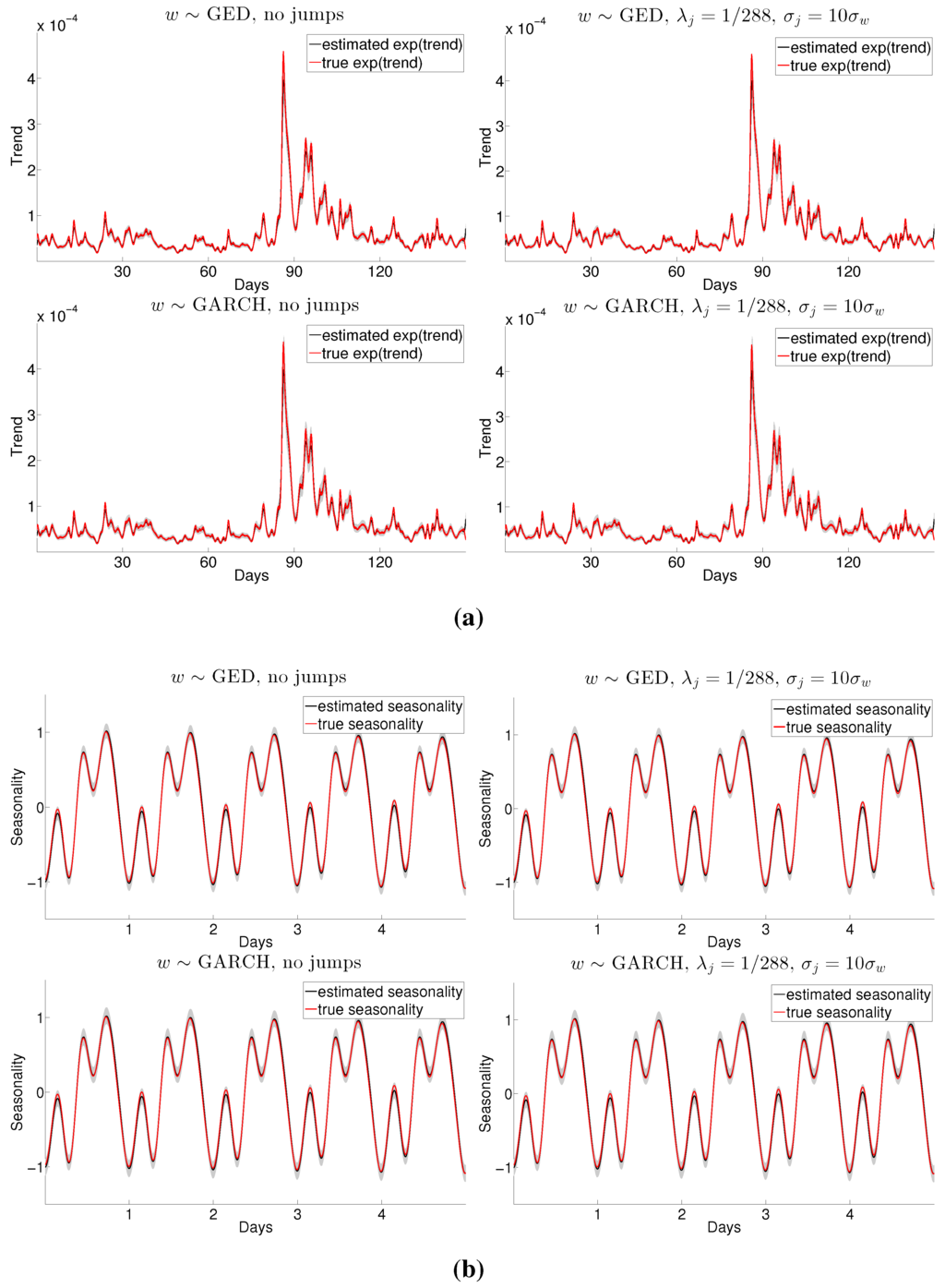
Figure 1.
Trend and seasonality preliminary simulation results. In each panel: mean estimate (black line), true quantity (red line) and estimated 95% confidence intervals (shaded area). (a) Trend for the entire (simulated) data; (b) Seasonality for the first week of the (simulated) data.

Table 1.
Trend and seasonality complete simulation results. In each cell: trend (left) and seasonality (right).
| Fourier Flexible Form | GED | EGARCH(1,1) | GARCH(1,1) | |
| No jumps | AISE | |||
| AIAE | ||||
| , | AISE | |||
| AIAE | ||||
| , | AISE | |||
| AIAE | ||||
| , | AISE | |||
| AIAE | ||||
| , | AISE | |||
| AIAE | ||||
| Synchrosqueezed Transform | GED | EGARCH(1,1) | GARCH(1,1) | |
| No jumps | AISE | |||
| AIAE | ||||
| , | AISE | |||
| AIAE | ||||
| , | AISE | |||
| AIAE | ||||
| , | AISE | |||
| AIAE | ||||
| , | AISE | |||
| AIAE | ||||
4. Application to Foreign Exchange Data
As an empirical application, we study the EUR/USD, EUR/GBP, JPY/USD, and USD/CHF exchange rates from the beginning of 2010 to the end of 2013. We avoid the data preprocessing by using pre-filtered five minute bid-ask pairs obtained from Dukascopy Bank SA. 4 The log-price is computed as the average between the log-bid and log-ask prices, and the return is defined as the change between two consecutive log-prices.
Because trading activity unquestionably drops during weekends and certain holidays (see, e.g., [4,5]), we always exclude a number of days from the sample, from 21:05 GMT the night before until 21:00 GMT that evening. For instance, weekends start on Friday at 21:05 GMT and last until Sunday at 21:00 GMT. Using this definition of the trading day, we remove the fixed holidays of Christmas (24 December to 26 December) and New Year’s (31 December to 2 January), and the holidays of Martin Luther King’s Day, President’s Day, Good Friday, Memorial Day, Independence Day, Labor Day and Thanksgiving. After these exclusions, we obtain a sample of 998 days of data, containing intraday returns.
In Panel 2a of Figure 2, we show the return for the four considered exchange rates for the first week of trading, that is, from 3 January 2010 (Sunday) at 21:05 GMT to 8 January 2010 (Friday) at 21:00 GMT (1440 observations). Although heteroskedasticity is obviously present, it is arguably easier to discern its periodicity by looking at the log-volatility in Panel 2b. Note that the smallest observations correspond to the case in which the price does not move during the five-minutes interval (i.e., and ).
In Figure 3, the autocorrelation (Panel 3a) and the power spectrum (Panel 3b) of the log-volatility indicate strong (daily) periodicities in the log-volatility. Although the shapes are different for the various exchange rates, they all essentially display the same information; on average, the seasonality is composed of periodic components of integer frequency. Note that “on average” emphasizes that both representations are only part of the picture. As illustrated in Section 2.4, this representation misses the dynamics of the signal: for example, some of the underlying periodic components may strengthen, weaken, or completely disappear at some point. Another observation is that the JPY/USD curves are fairly different from the others. First, according to the autocorrelation, the overall magnitude of oscillations (i.e., the importance of the daily periodicity) is smaller. Second, according to the height of the power spectrum’s second peak, the amplitude of the second component is much larger.
In Figure 4, Figure 5 and Figure 6, we show the reconstruction results and compare them to more traditional estimators. For the trend, is estimated using (18) with a frequency threshold of daily oscillations and an upper integration bound corresponding to the highest frequency that can be resolved according to the Nyquist theorem (i.e., half of the sampling frequency ). It is compared to the realized volatility (RV) and bipower variation (BV, see [27]), which are computed as rolling moving averages of and , with 288 and 287 observations included (except near the borders) and maximal overlap. For the seasonality, we use the synchrosqueezing transform (SST) to estimate by (16) and (17), and . The Fourier flexible form or rolling Fourier flexible form (FFF or rFFF) are estimated using the ordinary least-square estimator on the entire sample or a four-weeks rolling window. To obtain confidence intervals, we apply the following procedure:
- Use and to recover for .
- Bootstrap B samples for and .
- Add back and to in order to obtain for and .
- Estimate and for and to compute pointwise confidence intervals.
As are found to be autocorrelated, a naive bootstrapping scheme is not appropriate. To deal with this dependence issue, we use the automatic block-length selection procedure from [28], along with circular block-bootstrap. The pointwise bootstrapped distribution of the estimates is found to be approximately normal. However, a bias correction proves to be necessary, which is achieved for the trend by substracting the bootstrapped bias from the estimate .
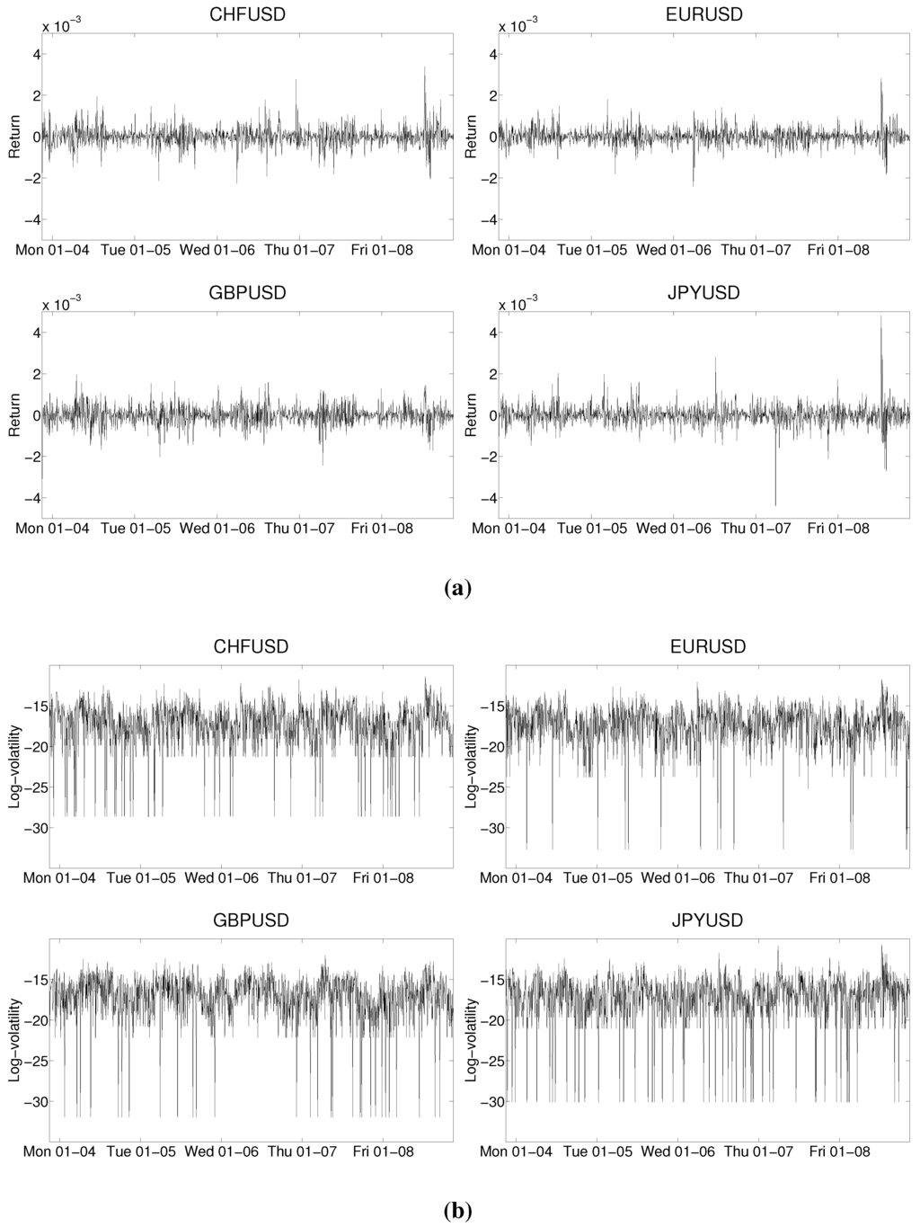
Figure 2.
First week of returns and log-volatilities in January 2010. Top: CHF/USD (left) and EUR/USD (right); Bottom: GBP/USD (left) and JPY/USD (right). (a) Return ; (b) Log-volatility .
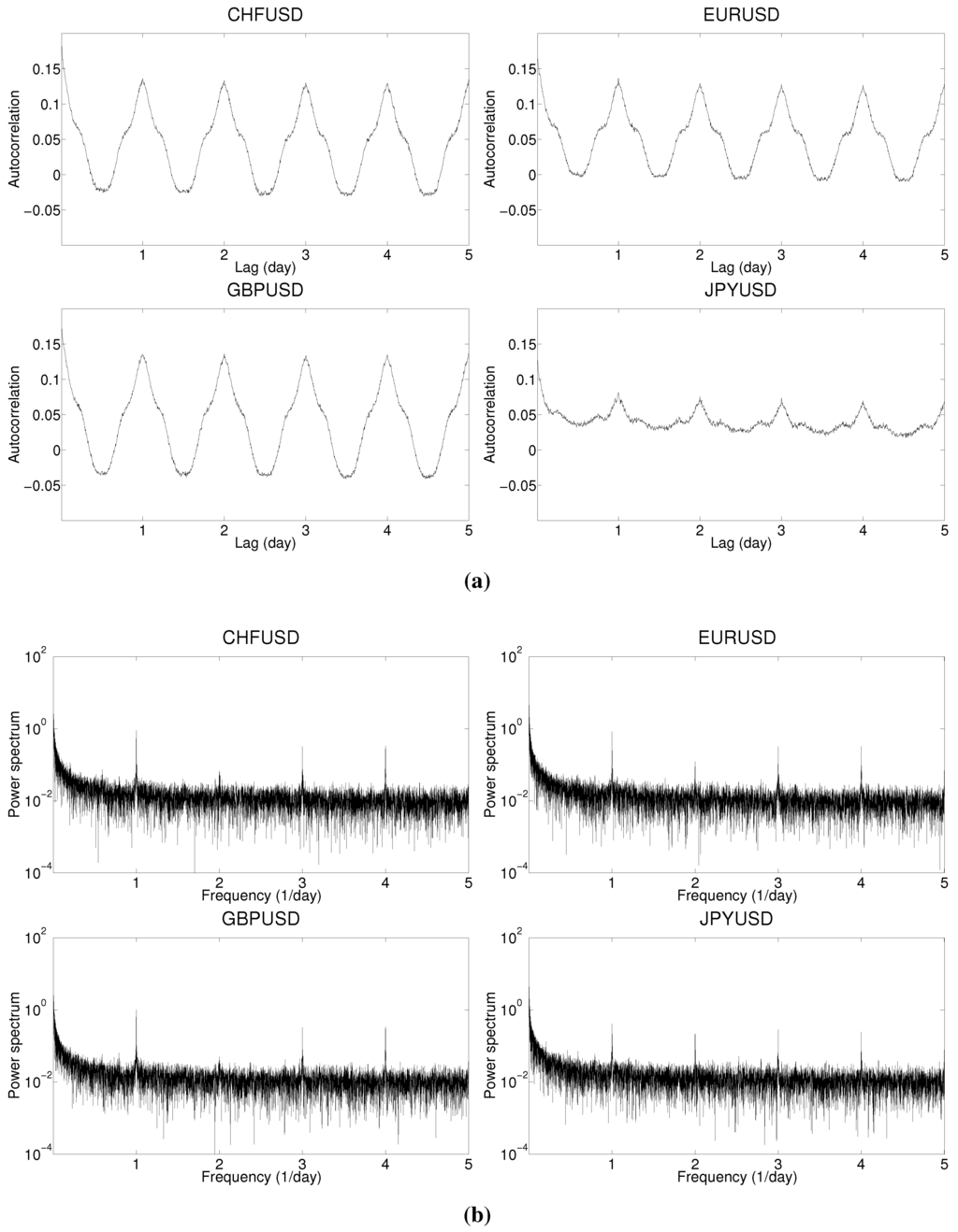
Figure 3.
Autocorrelation and power spectrum of the log-volatility. and . Top: CHF/USD (left) and EUR/USD (right); Bottom: GBP/USD (left) and JPY/USD (right). (a) Autocorrelation . The lag l is from 1 to 1440 and the x axis ticks are divided by 288; (b) Power spectrum . The frequency ω is from 0 to 5.
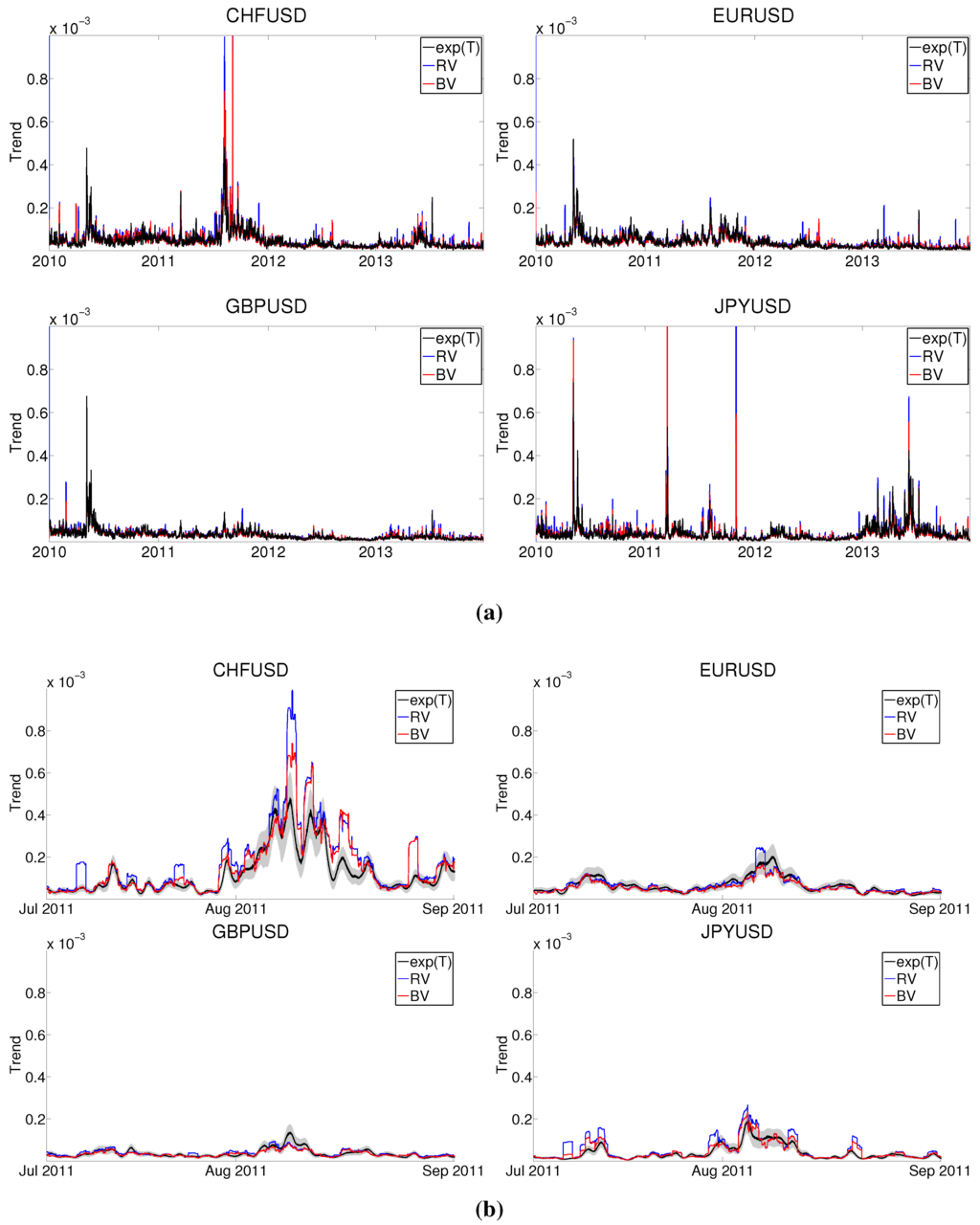
Figure 4.
Trend reconstruction results. In each panel: reconstructed trend (black line), realized volatility (red line) and bipower variation (blue line). In Panel 4b: 95% confidence intervals for the reconstructed trend (shaded area). Top: CHF/USD (left) and EUR/USD (right); Bottom: GBP/USD (left) and JPY/USD (right). (a) Trend reconstruction for 2010–2013; (b) Zoom during the summer of 2011.
The results are separately presented for the trend in Figure 4 and for the seasonality in Figure 5 and Figure 6. In Panel 4a, our reconstructed trend is compared to the realized volatility and bipower variation for the 2010–2013 period. The estimates are only represented between 0 and for the sake of visual clarity, and a few jumps in the CHF/USD and JPY/USD exchange rates generate peaks well above the upper limit. In Panel 4b, the three trend estimates are compared over a shorter time period in the summer of 2011, in the middle of United States debt-ceiling crisis and European sovereign debt crisis of 2011. Our reconstructed trend visibly constitutes a smoothed version of the usual volatility measures, which generally fall inside of the 95% confidence interval except for upward spikes due to jumps. Notice the steep volatility increase in all exchange rates as stock markets around the world started to fall, following the downgrading of United States’ credit rating on 6 August 2011 by Standard & Poor’s. This is especially true for the Swiss franc, which encountered increasing pressure from currency markets because it is considered a safe investment in times of economic uncertainty.
In Figure 5, we show the amplitude modulations of the first periodic component. When a unique Fourier flexible form is estimated for the whole sample, the corresponding amplitude is very close to the mean amplitude obtained with the synchrosqueezing transform. We observe that the rolling Fourier flexible form closely tracks the synchrosqueezing transform, but is far wigglier. This was expected because the synchrosqueezing transform estimator is essentially an instantaneous (and smooth by construction) version of the Fourier flexible form. As expected from Figure 3, the amplitude modulations of the first component in the JPY/USD are much smaller than the three other exchange rates.
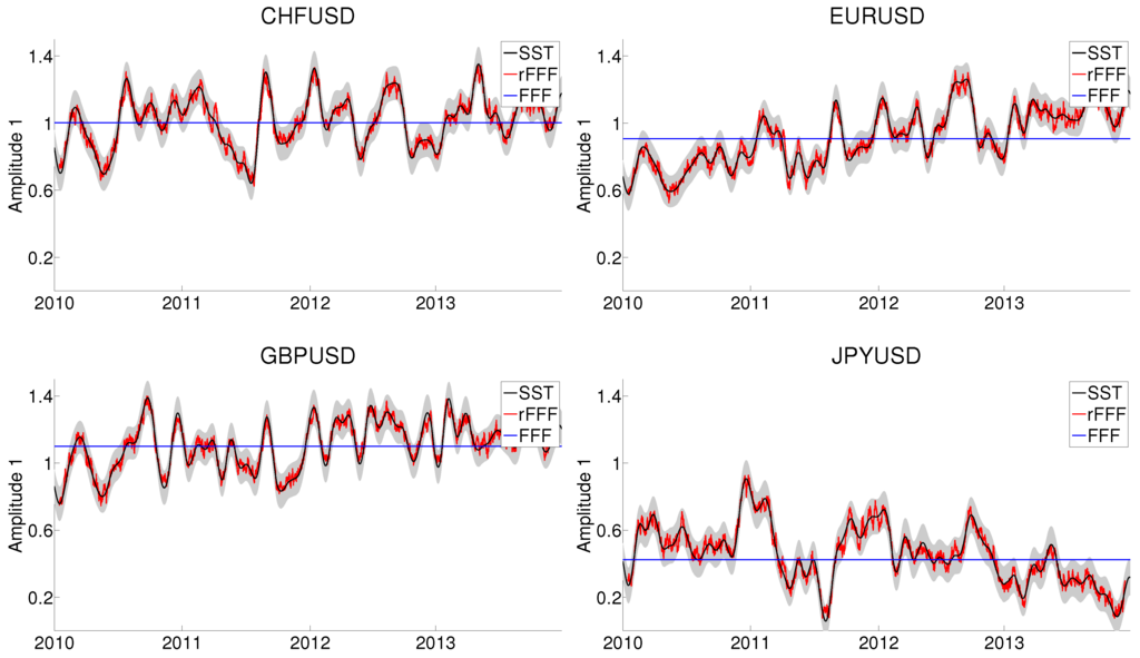
Figure 5.
Amplitude modulations reconstruction results. In each panel: reconstructed amplitude modulations of the first component (black line) with 95% confidence intervals (shaded area), Fourier flexible form (dashed line) and rolling Fourier flexible form (red line). (Top) CHF/USD (left) and EUR/USD (right); (Bottom) GBP/USD (left) and JPY/USD (right).
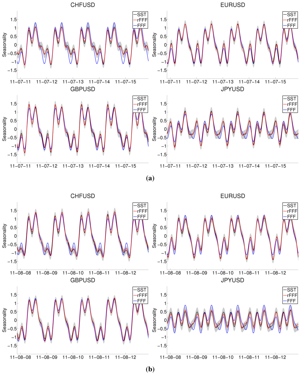
Figure 6.
Seasonality reconstruction results. In each panel: reconstructed seasonality (black line) with 95% confidence intervals (shaded area) and rolling Fourier flexible form (red line). Top: CHF/USD (left) and EUR/USD (right); Bottom: GBP/USD (left) and JPY/USD (right). (a) Second week of July 2011; (b) Second week of August 2011.
In Panels 6a and 6b of Figure 6, we show the seasonality estimated as a sum of the four periodic components: the Fourier flexible form represents the average daily oscillation, the rolling Fourier flexible form is a wiggly estimate of the dynamics, and the synchrosqueezing transform extracts a smooth instantaneous seasonality. As in Figure 5, we observe that the overall magnitude of oscillation is much smaller in the JPY/USD exchange rate.
In summary, a striking feature of our estimated trend is its robustness to jumps, which affect both the realized volatility and, albeit to a lesser extent, the bipower variation. Figure 5 and Figure 6 strongly suggest that the seasonality evolves dynamically over time. Although similar estimates of trend and seasonality can be obtained with moving averages and rolling regressions respectively, the synchrosqueezing transform provides smooth estimates and does not require an arbitrary choice of the length of the window or the rolling overlap. One could argue that the choice of a mother wavelet is also arbitrary, the influence of this choice on the synchrosqueezing transform estimators is negligible (see [22,25]). In any case, the main message is that dynamic methods are necessary to properly understand the seasonality, as static models can lead to severe underestimation or overestimation of the intraday spot volatility.
5. Discussion
Our disentangling of instantaneous trend and seasonality of the intraday spot volatility is an extension of classical econometric models that provides adaptivity to ever-changing markets. The proposed method suggests a realistic framework for the high-frequency time series behavior. First, the method allows the daily component of the volatility to be modeled as an instantaneous trend evolving in real time within the day. Second, the model allows the seasonality to be non-constant over the sample. In a simulation study using a realistic setting, numerical results confirm that the proposed estimators for the trend and seasonality components behave appropriately. We show that this result holds even in the presence of heteroskedastic and heavy-tailed noise, and it is robust to jumps.
Using the CHF/USD, EUR/USD, GBP/USD, and USD/JPY exchange rates sampled every fite minutes between 2010 and 2013, we confirm empirically that the oscillation frequency is constant, as originally suggested in the Fourier flexible form from [3,4]. In the four exchange rates, we show that the amplitude modulations of the periodic components, and hence the overall magnitude of oscillation, evolve dynamically over time. As such, neglecting those modulations in the periodic part of the volatility would imply either an overestimation (when the periodic components are lower than their mean value), or an underestimation (when the periodic components are higher than their mean value). We show that the synchrosqueezing transform estimator produces results comparable to a smooth version of a rolling Fourier flexible form. However, the adaptivity of synchrosqueezing transform should still be emphasized, because it does not require ad-hoc choices for the rolling overlapping ratio or of the length of each window, as for a parametric regression.
Although we illustrate our model by simultaneously disentangling the low- and high-frequency components of the intraday spot volatility in the foreign exchange market, it is possible to embed the new methodology into a forecasting exercise. This exercise may be useful in the context of an investor’s optimal portfolio choice or for risk-management purposes, which is beyond the scope of this paper’s aim of presenting the modeling framework. Further research directions include the extension of the framework to the multivariate data and the non-homogeneously sampled (“tick-by-tick”) data. We will return to these questions and related issues in future works.
Acknowledgments
Most of this research was conducted while the corresponding author was visiting the Berkeley Statistics Department. He is grateful for its support and helpful discussions with the members both in Bin Yu’s research group and the Coleman Fung Risk Management Research Center. This research is also supported in part by the Center for Science of Information (CSoI), a US NSF Science and Technology Center, under grant agreement CCF-0939370, and by NSF grants DMS-1160319 and CDS&E-MSS 1228246.
Author Contributions
Thibault Vatter and Hau-Tieng Wu conceived and developed the methodology. Hau-Tieng Wu contributed the theoretical aspects and the legacy code to perform a Synchrosqueezing Transform. Thibault Vatter adapted the code to the financial context and analyzed the data. Valérie Chavez-Demoulin and Bin Yu supervised the project and contributed to the writing.
Conflicts of Interest
The authors declare no conflict of interest.
Appendix. Implementation Details
In this section, we provide the numerical synchrosqueezing form implementation details. The MATLAB code is available from the authors upon request, and we refer the readers to [29] for more implementation details.
We fix a discretely sampled time series , where , with τ as the sampling interval and for . Note that we use the bold notation to indicate the numerical implementation (or the discrete sampling) of an otherwise continuous quantity.
Step 1: numerically implement .
We discretize the scale axis a by , , where is the voice number chosen by the user. In practice, we choose . We denote the numerical continous wavelet transform as a matrix . This is a well-studied step, and our continous wavelet transform implementation is modified from that of wavelab5.
Step 2: numerically implement .
The next step is to calculate the instantaneous frequency information function (14). The term is implemented directly by finite difference at t axis, and we denote the result as an matrix . The is implemented as an matrix by the following entry-wise calculation:
where NaN is the IEEE arithmetic representation for Not-a-Number.
Step 3: numerically implement .
We now compute the synchrosqueezing transform (15). We discretize the frequency domain by equally spaced intervals of length . Here and are the minimal and maximal frequencies detectable by the Fourier transform theorem. Denote , which is the number of the discretization of the frequency axis. Fix , is discretized as an matrix by the following evaluation
where and . Notice that the number γ is a hard thresholding parameter, which is chosen to reduce the influence of noise and numerical error. In practice, we simply choose γ as the quantile of . If the error is Gaussian white noise, the choice of γ is suggested in [29]. In general, determining how to adaptively choose γ is an open problem.
Step 4: estimate the instantaneous frequency, amplitude modulation and trend from .
We fit a discretized curve , where is the index set of the discretized frequency axis, to the dominant area of , by maximizing the following functional over :
where . The first term is used to capture the maximal value of at each time, and the second term is used to impose regularity on the extracted curve. In other words, the user-defined parameter λ determines the smoothness of the resulting curve estimate. In practice, we simply choose . Denote the maximizer of the functional as . In that case, the estimator of the IF of the k-th component at time is defined as
where . With , the k-th component and its amplitude modulation, at time are estimated by:
where ℜ is the real part, , and . Lastly, we estimate the trend at time by
where and is determined by the model.
References
- T.G. Andersen, T. Bollerslev, F.X. Diebold, and P. Labys. “Modeling and Forecasting Realized Volatility.” Econometrica 71 (2003): 579–625. [Google Scholar] [CrossRef]
- D.M. Guillaume, O.V. Pictet, and M.M. Dacorogna. On the intra-daily performance of GARCH processes, Working papers. Zurich, Switzerland: Olsen and Associates, 1994. [Google Scholar]
- T.G. Andersen, and T. Bollerslev. “Intraday periodicity and volatility persistence in financial markets.” J. Empir. Financ. 4 (1997): 115–158. [Google Scholar] [CrossRef]
- T.G. Andersen, and T. Bollerslev. “Deutsche Mark–Dollar Volatility : Intraday Activity Patterns, Macroeconomic Announcements, and Longer Run Dependencies.” J. Financ. 53 (1998): 219–265. [Google Scholar] [CrossRef]
- M.M. Dacorogna, U.A. Müller, R.J. Nagler, R.B. Olsen, and O.V. Pictet. “A geographical model for the daily and weekly seasonal volatility in the foreign exchange market.” J. Int. Money Financ. 12 (1993): 413–438. [Google Scholar] [CrossRef]
- R. Gencay, M. Dacorogna, U.A. Muller, O. Pictet, and R. Olsen. An introduction to high-frequency finance. Waltham, MA, USA: Academic press, 2001. [Google Scholar]
- T. Bollerslev, and E. Ghysels. “Periodic autoregressive conditional heteroscedasticity.” J. Bus. Econ. Stat. 14 (1996): 139–151. [Google Scholar]
- K. Boudt, C. Croux, and S. Laurent. “Robust estimation of intraweek periodicity in volatility and jump detection.” J. Empir. Financ. 18 (2011): 353–367. [Google Scholar] [CrossRef]
- H.G. Müller, R. Sen, and U. Stadtmüller. “Functional data analysis for volatility.” J. Econom. 165 (2011): 233–245. [Google Scholar] [CrossRef]
- R.F. Engle, and M.E. Sokalska. “Forecasting intraday volatility in the US equity market. Multiplicative component GARCH.” J. Financ. Econom. 10 (2012): 54–83. [Google Scholar] [CrossRef]
- W.K. Newey, and D. McFadden. “Large sample estimation and hypothesis testing.” In Handbook of Econometrics. Edited by R.F. Engle and D.L. McFadden. Philadelphia, PA, USA: Elsevier, 1994, Volume 4, pp. 2111–2245. [Google Scholar]
- M. Martens, Y.C. Chang, and S.J. Taylor. “A comparison of seasonal adjustment methods when forecasting intraday volatility.” J. Financ. Res. 25 (2002): 283–299. [Google Scholar] [CrossRef]
- P. Giot. “Market risk models for intraday data.” Eur. J. Financ. 11 (2005): 309–324. [Google Scholar] [CrossRef]
- R. Gallant. “On the bias in flexible functional forms and an essentially unbiased form: The fourier flexible form.” J. Econom. 15 (1981): 211–245. [Google Scholar] [CrossRef]
- R. Deo, C. Hurvich, and Y. Lu. “Forecasting realized volatility using a long-memory stochastic volatility model: Estimation, prediction and seasonal adjustment.” J. Econom. 131 (2006): 29–58. [Google Scholar] [CrossRef]
- H. Laakkonen. Exchange rate volatility, macro announcements and the choice of intraday seasonality filtering method. Research Discussion Papers 23/2007; Helsinki, Finland: Bank of Finland, 2007. [Google Scholar]
- A. Beltratti, and C. Morana. “Deterministic and Stochastic Methods for Estimation of Intraday Seasonal Components with High Frequency Data.” Econ. notes 30 (2001): 205–234. [Google Scholar] [CrossRef]
- I. Daubechies. Ten Lectures on Wavelets. Philadelphia, PA, USA: SIAM: Society for Industrial and Applied Mathematics, 1992. [Google Scholar]
- P. Flandrin. Time-frequency/time-scale Analysis, Wavelet Analysis and Its Applications. Waltham, MA, USA: Academic Press Inc., 1999. [Google Scholar]
- J.C. Cox, J.E. Ingersoll Jr., and S.A. Ross. “A Theory of the Term Structure of Interest Rates.” Econometrica 53 (1985): 385–407. [Google Scholar] [CrossRef]
- S.L. Heston. “A closed-form solution for options with stochastic volatility with applications to bond and currency options.” Rev. Financ. Stud. 6 (1993): 327–343. [Google Scholar] [CrossRef]
- Y.C. Chen, M.Y. Cheng, and H.T. Wu. “Non-parametric and adaptive modelling of dynamic periodicity and trend with heteroscedastic and dependent errors.” J. R. Stat. Soc.: Ser. B (Stat. Methodol.) 76 (2014): 651–682. [Google Scholar] [CrossRef]
- C.M. Hafner, and O. Linton. “An Almost Closed form Estimator for the EGARCH Model.” Available online: http://ssrn.com/abstract=2139516 (accessed on 19 August 2015).
- D.B. Nelson. “Conditional heteroskedasticity in asset returns a new approach.” Econometrica 29 (1991): 347–370. [Google Scholar] [CrossRef]
- I. Daubechies, J. Lu, and H.T. Wu. “Synchrosqueezed wavelet transforms: An empirical mode decomposition-like tool.” Appl. Comput. Harmon. Anal. 30 (2011): 243–261. [Google Scholar] [CrossRef]
- I. Daubechies, and S. Maes. “A nonlinear squeezing of the continuous wavelet transform based on auditory nerve models.” In Wavelets in Medicine and Biology. Boca Raton, FL, USA: CRC-Press, 1996, pp. 527–546. [Google Scholar]
- O.E. Barndorff-Nielsen. “Power and Bipower Variation with Stochastic Volatility and Jumps.” J. Financ. Econom. 2 (2004): 1–37. [Google Scholar] [CrossRef]
- D.N. Politis, and H. White. “Automatic Block-Length Selection for the Dependent Bootstrap.” Econom. Rev. 23 (2004): 53–70. [Google Scholar] [CrossRef]
- G. Thakur, E. Brevdo, N.S. Fuckar, and H.T. Wu. “The Synchrosqueezing algorithm for time-varying spectral analysis: Robustness properties and new paleoclimate applications.” Signal Process. 93 (2013): 1079–1094. [Google Scholar] [CrossRef]
- 1[3,4] consider the addition of dummy variables to capture weekday effects or particular events such as holidays in particular markets, in addition to unemployment reports, retail sales figures, etc. While the periodic model captures most of the seasonal patterns, their dummy variables allow the quantification of the relative importance of calendar effects and announcement events.
- 2 and for all , and so that for all and
- 3Although not reported here, the pointwise biases and variances for the trend and seasonality were also studied. While the biases are again indistinguishable (and basically negligible for the trend) between the GED or GARCH with or without jumps, the variances are higher for the GARCH, and show no visible from the jumps.
© 2015 by the authors; licensee MDPI, Basel, Switzerland. This article is an open access article distributed under the terms and conditions of the Creative Commons Attribution license ( http://creativecommons.org/licenses/by/4.0/).