1. Introduction
Kwiatkowski
et al. (KPSS) [
1] have proposed an LM test with a null hypothesis such that a series is level or trend stationary and these authors assigned the limit theory under the null. By the same token, these researchers have also analyzed the test’s asymptotic power under the difference stationarity alternative. At present, the KPSS test is widely used in empirical studies to examine trend stationarity. This test is used as a complement to the standard unit root tests in analyzing time series properties. In addition, the asymptotic distribution of the KPSS test depends on whether the data are filtered by a preliminary regression. Specifically, if a mean or linear trend is extracted, then the asymptotic distribution of the test statistic changes, and its critical values should be adequately adjusted. This approach to testing unit roots by reversing the null and alternative hypotheses encouraged several statisticians and econometricians to establish other generalizations.
There have been several studies in favor of seasonal adjustment encountered in the literature; see,
inter alia, [
2,
3,
4]. To support this adjustment line of thinking, there are also several arguments. First, seasonal adjustment may provide better results in terms of forecasting. Second, seasonality can hide slight changes in trends; therefore, comparing between two economic series is more complicated. Nevertheless, the use of seasonally unadjusted data is currently on the rise. This finding can be interpreted, in large part, by the fact that inference distortion and detrimental information loss in dynamic models could result from seasonal adjustment. Moreover, several authors have demonstrated that the seasonal and cyclical components are linked, unlike the traditional statistical view, which states that the business and seasonal cycles are phenomena to be studied separately; see,
inter alia, [
5,
6,
7]. In this way, the systematic elimination of the seasonal component may generate questionable deductions. However, having decided not to eliminate this component, the following question can be immediately raised: What model should be given to seasonality?
As an answer to the above question, the literature has considered three widely used approaches for modeling seasonality: Deterministic seasonal processes and stationary and non-stationary processes. Dickey, Hasza and Fuller [
8] are among the first authors to introduce a seasonal unit root test through the generalization of the Dickey-Fuller unit root test for seasonal data. However, the test by Hylleberg
et al. [
9] is now the preeminent seasonal unit root test, with its asymptotic orthogonality being a key property, allowing for generalizations at any observational frequency. The subsequent rejection of their null hypothesis implies a strong result that the series exhibits a stationary seasonal pattern. It would be useful to note that the test by Hylleberg
et al. [
9] was originally introduced for quarterly data. For that reason, several authors have generalized this test to other observational frequencies. In this regard, one can quote the extension of Beaulieu and Miron [
10] to monthly data. However, the test by Hylleberg
et al. [
9] is found to suffer from the problem of low power in moderate sample sizes. In agreement with what was found in the conventional case, Hylleberg [
11] suggested the joint use of the seasonal unit root and stationarity tests. The treatment of the seasonal variable should be performed with caution. On the one hand, and as shown by Franses
et al. [
12], considering seasonality as deterministic while the data actually exhibits seasonal unit roots may ultimately result in a spurious regression. Indeed, the corresponding coefficient of determination
of a regression of a first-order differenced time series on seasonal dummy variables is not, in this case, a reliable measure of the amount of seasonal fluctuations that can be explained by a deterministic variation in the series. On the other hand, and as was mentioned by Demetrescu and Hassler [
13], the result obtained by Franses
et al. [
12] may not lead to neglecting deterministic seasonality because it may capture primarily reality on occasion.
The literature is relatively sparse in regards to seasonal stationarity tests. Canova and Hansen [
14] and Caner [
15] are among the first authors to develop tests in this category. The difference between the two tests lies in the correction of the error term when the standard assumptions do not apply. In other words, the first test used a non-parametric correction, as in the KPSS test, and the second used a parametric correction. Likewise, Lyhagen [
16] proposed another version of the KPSS test in the seasonal context which resulted in a frequency-based test. In particular, Lyhagen [
16] tested the null hypothesis of level stationarity against a single seasonal unit root. Thus, this test can be termed the seasonal KPSS test.
Khédhiri and El Montasser [
17] used a Monte Carlo method to demonstrate that the seasonal KPSS test is robust to the magnitude and number of additive outliers. Furthermore, the obtained statistical results cast an overall good performance of the finite-sample properties of the test. Khédhiri and El Montasser [
18] have provided a representation of the seasonal KPSS test in the time domain and established its asymptotic theory. This representation enables the generalization of the test’s asymptotic theory when the basic equation incorporates other additional dynamics. However, Khédhiri and El Montasser [
18], similar to Lyhagen [
16], have taken into account only quarterly data. In their studies, the deterministic component is reduced to only seasonal dummy variables. The purpose of this paper is to overcome this limitation. To this end, other observational frequencies are considered in this study by examining monthly data. Similarly, the effect of the presence of a linear trend on the seasonal KPSS test in finite samples for quarterly and monthly data is considered. In addition, a sketch of the test’s asymptotic theory is provided in the presence of a linear trend.
The paper is structured as follows. In
Section 2, several preliminaries of the seasonal KPSS are introduced. In
Section 3, a Monte Carlo simulation study is conducted to assess the finite sample properties of the test in terms of its size and power performance when including a linear trend in its basic equations. Moreover, the effect of the observational frequency on the test properties is considered in this study. To this end, monthly and quarterly data are studied together.
Section 4 provides an application of the seasonal KPSS test.
Section 5 presents the conclusions.
2. Preliminaries on the Seasonal KPSS Test
Let be a time series observed quarterly. Because the goal is to test for the presence of a negative unit root, it would be suitable to use the appropriate filter to isolate the effects of other unit roots in the series. Therefore, the test will be applied to the transformed series: where is the lag operator. This transformation is obtained from the seasonal difference filter
Next, one tests the unit root of −1 in the series
where
and
with the shorthand notation
and also (.) denotes the largest integer function and
is the Kronecker
function.
The term is a zero mean weakly dependent process with autocovariogram and a strictly positive long run variance .
The component
is drawn from the following process:
where
is a zero mean weakly process with variance
and a long run variance
.
The transformation needed to run the seasonal KPSS test for complex unit roots is given by the following variable, .
The test of such complex unit roots is based on the regression,
where
is a zero mean weakly dependent process with a long run variance
and
. The component
is given by
where
is another zero mean weakly dependent process with variance
and a strictly positive long run variance
.
Adding the deterministic terms in Equations (1) and (3) is highly important because it allows the seasonal KPSS test to include deterministic seasonality. The testing procedure is performed in two steps: First, the unit root of −1 is tested, and the complex roots subsequently are tested (their null hypothesis will be specified thereafter).
The seasonal KPSS test is a Lagrange Multiplier-based test. Hence, the null hypothesis of a root that is equal to −1 is
. Under this null hypothesis,
is written as:
where the series is trend stationary after seasonal mean correction. Under the alternative hypothesis
has a unit root corresponding to the Nyquist frequency.
Let
be the residual series obtained from a least squares regression applied to Equation (5),
. Following Breitung and Franses [
19] (Equation (18), p. 209), Busetti and Harvey [
20] (Equation (8), p. 422) and Taylor [
21] (Equation (38), p. 605), we replace the long-run variance
with an estimate of (
times) the spectrum at the observed frequency to address unconditional heteroskedasticity and serial correlation. This nonparametric estimation of the long-run variance is a useful solution to the
nuisance parameter problem [21]. Thus, for the Nyquist frequency, this nonparametric estimation is written as follows:
where the weight function
and
is a lag truncation parameter such that
as
and
A Bartlett kernel, following Newey and West [
22], is chosen in line with Andrews [
23], who has shown that such a truncation lag can produce good results in practice, as also shown in [
1]. Similarly, the null hypothesis of the test regarding complex unit roots is given by
. Under this null hypothesis,
is written as follows:
Using the residuals
obtained from the least squares regression of Equation (7), the Bartlett kernel estimator of
can be computed as follows:
Define the partial sums and .
It follows that the test statistic for the unit root of −1 is given by:
This statistic may be written for the complex unit roots, as
where
and
are the conjugate numbers of
and
, respectively.
Khédhiri and El Montasser [
18] have shown that under
,
where
is a standard Brownian bridge, “
” denotes weak convergence in probability and
. However, for
, the authors have shown that
where
and
are two independent standard Brownian bridges and
.
Remark 1: Asymptotically
has, in Harvey’s [
24] terminology, the first level Cramer-von Mises distribution (
) under the null hypothesis while the limit theory of
was shown to be a function of a generalized Cramer-von Mises with two degrees of freedom. Specifically, the asymptotic theory of this statistic is as follows:
The reader can refer to Anderson and Darling [
25] for a discussion of this type of distribution. The critical values of the seasonal KPSS test with seasonal dummies can be computed from Nyblom [
26] or from Canova and Hansen [
14]. These critical values are also shown in
Table 1 of Khédhiri and El Montasser [
18].
Table 1.
Critical values of the seasonal KPSS test in the case of a first order polynomial trend.
Table 1.
Critical values of the seasonal KPSS test in the case of a first order polynomial trend.
| Unit roots | 1% | 5% | 10% |
|---|
| −1 | 2.787 | 1.656 | 1.196 |
| 1.9645 | 1.3120 | 1.031 |
Remark 2: It can be shown that the seasonal frequency has no effect on the asymptotic distribution of test statistics. In other words, may retain the same limit distribution as above and the statistic associated with the complex unit roots in question has the same limit distribution as . Only the set of seasonal unit roots change, and it may not include the unit root that corresponds to the Nyquist frequency, i.e., when the periodicity is odd.
Remark 3: Recall that if there is a time trend in the regression of the standard KPSS test, the partial sum of residuals from a first order polynomial regression weakly converges to a second level Brownian bridge, denoted as
, where, as in MacNeill [
27],
with
being a standard Wiener process or a Brownian motion.
Then, the test statistic follows the so-called second level Cramer von Mises distribution; see [
24]. However, this result cannot be generalized to the seasonal KPSS test. More specifically, the statistic
follows the so called zero level Cramer von Mises, denoted as
; see [
24]. Specifically,
Meanwhile, when the deterministic component is represented by only a trend in Equation (3), it can be shown that
The critical values of the seasonal KPSS test in this case can be obtained from Nyblom [
26] (
Table 1) and they are shown in
Table 1. Even though only a constant is included in Equations (1) and (3), these critical values are still appropriate. Indeed, these findings show that the generalization of the asymptotic results of the standard KPSS test should not be performed in an automatic way, but rather, it is advisable to conduct careful analysis to establish equivalent results for the seasonal KPSS test.
3. The Monte Carlo Analysis
To evaluate the size performance of the seasonal KPSS statistic in the presence of a first order linear trend, Monte Carlo simulation experiments are conducted with seasonal roots corresponding to quarterly processes. The data generating process (DGP) for the negative unit root is
where
and the autoregressive process
is given by:
The error terms are normally distributed with zero mean and unit variance.
The DGP for complex unit roots is given by
where
only includes a first order linear trend and the process
is given by:
are normally distributed with zero mean and unit variance.
The alternative values of the autoregressive coefficients are chosen so that and only the 5% nominal size is considered. The bandwidth values chosen in our experiments are given by: , integer andinteger .
This study totaled 20,000 replications and all the simulation experiments were carried out with Matlab programs. The corresponding results are summarized in
Table 2.
Table 2 reports similar findings obtained elsewhere in the literature. Indeed, the test’s size increases with decreasing values of
. Similarly, the sample size does not noticeably affect the test’s size, which means that the non-parametric corrections
and
have not been markedly taken up.
To see the effect of observational frequency on the seasonal KPSS test in finite samples, monthly periodicity is considered. In this case, the deterministic component is represented by 12 seasonal dummy variables. Remember that seasonal unit roots are exhibited by the filter
corresponding to the seasonal frequencies
For size experiments, a particular value of the null hypothesis is considered so that an i.i.d. process is specified as a data generating process. For power experiments, the process
, for seasonal frequencies other than the Nyquist one, is outlined by
However, when the process shows a unit root corresponding to the Nyquist frequency,
will be generated by
The considered sample sizes are T = 240 and T = 600, which display, respectively, numbers of 20 and 50 years. Both values are met in Monte Carlo studies regarding seasonal unit root tests; see,
inter alia, [
8]. As mentioned above, the critical values of the test are obtained from
Table 1 of Khédhiri and El Montasser [
18] where the first line corresponds to the unit root −1 and the second to complex unit roots.
Table 2.
Rejection frequencies for the seasonal KPSS test with a first order polynomial trend for seasonal quarterly unit roots, significance level: 5% (size and power).
Table 2.
Rejection frequencies for the seasonal KPSS test with a first order polynomial trend for seasonal quarterly unit roots, significance level: 5% (size and power).
| |
|---|
| T | | | | | | |
|---|
| −1 | 80 | 0.9492 | 0.7218 | 0.2127 | 0.9774 | 0.9092 | 0.3863 |
| 200 | 0.9936 | 0.8498 | 0.5981 | 0.9987 | 0.9734 | 0.8138 |
| 500 | 0.9999 | 0.9563 | 0.7893 | 1 | 0.9984 | 0.9489 |
| −0.9 | 80 | 0.7894 | 0.4153 | 0.1103 | 0.9123 | 0.7575 | 0.2929 |
| 200 | 0.8398 | 0.5981 | 0.1481 | 0.9627 | 0.7694 | 0.3841 |
| 500 | 0.8559 | 0.3595 | 0.1442 | 0.9770 | 0.7592 | 0.3701 |
| −0.2 | 80 | 0.1146 | 0.0534 | 0.0210 | 0.1368 | 0.0786 | 0.0243 |
| 200 | 0.1158 | 0.0577 | 0.0398 | 0.1461 | 0.0761 | 0.0403 |
| 500 | 0.1156 | 0.0570 | 0.0454 | 0.1452 | 0.0752 | 0.0505 |
| 0 | 80 | 0.0514 | 0.0398 | 0.0176 | 0.0510 | 0.0398 | 0.0173 |
| 200 | 0.0522 | 0.0473 | 0.0369 | 0.0479 | 0.0435 | 0.0331 |
| 500 | 0.0503 | 0.0469 | 0.0423 | 0.0507 | 0.0488 | 0.0435 |
| 0.2 | 80 | 0.0181 | 0.0296 | 0.0145 | 0.0126 | 0.0204 | 0.0116 |
| 200 | 0.0164 | 0.0382 | 0.0336 | 0.0100 | 0.0255 | 0.0264 |
| 500 | 0.0157 | 0.0401 | 0.0401 | 0.0104 | 0.0313 | 0.0369 |
| 0.9 | 80 | 0.0000 | 0.0053 | 0.0026 | 0.0000 | 0.0019 | 0.0007 |
| 200 | 0.0000 | 0.0006 | 0.0074 | 0.0000 | 0.0000 | 0.0007 |
| 500 | 0.0000 | 0.0075 | 0.0127 | 0.0000 | 0.0000 | 0.0006 |
In
Table 3, all empirical rejection frequencies approach the theoretical significance level of 5%. Indeed, this result shows an excellent empirical size not subject to any distortion. Moreover, an increase in sample size mostly results in a slight decrease in size.
Table 4 shows again that the seasonal KPSS test for monthly data preserves its good power properties. A reduction of power corresponding to the root of −1 and the function l12 is exceptionally notable but not surprising. Indeed, the value 0.7744 that appears in the last box of the first column of
Table 4 is very close to the values provided by [
1] (
Table 4) for the conventional unit root. This similarity is due to the mirror effect that occurs between the unit roots at frequencies of zero and
.
Table 3.
The size of the seasonal KPSS test for monthly data, significance level: 5%.
Table 3.
The size of the seasonal KPSS test for monthly data, significance level: 5%.
| Statistics | T = 240 | T = 600 |
|---|
| 0.0583 | 0.0533 |
| 0.0556 | 0.0491 |
| 0.0472 | 0.0470 |
| 0.0581 | 0.0524 |
| 0.0531 | 0.0500 |
| 0.0457 | 0.0471 |
| 0.0590 | 0.0527 |
| 0.0546 | 0.0499 |
| 0.0473 | 0.0469 |
| 0.0592 | 0.0522 |
| 0.0568 | 0.0505 |
| 0.0471 | 0.0482 |
| 0.0568 | 0.0515 |
| 0.0529 | 0.0503 |
| 0.0454 | 0.0474 |
| 0.0583 | 0.0530 |
| 0.0538 | 0.0500 |
| 0.0444 | 0.0459 |
Table 4.
The power of the seasonal KPSS test for monthly data, significance level: 5%.
Table 4.
The power of the seasonal KPSS test for monthly data, significance level: 5%.
| Statistics | T = 240 | T = 600 |
|---|
| 1 | 1 |
| 0.9988 | 0.9998 |
| 0.9493 | 0.9944 |
| 1 | 1 |
| 0.9990 | 1 |
| 0.95 | 0.9949 |
| 1 | 1 |
| 0.9987 | 1 |
| 0.9517 | 0.9943 |
| 1 | 1 |
| 0.9986 | 1 |
| 0.9515 | 0.9942 |
| 1 | 1 |
| 0.9982 | 1 |
| 0.9450 | 0.9942 |
| 1 | 1 |
| 0.9648 | 0.9929 |
| 0.7744 | 0.9194 |
4. Application
The seasonal KPSS test is applied to the monthly US consumer price index (CPI). This series covers the period from January 1913 to December 2014 and was taken from the Federal Reserve Bank of St. Louis website [
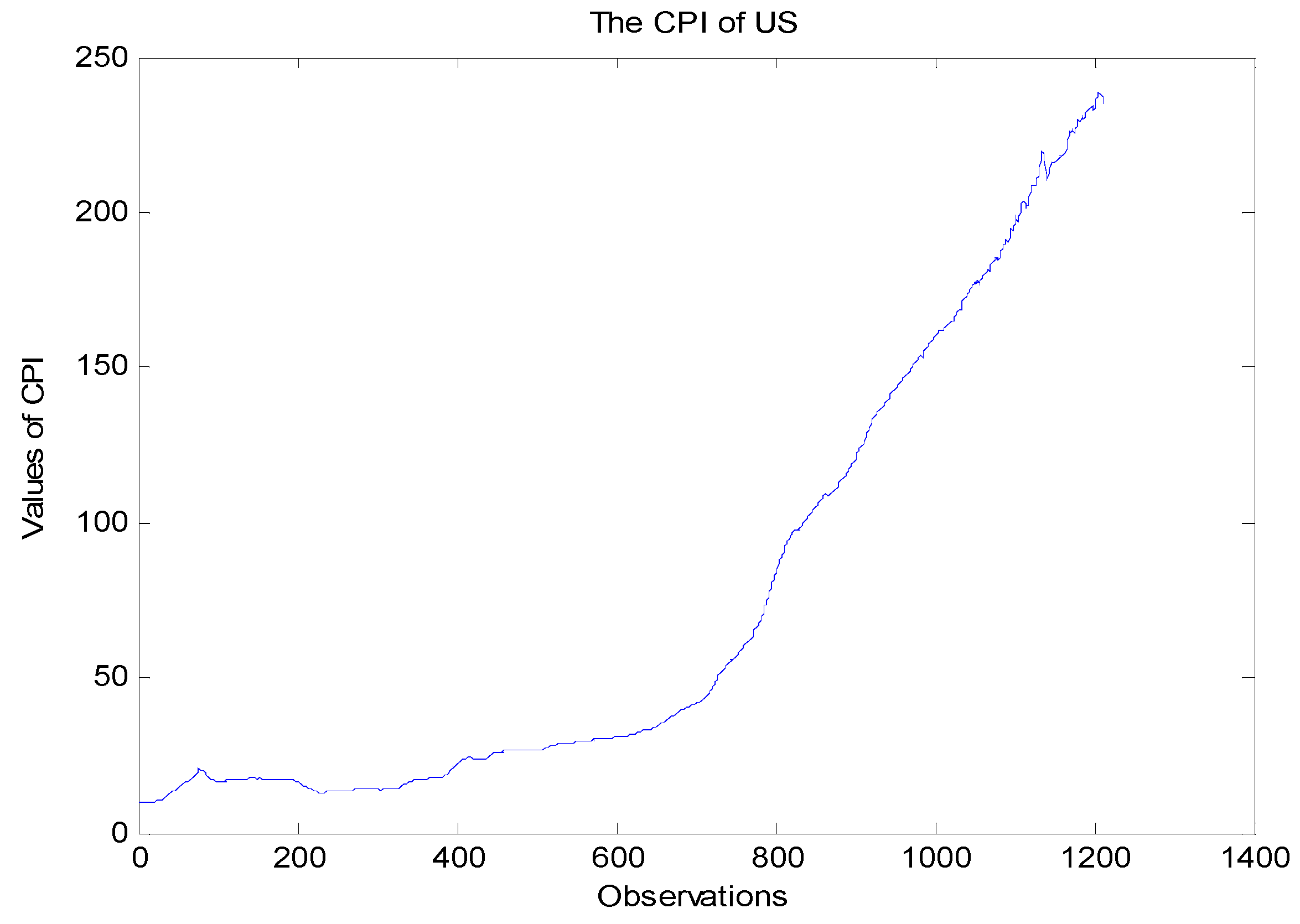
28]. The CPI shows a rising trend (see
Figure 1). This CPI series is chosen because its seasonality is recognized in the literature. In particular, Riley [
29] discussed some aspects of seasonality in the CPI. There is a variety of influences causing seasonality of consumer prices. Climatic factors are the most noteworthy, but by no means are they the only causes of periodic variations in prices. Indeed, conventions explain such variations. There are as of yet two attitudes towards seasonal variable treatment in consumer prices and, more generally, in time series. The first one considers seasonality as a serious problem for the compilation of a CPI, occurring when some of the products in the basket regularly disappear and reappear, thereby breaking the continuity of the price series from which the CPI is constructed. However, the second one admits that seasonality is not to be eliminated to better understand the series variations; see,
inter alia, [
30] who has studied the stochastic seasonality of the CPI of Turkey.
Figure 1.
The CPI of the United States.
Figure 1.
The CPI of the United States.
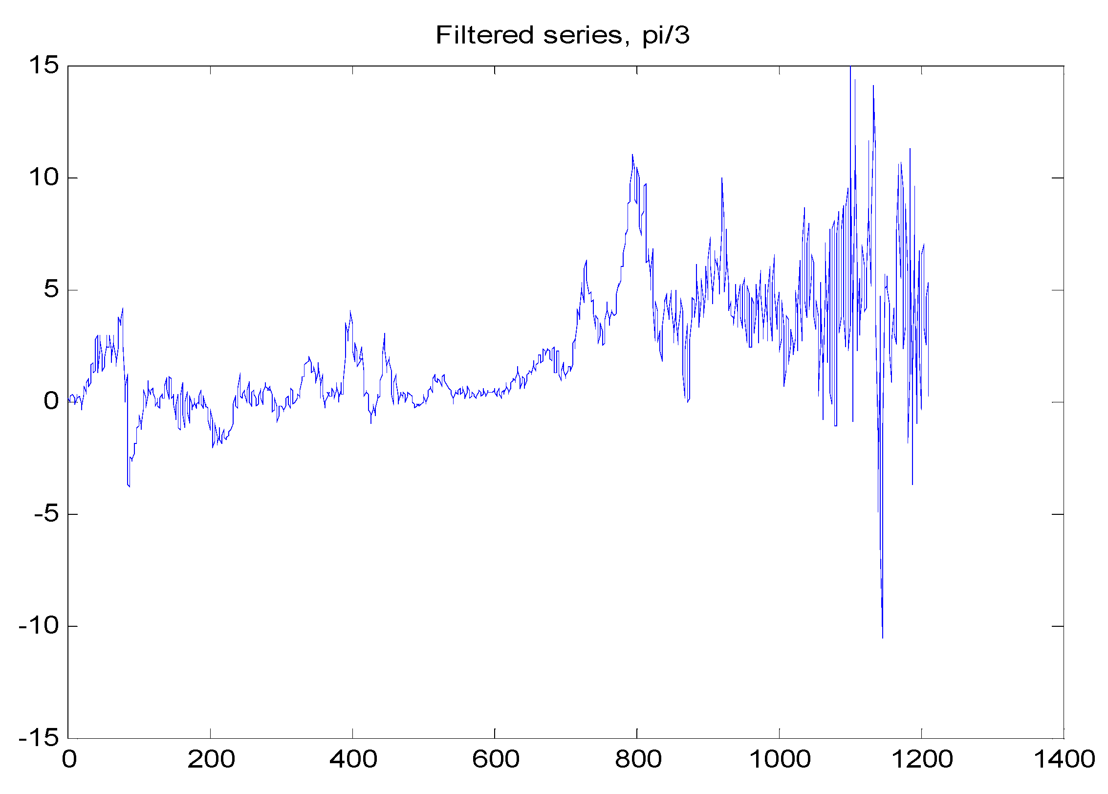
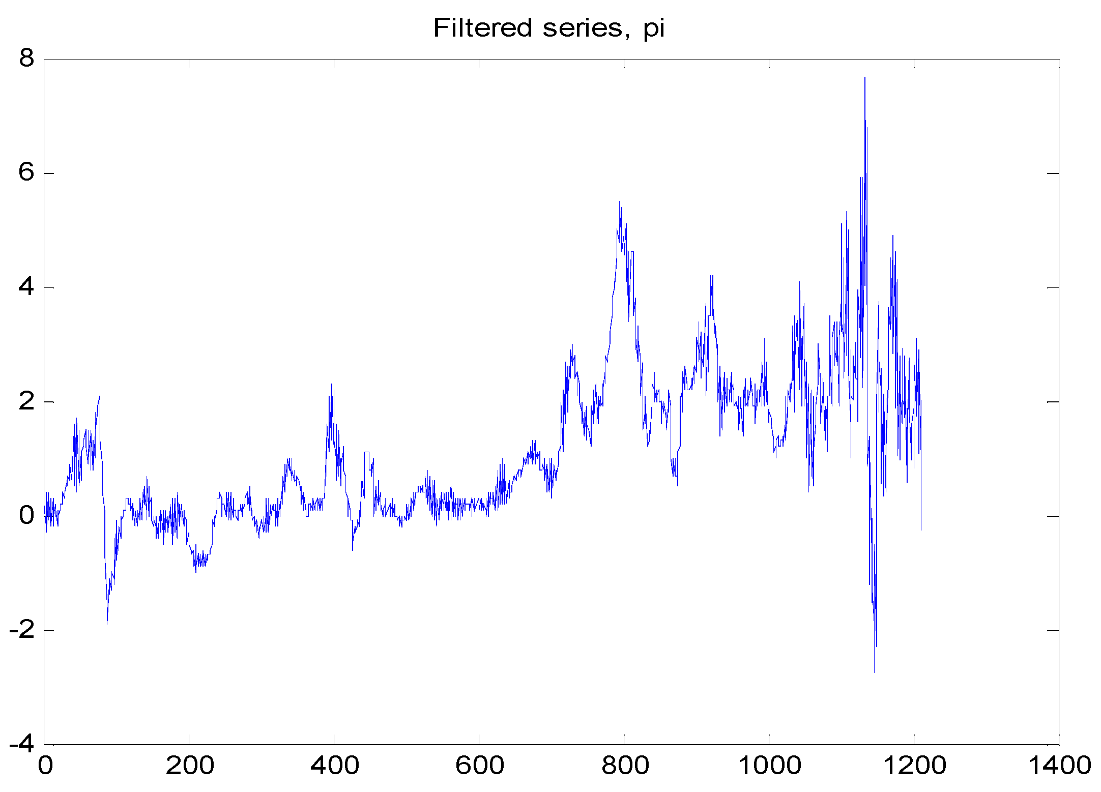
To test the seasonal stationarity against the presence of a seasonal unit root, it would be convenient to filter the series with a suitable filter that insulates the effects of other unit roots. For example, when testing the unit root at the Nyquist frequency, the series is filtered with
. However, when the aim is to test for the unit root at the harmonic frequency
, the used filter is
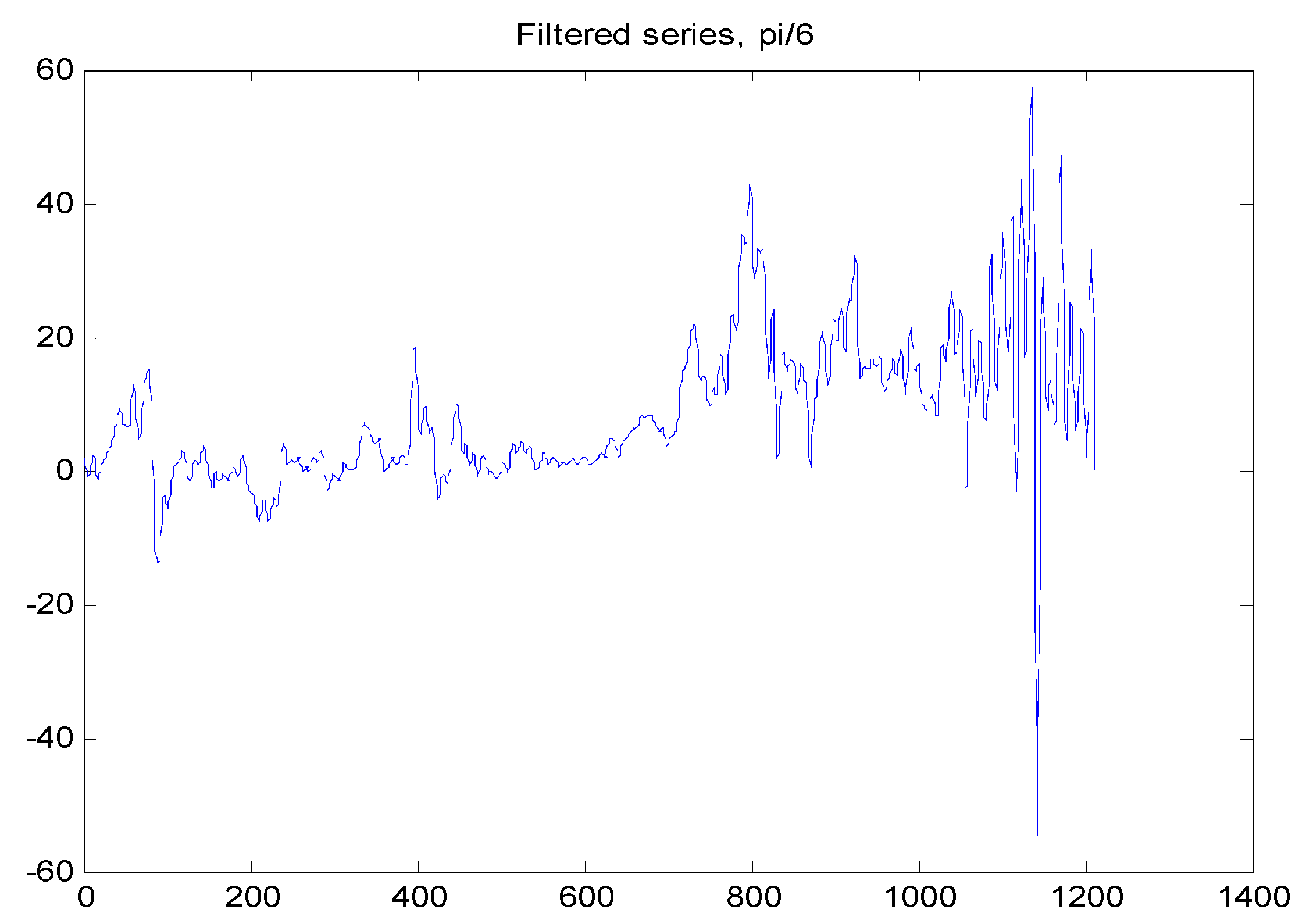
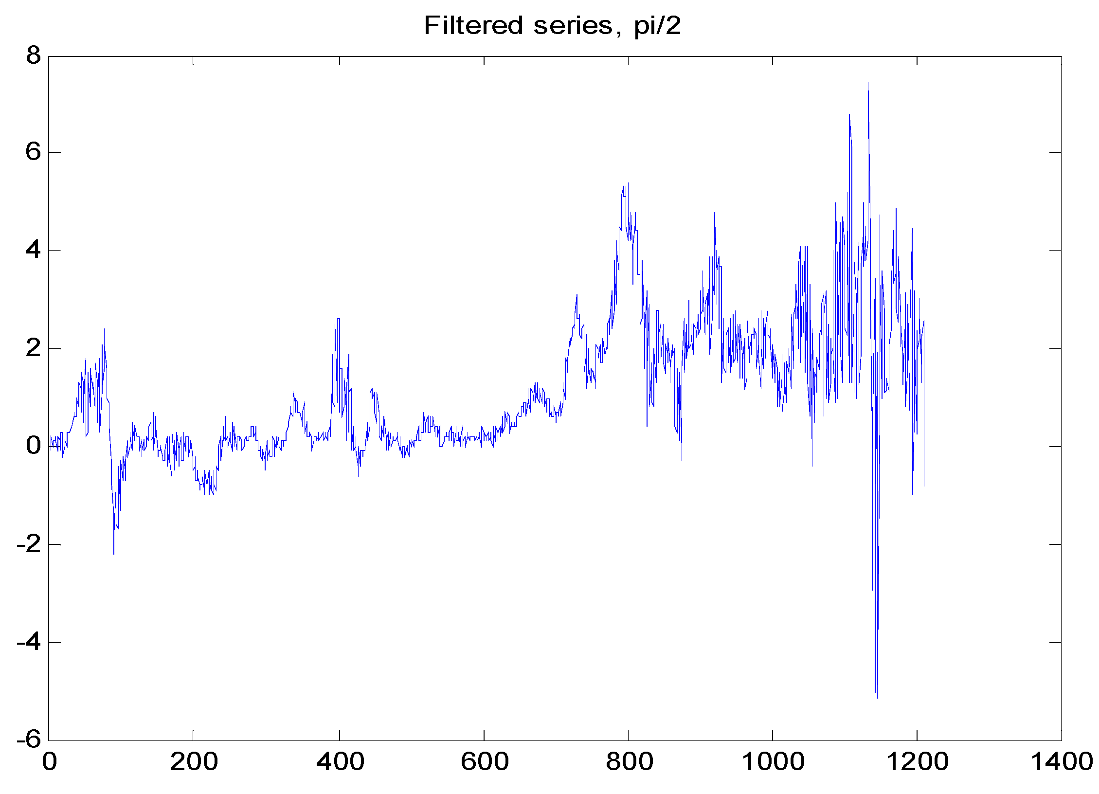
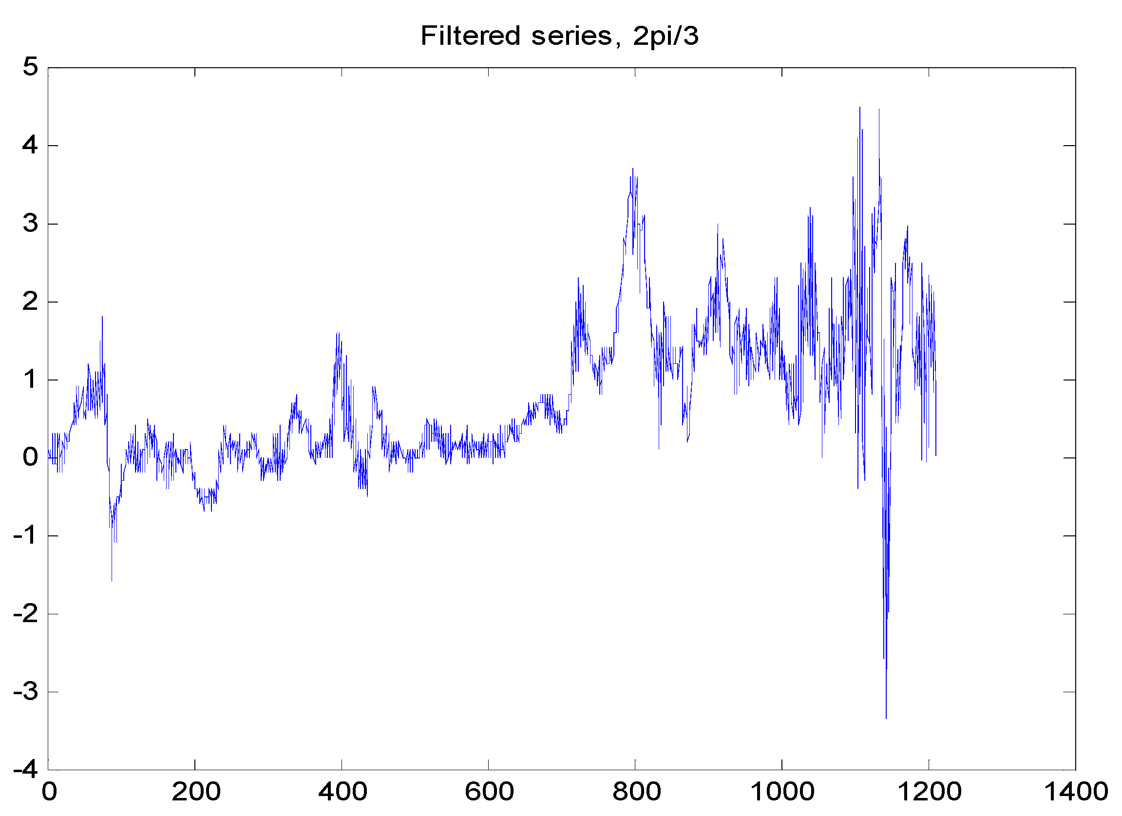
. All filters used to transform the data before testing contain the first difference filter so that all the obtained series are detrended and the trend movements in the CPI’s original series do not manifest themselves, as shown in
Figure 2,
Figure 3,
Figure 4,
Figure 5,
Figure 6 and
Figure 7. It is for this reason that the seasonal KPSS test is applied to these transformed series by considering only seasonal dummy variables,
i.e., trend deterministic components are not considered in the testing phase. For presentation purposes, the sample period is from January 1914 to December 2014 for all transformed series.
Figure 2.
The filtered series used in testing for the unit root at the frequency.
Figure 2.
The filtered series used in testing for the unit root at the frequency.
Figure 3.
The filtered series used in testing for the unit root at the frequency.
Figure 3.
The filtered series used in testing for the unit root at the frequency.
Figure 4.
The filtered series used in testing for the unit root at the frequency.
Figure 4.
The filtered series used in testing for the unit root at the frequency.
Figure 5.
The filtered series used in testing for the unit root at the frequency.
Figure 5.
The filtered series used in testing for the unit root at the frequency.
Figure 6.
The filtered series used in testing for the unit root at the frequency.
Figure 6.
The filtered series used in testing for the unit root at the frequency.
Figure 7.
The filtered series used in testing for the unit root at the Nyquist frequency.
Figure 7.
The filtered series used in testing for the unit root at the Nyquist frequency.
Before testing for seasonal stationarity, it would be informative to test for a conventional unit root. In this case, the series is filtered with the following filter: to isolate the effects of seasonal unit roots. Thus, the conventional KPSS test is used, concluding that a unit root is present in the CPI. The results are not reported here and can be obtained from the author upon request.
Table 5 summarizes the seasonal KPSS test results for testing unit roots corresponding to the seasonal frequencies associated with monthly data.
The main conclusion to be drawn from
Table 5 is that only the unit roots at frequencies
and
are not present, while there is good evidence that the other unit roots were accepted. In particular, the seasonal KPSS test concludes with the presence of the unit roots at the seasonal frequencies
,
and
, revealing that, respectively, one, two and three cycles were accomplished each year. The unit root at the Nyquist frequency is also present, indicating that six cycles were accomplished per year. Our results are quite similar to those of Coşar [
30], who found evidence of seasonal unit roots in the monthly series of the Turkish CPI.
Table 5.
The seasonal KPSS statistics corresponding to different units roots at seasonal frequencies in the monthly US CPI series.
Table 5.
The seasonal KPSS statistics corresponding to different units roots at seasonal frequencies in the monthly US CPI series.
| Statistics | | | |
|---|
| 2.6809 *** | 1.3040 *** | 1.5158 *** |
| 2.6796 *** | 2.9727 *** | 2.2646 *** |
| 1.2177 *** | 2.5996 *** | 1.6669 *** |
| 0.1259 | 0.2448 | 0.2013 |
| 0.0004 | 0.0047 | 0.0109 |
| 0.7023 ** | 1.6765 *** | 1.0650 *** |


