Real Option Valuation of an Emerging Renewable Technology Design in Wave Energy Conversion

Abstract

The untapped potential of wave energy offers another alternative to diversifying renewable energy sources and addressing climate change by reducing CO₂ emissions. However, development costs to mature the technology remain significant hurdles to adoption at scale and the technology often must compete against other marine energy renewables such as offshore wind. Here, we conduct a real option valuation that includes the uncertain market price of wholesale electricity and managerial flexibility expressed in determining future optimal decisions. We demonstrate the probability that the project’s embedded compound real option value can turn a negative net present value wave energy project to a positive expected value. This change in investment decision uses decision tree analysis, where real options are developed as decision nodes, and models the uncertainty as a risk-neutral stochastic process using chance nodes. We also show how our results are analogous to a financial out-of-the-money call option. Our results highlight the distribution of outcomes and the benefit of a staged long-term investment in wave energy systems to better understand and manage project risk, recognizing that these probabilistic results are subject to the ongoing evolution of wholesale electricity prices and the stochastic process models used here to capture their future dynamics. Lastly, we show that the near-term optimal decision is to continue to fund ongoing development of a reference architecture to a higher technology readiness level to maintain the long-term option to deploy such a renewable energy system through private investment or private–public partnerships.

1. Introduction

1.1. Motivation and Research Objectives

The world’s oceans and seas offer a variety of ways to generate renewable marine energy to help address climate change by diversifying power generation and reducing CO₂ emissions. In this article, we develop a valuation model of a nascent technology that harnesses the kinetic energy of waves to produce electricity. Termed wave energy conversion (WEC) technology, this form of marine energy has yet to be introduced at scale. Key contributors to this delay include levelized cost of energy (LCOE) estimates remaining higher than other marine energy alternatives, like offshore wind, and the lack of a standard design. However, Loth et al. (2022) suggest that the use of LCoE is questionable for renewables, like wind and solar, since this metric excludes the time-varying price of electricity. Further, Aldersey-Williams and Rubert (2019) illustrate that LCoE may also not include the volatile price of fuel and often provides a single value, rather than a distribution of outcomes. Lastly, to gain private financing, others have suggested that more traditional valuation measures should be used, like net present value (NPV).

“If very large wave energy installations are to be privately financed then this will involve pension funds and other very large investment funds and these investors will compare wave energy to other investment opportunities outside the power generation sector. In this case NPV or IRR should be preferred over LCoE.”.

—Pecher and Kofoed (2016, p. 116)

So, this paper will focus on developing an estimate of NPV to better inform non-governmental investors using a new and novel valuation approach to marine energy systems that uses real options. In the sections that follow, we will conduct a static investment analysis that determines NPV from a series of future cash flows and a discount rate. The cash flows will include revenues from WEC production and transmission to the wholesale electricity market. The electricity market is known to be volatile, so we model the uncertainty as a stochastic process to determine a distribution of cash flows, and subsequently a distribution of values. This financial valuation model also includes salient elements of a proposed WEC design and the cost impact of maturing it to technology readiness level (TRL) 9 when the designs may be implemented at scale. This study then applies the theory of real options, or options on real assets, to model the optimal decisions of future staged investments to obtain higher TRLs and undertake capital expenditures (CapExs).

1.2. Summary of Related Work and Our New Contribution

Economic models for energy project valuation are plentiful in the academic literature. The development of detailed cost models for a variety of different wave energy designs has been proposed by de Andrés et al. (2016, 2017), Tan et al. (2021), Biyela and Cronje (2016), Stansby et al. (2017), Guanche et al. (2014), and Lavidas and Blok (2021). Forecasting of energy prices and other commodities has also been carried out by a variety researchers, including Hahn et al. (2014), to forecast crude oil spot prices, and the seminal work by Black (1976), on forward contract pricing. And, real options analysis has been applied extensively to model energy markets and projects. Dalbem et al. (2014) applied real options to help support greater market efficiency, and Hahn and Dyer (2008) used real options to evaluate a switching option for an oil and natural gas project. However, to the best of our knowledge, this paper represents the first attempt at applying real options valuation models to the nascent technology of wave energy conversion.

2. Materials and Methods

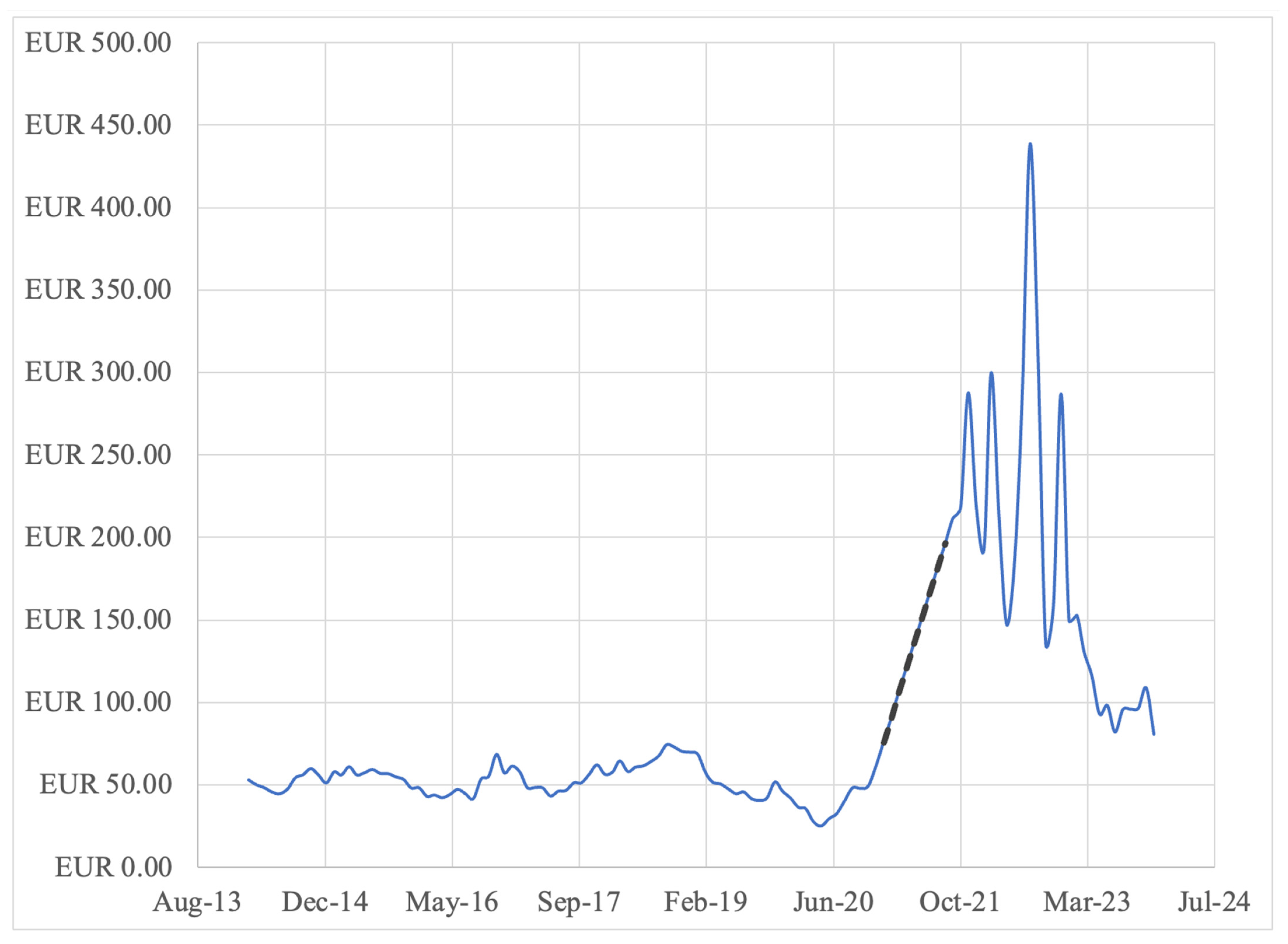
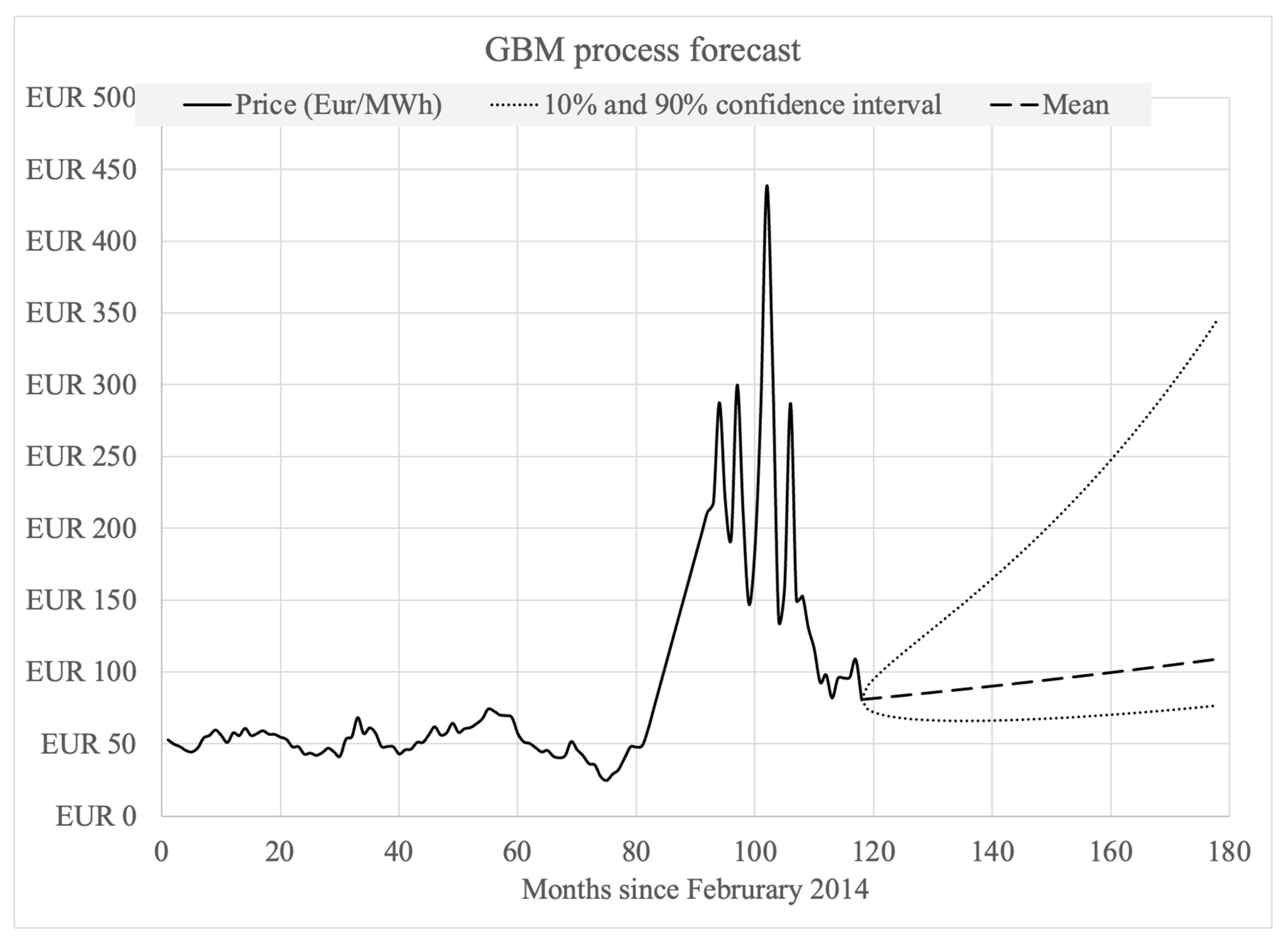
2.1. Energy Price Forecast with Uncertainty

We obtained data on wholesale market data for energy prices to support the cash flow and volatility inputs needed for real option valuation. We used data from the Nordpool Group (2024), which has a long history of promoting price transparency. We obtained monthly N2EX day-ahead auction prices from 108 months from March 2014 to December 2023. No data were available for the nine months of January–September, 2021, and the time series started in March 2014. A service specialist at the NordPool group indicated that Brexit was the cause for this interruption in data. However, our key conclusions were unaffected by this data interruption. Considering the break in these data in 2021, the 2014–2020 pricing data appear stationary, while the late 2021–2023 data are highly volatile and appear to be returning to a price of approximately EUR 100 per MWh. This time series appears in Figure 1. The higher prices and volatility in late 2021 to the end of 2023 could be caused by the combination of post-pandemic effects and other regional economic shocks disrupting regional energy markets in the region, as suggested by Lu et al. (2024).

To begin, we investigate the distribution of monthly returns, $r$, determined by the log of relative price, or

$$r=\ln (p_t/p_{t-1}),$$

(1)

where $p_t$ is the current month price and $p_{t-1}$ is the previous month’s price. The histogram of these returns appears in Figure 2. Visual inspection of Figure 2 suggests that the returns may be normal, but that the distribution could be leptokurtic due to what appears to be heavy tails. Indeed, the application of the Shapiro–Wilk test for normality produced a p-value less than 0.05. So, contrary to our visual inspection, this test indicates that the distribution is not normal. However, we also determined a kurtosis value of 4.7, which is an indicator of heavy tails, and a skewness of −0.8, which shows some degree of symmetry. So, we proceeded by removing six outliers from the sample that were in excess of ±40%. When we re-ran the Shapiro–Wilk test without these outliers, the Shapiro–Wilk test results were no longer statistically significant, suggesting that the heavy tails were the cause of the test results when outliers were included. We also performed the D’Agostino–Pearson test for normality, which yielded similar results and led us to the same conclusion that while the returns were not normally distributed, normality could be inferred by removing a few outliers. We believe our normality assumption is appropriate as the tests above with 95% of the sample observations included indicated this. Nevertheless, future work using alternative techniques, like the simulation of American options suggested by Longstaff and Schwartz (2001), could be applied to address this model limitation. Or, if the problem we model below could be re-cast as a European-style real option, models such as those suggested by Ziel and Steinert (2018) could be used.

The last statistical test we conducted was the augmented Dickey–Fuller test for mean reversion on the time series data appearing in Figure 1, which produced a p-value of 0.44. These results indicate that we could not conclude that the data were stationary over the decade worth of monthly data we analyzed. These results, suggesting long-term energy prices may follow a non-stationary process, are consistent with the findings of Hahn et al. (2014), who studied crude oil and drew from the commodity models originally proposed in the seminal work by Schwartz and Smith (2000). Consequently, we assumed that long-term prices can be reasonably modeled with a random walk, or more specifically as geometric Brownian motion (GBM), as suggested by Fama (1965) and used by Black and Scholes (1973).

To calibrate our GBM stochastic process to model price, we need to estimate growth and volatility terms for our stochastic differential equation as shown in Equation (2).

$$dP=\mu Pdt+\sigma Pdz,dz=ϵ\sqrt{dt},ϵ~N\left(\mathrm{0,1}\right)$$

(2)

Here, $dP$ is the change in price $P$, $\mu$ and $\sigma$ are the growth rate and volatility, and $dz$ represents the standard Wiener process. The last term in Equation (2) is the random variable from the standard normal distribution. This formulation is similar those found in Dalbem et al. (2014) and Dixit and Pindyck (1994).

We estimate the growth rate from a nonlinear curve fit of the equation

$$P_t=a_0{\mathrm{e}}^{rt}.$$

(3)

Taking the natural log of both sides and simplifying yields the linear equation

$$\ln \left(P_t\right)=\ln \left(a_0\right)+rt.$$

(4)

So, the slope of the natural log of the price will yield the estimated growth rate $r$. Then, the volatility$s$is estimated as the standard deviation of monthly returns. The growth rate is annualized by multiplying it by 12, and the volatility is annualized by multiplying it by $\sqrt{12}$, as supported by Benninga (2014). Consequently, using all the pricing data available yields annualized growth and volatility of 13.0% and 64.3%, respectively.

At this point, we did not believe that the future energy markets would support these values for a GBM forecast, given the economic shock that the wholesale electricity markets withstood in 2021–2023. We can see this by examining a monthly rolling volatility over 12-month periods. As shown in Figure 3, we see that prior to 2021, values were between 20% and 60%, and that current volatility appears to be returning to this range. So, for our forecasting of price and the real options analysis to follow, we assume a volatility of 40% as a baseline value.

Also, assuming wholesale electricity growth rates will likely return to lower values, we set our value for annualized price growth to 6%. Such a value is subjective, and could vary based on economic conditions like inflation, energy policies, technological advancements, and global energy markets. Nevertheless, it does capture wholesale nominal price increases and it is likely necessary to include these effects, similar to the assumptions made by Schwartz and Smith (2000) for processes with short-term and long-term components, or the jump processes described by Winston (2008). Using these values, our expected forecast with upper and confidence intervals at 10% and 90% levels appears in Figure 4. In the pro forma cash flow model in the next section, we will use the mean price forecast to determine our expected cash flows from operating a WEC system, similar to the approach used by Hahn et al. (2018).

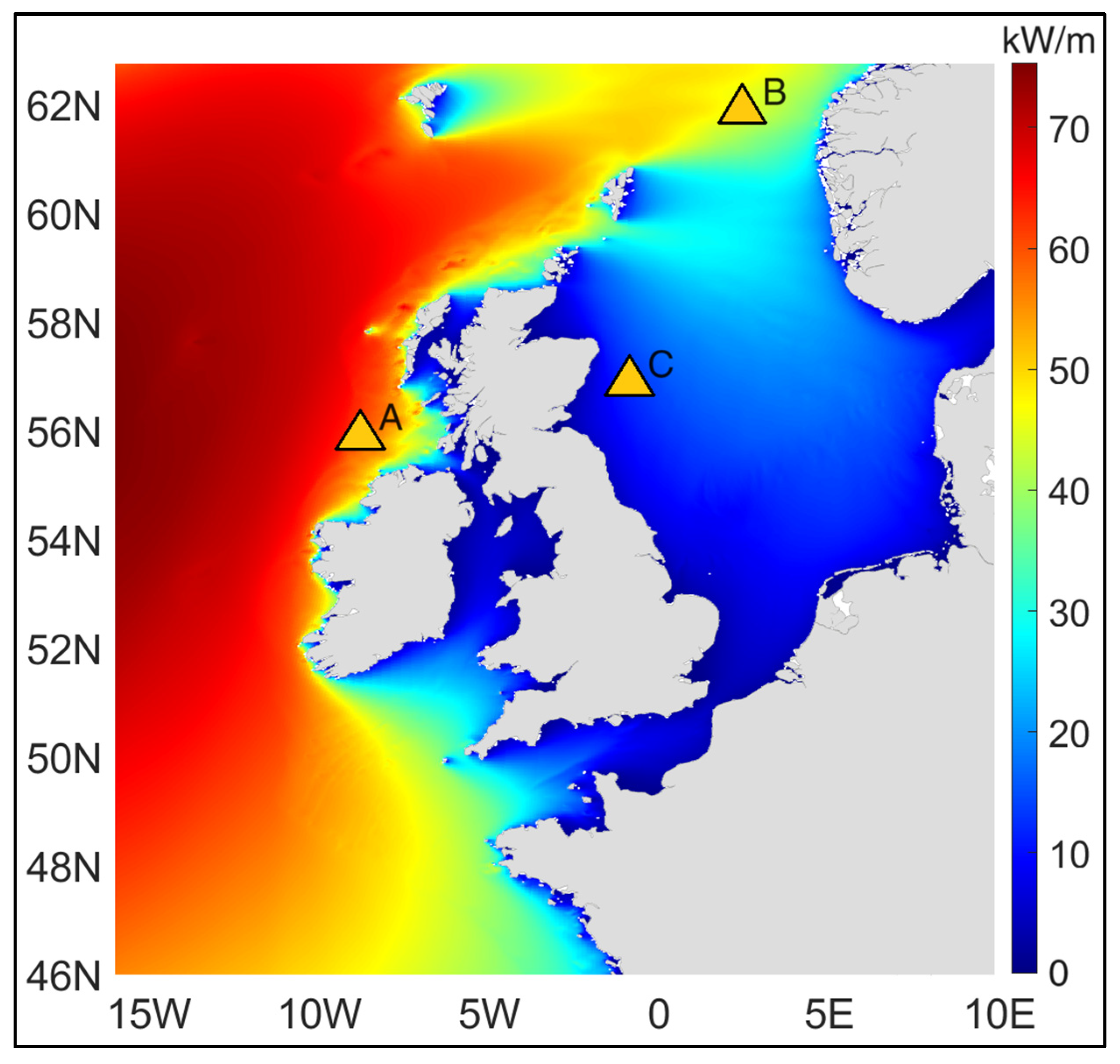
2.2. Site Selection and Annual Energy Production

Under the Market Asset Disclaimer suggested by Copeland and Antikarov (2003), we next developed a baseline model as our WEC system project without optionality. Carrying this out provides us with a complete market to support our real options analysis in the following section. We begin with modifying the Annual Energy Production (AEP) equation from Section 1.4.2 of Pecher and Kofoed (2016) to a Monthly Energy Production (MEP) estimate. The AEP can be found based on the following equation:

$$AEP={\sum }_{i=1}^{12}{MEP}_i,$$

(5)

where $ME{P}_i$ is the Monthly Energy Production for month i, where i = 1 for January, i = 2 for February, etc. So, we state that

$$MEP=P_{wave}\times widt{h}_{absorber}\times {\eta }_{w2w}\times availabilit{y}_{monthly}\times hour{s}_{monthly}\times n_{WEC}.$$

(6)

Here, $P_{wave}$ is wave power in kW/m and is location-dependent. This term represents the power per unit length available from ocean waves that can be converted to electricity. The next term, ${width}_{absorber}$, is the width of the WEC absorber in meters, and can vary based on the chosen WEC design. Generally speaking, a larger WEC will have a larger absorber, so can produce a larger amount of electricity. The third term, ${\eta }_{w2w}$, is the wave-to-wire efficiency as a percentage and is a weighted average over all wave conditions. It represents how well the technology is able to convert the wave power into electrical power, and can vary significantly depending on a system’s design. The next terms, ${availability}_{monthly}$ and ${hours}_{monthly}$, are the percent of time the WEC is producing each month and the total number of hours per month, respectively. Lastly, the term $n_{WEC}$ represents the number of WEC devices operating throughout the project’s lifecycle. This estimate is considered reasonably accurate at $\pm 50\%$ by Pecher and Kofoed (2016), which will be explored in the sensitivity analysis in the following section.

By using the variable ${hours}_{monthly}$, we include the effect of seasonality shown in O’Connell and Furlong (2021) and Rizaev et al. (2023). So, we can increase availability during peak months by deferring periodic maintenance until times of the year with lower wave power. We show below that the strongest wave power occurs in the winter months of December, January, and February and the weakest wave power occurs in the summer months of June, July, and August, so will assume higher availability in the winter months and lower availability during the summer months.

We next employ the long-term average of wave power from 42 years of Copernicus data1. The wave power $P_{wave}$ describes energy transmission by waves and encompasses both the significant wave height $H_s$ and the energy period $T_e$. Assuming irregular waves and deep water per unit crest length, $P_{wave}$ is given by

$$P_{wave}={\displaystyle \frac{\rho g^2}{64\pi }}{H}_s^2{T}_e\approx 0.49H_s^2{T}_e(\mathrm{k}\mathrm{W}/\mathrm{m})$$

(7)

where ρ is the sea water density (~1025 kg/m³), and g is the gravitational acceleration.

However, the sites we chose represent intermediate and deep waters, so an advanced calculation method was used. This method is formulated as a general wave energy assessment equation (GWEAE) and is defined by Liang et al. (2017).

$$P_{wave}={\displaystyle \frac{\pi \rho gD{H}_s^2}{16T_e}}\left[{\displaystyle \frac{1}{\mu }}+{\displaystyle \frac{2}{\sinh 2\mu }}\right]$$

(8)

Here, an explicit approximation of the linear dispersion relation µ is equal to Beji (2013). The details can also be found in Rizaev et al. (2023). The variable D is the water depth, which is estimated based on the numerical bathymetry model in Saulter (2021).

Table 1. Average Seasonal Wave Power for three sites considered in Figure 5, representing low, moderate, and high potential for a commercial wave energy system.

	Site	Winter (December, January, February)	Spring (March, April, May)	Summer (June, July, August)	Autumn (September, October, November)
$P_{wave}$ (kW/m)	A	109.634	48.3112	17.7887	55.9195
	B	84.3359	38.7219	12.5485	46.5122
	C	18.8204	10.389	4.5571	13.5729

shows the values for $P_{wave}$ at three locations around the United Kingdom that represent annual seasonal wave power from the 42 years of monthly Copernicus data. We assume these seasonal long-term averages will remain time-invariant for the purposes of our pro forma cash flow model.

Sites A, B, and C, along with the annual mean wave power, appear in Figure 5. The wave power estimation is based on an analysis forecast numerical wave model2 from the Copernicus Marine Environment Monitoring Service (CMEMS). The location considered for site A is a longitude of 8.5152° W and latitude of 55.9189° N, site B is a longitude of 2.4849° E and latitude of 62° N, and site C is a longitude of 1° W and latitude of 56.8919° N. From Figure 5, we see that similar to the seasonality of wave power shown in Table 1, site A has the highest wave power, followed by site B. Site C has the lowest wave power. These sites were chosen to represent best-, moderate-, and worst-case wave power locations to operate a WEC system in locations in relatively close proximity to the UK power grid.

The second, third, and fourth variables in our MEP model in Equation (6) are set according to

Table 2. Design parameters based on page 6 of Pecher and Kofoed (2016) and TALOS design from Sheng and Aggidis (2024).

Design Parameter	Value
$widt{h}_{absorber}$	30 m
${\eta }_{w2w}$	0.2
$availabilit{y}_{monthly}$	[December, January, February, March, April, May, June, July, August, September., October, November] = [0.99, 0.99, 0.99, 0.95, 0.95. 0.95, 0.9, 0.9, 0.9, 0.95, 0.95, 0.95]
$n_{WEC}$	25

.

2.3. Reference Design of a WEC from a TALOS Design

Note that the width of the absorber at 30 m is consistent with the TALOS WEC design as shown in Sheng and Aggidis (2023) and was used to measure wave conditions at the EMEC test site, Billia Croo, Scotland. The specific TALOS design used here is an optimized TALOS; the tailless TALOS, from Sheng and Aggidis (2024), appears below in Figure 6. The overall annual wave energy production, with the applications of an energy efficiency of 75% from the captured wave energy to electricity and a rated power of 625 kW, yields a corresponding capture factor of 0.243. While this production is about half the value for site B, and was chosen so that the test devices would not be subject to more severe wave conditions, the value for ${\eta }_{w2w}$ in Table 2 is a reasonable estimate which we expect to hold in a commercialized system under more severe wave conditions like those for sites A and B.

The availability design parameter in Table 2 includes seasonal adjustments to maximize winter season energy conversion and defer maintenance to the summer season. It also includes the need for the WEC system to enter survival mode during extreme weather events.

Using the values from Table 2, we determined 12 monthly MEP values and corresponding AEP values for sites A, B, and C. As previously noted, the values in

Table 3. Annual Energy Production from sites A, B, and C.

Site	AEP (MWh/Year)	AEP per WEC (MWh/Year)
A	73,005	2920
B	57,394	2296
C	14,869	595

are subject to an estimation error of $\pm$50%, as indicated by Pecher and Kofoed (2016).

2.4. Estimating Project Capacity

We assume the TALOS design is at TRL 6 in the following section to estimate likely costs. Following the Ocean Energy Systems (2015), AEP is defined as

$$AEP=capacity\times F\times availability\times 8760,$$

(9)

where 8760 is the number of hours per year, found by 24 h/day × 365 days/year. Here, capacity is the project capacity and F is the capacity factor, or alternatively called the load factor by a UK report from 2020 from the department of Department for Business, Energy & Industrial Strategy. From this UK report, $F\times availability$ = 30%. We can solve the system capacity as

$$Capacity=AEP/(F\times availability\times 8760)$$

(10)

Then, the capacities of the projects operating at sites A, B, and C from Table 3 are approximated as 27.8 MW, 21.8 MW, and 5.7 MW, respectively.

3. Cash Flow and Real Options Model

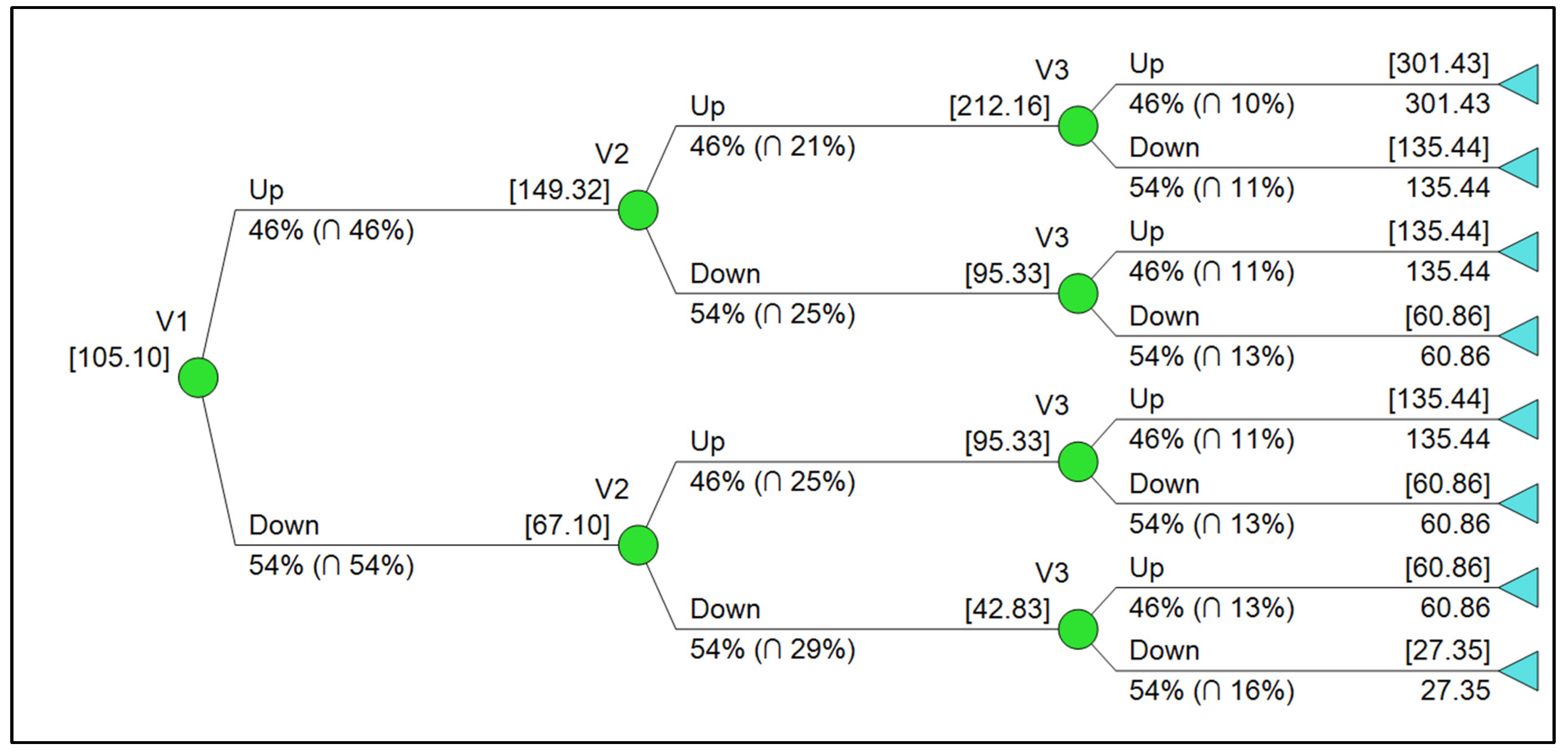
3.1. Underlying Model

We next infer the following cost parameters to complete our static financial model without optionality. We started with CapEx per AEP using Table 9 from Guo et al. (2023), which listed values between 0.041 and 0.455. We chose the largest of these values to avoid the use of the investment steps these authors used to reduce this expense, which is already inherent in the real option models to follow. The value for CapEx per AEP is also critical because we assume that annual OpEx is a fixed proportion shown in the second row of

Table 4. Baseline cost parameters and their sources.

Cost Parameter	Values	Source
CapEx per AEP (EUR/KWh)	EUR 0.455/KWh	Guo et al. (2023, p. 24)
OpEx/MWh, Year 1	5 to 15% of CapEx	Guo et al. (2023, p. 15)
TRL 6 to 7	EUR 10 to 15 M	Pecher and Kofoed (2016, p. 88)
TRL 7 to 8	EUR 10 to 15 M	Pecher and Kofoed (2016, p. 88)
TRL 8 to 9	EUR 20 to 100 M	Pecher and Kofoed (2016, p. 88)
Discount Rate	8 to 10%	Guo et al. (2023, p. 18).
Operating Years	20 to 50	Guo et al. (2023, p. 18).

, which is supported in the literature by de Andrés et al. (2016, 2017), Tan et al. (2021), Biyela and Cronje (2016), Stansby et al. (2017), Guanche et al. (2014), and Lavidas and Blok (2021).

For our other baseline cost estimates, we assume the midpoint values from Table 4. So, we set OpEx/MWh for Year 1 to 10%, TRL increases occur at the midpoint of their cost range, the discount rate is 9%, and the system operates for 35 years with no salvage value or decommissioning cost. We also ignore the implication of taxes, tariffs, and depreciation. For additional studies supporting this range of discount rates for wave energy conversion systems, please see Chang et al. (2018), Têtu and Fernandez Chozas (2021), Gray et al. (2017), and Chandrasekaran and Sricharan (2021). The convergence to a fairly narrow range of discount rates should help this study be more easily compared to previous ones. Also, firms wishing to further reduce the discount rate of a wave energy project could seek government-subsidized loans, which may be available at more favorable rates than the private debt markets can provide and materially alter the project’s capital structure.

3.2. Research, Development, CapEx, and OpEx Timelines

The timeline for the financial model includes sequential investments to improve TRL, followed immediately by CapEx, then by OpEx. The research and development phase for each TRL improvement lasts one year. So, we begin by assuming the TALOS design is at TRL 6. We invest today, Year 0, to move the technology from TRL 6 to 7. In Year 1, we invest again to move the technology from TRL 7 to 8. In Year 2, we invest to move the technology from TRL 8 to 9. Then, in Year 3, we invest for CapEx, to produce the WEC units and deploy them, at a present value of $P{V}_{CapEx}$. Lastly, in Year 4, we begin operation of the WEC system and selling electricity into the wholesale market, producing a present value in today’s dollars of ${PV}_{underlying}.$

So, the project’s NPV is expressed as

$$NPV=-P{V}_{TRL}-{\displaystyle \frac{P{V}_{CapEx}}{{\left(1+r_d\right)}^3}}+{\displaystyle \frac{P{V}_{underlying}}{{\left(1+r_d\right)}^4}},$$

(11)

where $r_d$ is the project’s discount rate, and

$$P{V}_{TRL}=P{V}_{6-7}+{\displaystyle \frac{P{V}_{7-8}}{\left(1+r_d\right)}}+{\displaystyle \frac{P{V}_{8-9}}{{\left(1+r_d\right)}^2}}.$$

(12)

Using the midpoint values for TRL increases and the discount rate shown in Table 4, we find that $P{V}_{TRL}=$ € 74.5 M. We then determine the CapEx and the annual OpEx for sites A, B, and C, with results appearing in

Table 5. Costs, operational value, and NPV estimates for sites A, B, and C. All values in Euros (EUR).

Site	${\mathit{P}\mathit{V}}_{\mathit{T}\mathit{R}\mathit{L}}$	${\mathit{P}\mathit{V}}_{\mathit{C}\mathit{a}\mathit{p}\mathit{E}\mathit{x}}$	${\mathit{P}\mathit{V}}_{\mathit{u}\mathit{n}\mathit{d}\mathit{e}\mathit{r}\mathit{l}\mathit{y}\mathit{i}\mathit{n}\mathit{g}}$	NPV
A	74.5 M	33.2 M	105.1 M	−25.7 M
B	74.5 M	26.1 M	82.6 M	−36.1 M
C	74.5 M	6.77 M	21.4 M	−64.5 M

. To include increasing future operational costs, we set an OpEx annual growth rate of 4%. To determine the net cash flow for each year, we assume first year operations generate revenue at a rate of EUR 100/MWh, which grows at a rate of 6% per year. Subtracting the annual OpEx from these revenues and discounting the cash flows at 9% yields a $P{V}_{underlying}$ as shown in the fourth column in Table 5. Combining Equations (11) and (12) then produces the NPV in the last column of Table 5. Note that the underlying present value is a critical input to our real options analysis to follow, as it is analogous to the stock price in financial call options.

As the results in Table 5 show, negative NPVs occur for all the sites. So, we can characterize these as out-of-the-money call options. But, prior to investigating the option value in this project, we perform a sensitivity analysis in the next section to see which factors in this deterministic model have the greatest impact on NPV.

To validate our cost assumption, we note that the combination of TRL and CapEx costs in Table 5 sum to approximately EUR 100 M for sites A and B. For a system capacity of approximately 25 MW, estimated in the previous section, and using the total CapEx Factor of EUR 4 M/MW from Table 7 of Ocean Energy in the European Union (2022) for systems with capacity greater than 20 MW, we confirm that this EUR 100 M total investment is an appropriate cost estimate at this stage in the TALOS design. Nevertheless, given the uncertainty of these cost estimates, the following section conducts a detailed sensitivity analysis.

3.3. Sensitivity Analysis

To conduct a sensitivity analysis, we evaluated site A and varied each of the following variables individually. The baseline values used previously, along with high and low values, appear below in

Table 6. Low, baseline, and high values for sensitivity analysis. All values in Euros (EUR).

Variable	Low	Baseline	High
P_wave factor	0.5	1.0	1.5
Expected growth rate of wholesale electricity prices	3%	6%	7.5%
Discount rate	8%	9%	10%
CapEx per AEP (EUR/KWh)	0.2275	0.455	0.6825
OpEx/MWh for Year 1	22.75	45.5	68.25
OpEx growth rate	2%	4%	6%
TRL 6 to 7 (M EUR)	10	12.5	15
TRL 7 to 8 (M EUR)	10	12.5	15
TRL 8 to 9 (M EUR)	20	60	100

.

We then estimated the NPVs for each of these combinations and sorted them from the largest absolute change to the smallest. So, the top row of Table 6 shows which variable has the largest impact on NPV, and the last rows show the variable with the smallest impact on NPV.

Table 7. NPV sensitivity to model variables, sorted from largest to smallest absolute change, site A.

Variable	NPV Low	NPV Baseline	NPV High
TRL 8 to 9 (M EUR)	9	−25.7	−59.3
Expected growth rate of wholesale electricity prices	−63	−25.7	2.8
CapEx per AEP (EUR/KWh)	6.9	−25.7	−58.2
P_wave factor	−50	−25.7	−1.3
OpEx/MWh for Year 1	−5.9	−25.7	−45.4
Discount rate	−12	−25.7	−36.2
OpEx growth rate	−17	−25.7	−38
TRL 6 to 7 (M EUR)	−23	−25.7	−28.2
TRL 7 to 8 (M EUR)	−23	−25.7	−28

shows that a WEC project’s valuation is most sensitive to TRL 8 to 9, the growth rate of wholesale electricity prices, and CapEx. However, the project’s NPV is least sensitive to TRL increases from 6 to 7 and 7 to 8. This latter result supports our findings in the next section indicating that the relatively low cost of this research and development phase has little effect on the overall project’s profitability. We expect to see a similar trend for sites B and C, so we do not include them here. Instead, we focus the next sections on the option value that may be part of a project like this one. We also note that, in nearly all cases, the high NPVs usually remain negative. So, in the next section, we explore if (or when) there is enough option value to change the baseline NPV from negative to positive by modeling the problem like an out-of-the-money call option.

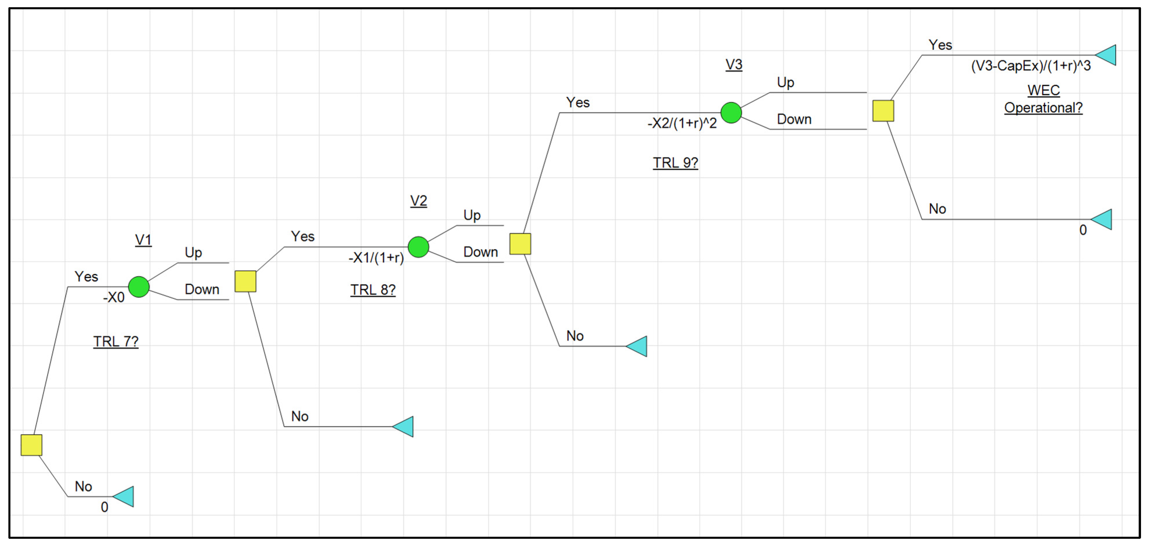
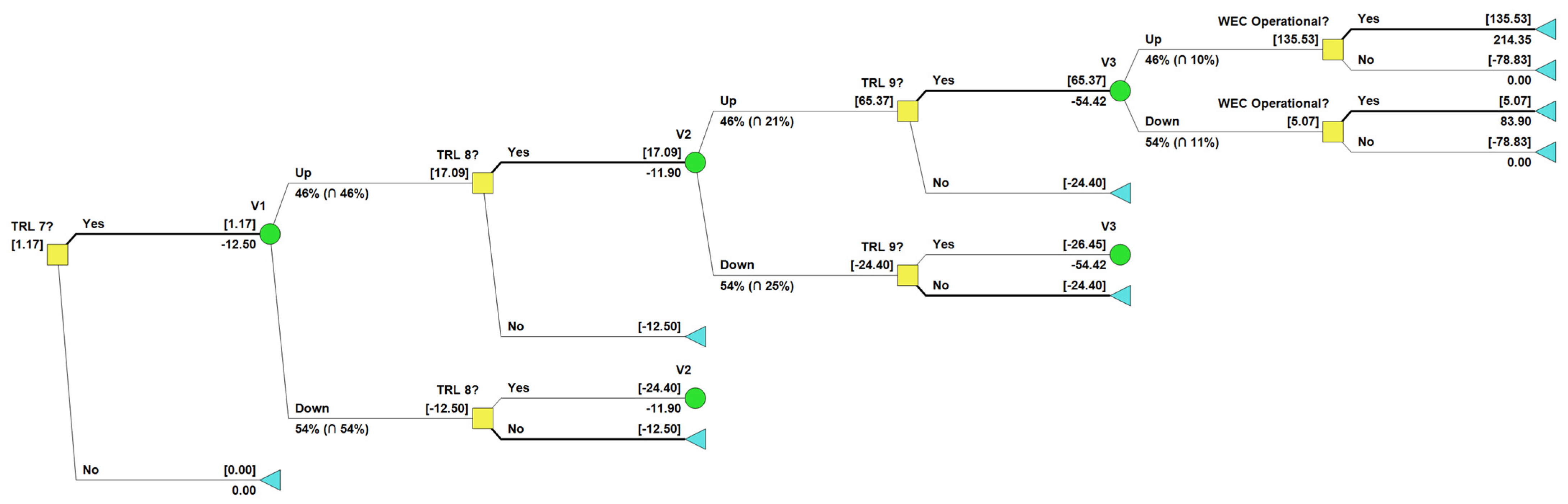
3.4. Risk-Neutral Valuation of the Option to Increase TRL and Operate the WEC System

We next implement a decision tree approach with a binomial lattice to model the underlying uncertain cash flows using a risk-neutral valuation methodology. By using a risk-neutral approach, we may determine the option value by discounting future cash flows at the risk-free rate. Thus, the option value determined below is independent of the project’s discount rate. This risk-neutral valuation of a compound option is similar to the compound option found in Copeland and Tufano (2004) and DiLellio (2022), where prior investments were required before production and associated cash flows could occur to yield ${PV}_{underlying}$. The figure below shows the structure of the decision tree associated with this compound option using the commercial decision analysis package DPL^® from Syncopation software, version 9.

In Figure 7, the project starts today with an investment of X0 to reach TRL 7. If this investment is not made, then the project is over and the NPV is 0. However, if the TRL 7 investment is made, then TRL 7 is achieved in one year. The next decision is whether to invest EUR X1 to reach TRL 8. If this next investment is made, another year passes. Otherwise, the project ends with an NPV of −X0. The final investment to reach TRL 9 must be decided upon at a cost of EUR X2. If TRL 9 is not pursued, then the project’s NPV is −X0 − X1/(1 + r), where r is the risk-free rate.

If the TRL 9 investment is made, another year passes, and now we have the option to invest CapEx to build the system, which produces uncertain cash flows, V3, based on the value of the underlying shown in Table 5. Figure 8 shows how a non-recombining binomial lattice, based on Cox et al. (1979), models the uncertainty in ${PV}_{underlying}$, assuming a risk-free rate $r$ equal to 5%. The underlying lattice values were found based on up and down factors (u and d) and associated risk-neutral probabilities (p), which are shown by Cox et al. (1979) with $\mathsf{\Delta }t$ = 1 year and $\sigma =40\%$.

$$u=e^{\sigma },d={\displaystyle \frac{1}{u}},p={\displaystyle \frac{1+r+d}{u-d}}$$

(13)

While Figure 8 is for site A, similar models for the underlying project’s uncertain values were produced for sites B and C, but are not included for the sake of space. Also, note that Cox et al. (1979) generate a recombining lattice, where n periods produce n + 1 unique terminal values. In this example, the three-period model has four unique terminal nodes. However, using a decision tree provides greater flexibility and does not assume that terminal nodes re-combine at the small additional cost of computational time. So, for this three-period model, there are eight terminal nodes. Nevertheless, the computational results are unaffected. Lastly, the up and down values shown here correspond to a risk-neutral valuation approach, so that future values may be discounted at the risk-free rate. Also, risk-neutral valuation does not require additional future uncertainty states after the decision to make the WEC operational since there are no later downstream decisions in the decision tree in Figure 7.

As Figure 8 shows, the uncertainty of the future wholesale electricity prices at a 40% volatility could yield a present value of the underlying project as high as EUR 323 M, or as low as EUR 29.3 M once operations begin. Then, terminal nodes also show the conditional probabilities to reach the outcome, which provides a discrete approximation of a log-normal distribution.

4. Results and Discussion

Baseline Model Valuation with Option to Deploy

Applying this underlying uncertainty to our decision tree in Figure 7 produces a positive NPV for sites A and B, but not for site C. These values are summarized in

Table 8. Expected NPV for WEC system with optionality.

Site	Expected NPV
A	EUR 12.6 M
B	EUR 1.17 M
C	EUR 0.0 M

.

Details of the decision tree for site A appear in Figure 9 and those for site B appear in Figure 10. We exclude the policy tree for site C, as it has no value. That means that there is no option value for site C and there are no conditions where site C should be pursued for investment. Put another way, if site C were the only site available for investment, neither investing to achieve higher TRLs nor CapEx investments should be made.

However, sites A and B do have significant option value. They also offer insights into how these optimal decisions were obtained. In both cases, it was always optimal to invest in reaching TRL 7. However, if wholesale electricity prices and their corresponding expectations on future cash flows are low, then it is never optimal to pursue TRL 8. After the TRL 8 investment decision, optimal decisions change for site A and site B.

For site A, it is always optimal to invest in TRL 9, then build and operate the WEC system at site A for the next 35 years. There is a 46% chance of making the investment reach TRL 8, as shown in the “Up” branch after the decision to invest in TRL 7 is made. Ultimately, the WEC system has positive NPVs in three out of the four uncertain project values. As shown in the upper right portion of Figure 9, there is a 10% chance of an NPV of EUR 193.9 M, and a 22% chance of an NPV of EUR 27.9 M. And, there is a 13% chance of an EUR −46.7 M NPV. While this last outcome is not preferred, it is statistically better than simply avoiding CapEx and OpEx, and not deploying a WEC system to produce electricity for wholesale markets.

However, at site B, conditions are less favorable. If the value of the underlying goes down in the second year after going up in the first year, then the project is no longer worth pursuing, so investments in TRL 9, CapEx, and OpEx will not be made. However, if conditions are favorable at site B after both the 1st and 2nd year, then the investments in TRL 9, CapEx, and OpEx should be made, thereby producing a series of cash flows for the next 35 years.

5. Conclusions

This analysis demonstrates that an investment in increasing the TRL of a WEC system and fielding and operating it is similar to a financial out-of-the-money compound call option whose value depends on future electricity prices. Based on a site survey of wave energy expectations, we show that all three sites produce negative NPVs without optionality, indicating they are not worthy of investment. Our sensitivity analysis largely supports this conclusion. However, when the investment problem is considered as a compound option, we see that two of the three sites can produce a positive expected NPV when future wholesale electricity prices are higher than expected. Our results show a distribution of outcomes and the benefits of a staged long-term investment in wave energy systems to better understand and manage project risk. We also recognize that these probabilistic results are subject to the ongoing evolution of wholesale electricity prices and the stochastic process models used here to capture their future dynamics. Lastly, we show that the near-term optimal decision is to continue to fund ongoing development of a reference architecture to a higher technology readiness level to maintain the long-term option to deploy such a renewable energy system through private investment or public–private partnerships. This simple but demonstrative analysis shows how often such payoffs may occur as a proxy for investor risk. This work also shows that investors should consider probabilistic estimates of value from an optimal decision framework enabled by real options analysis when considering investments that are not yet at TRL 9.

Future work in this area could explore the long-term secular trends in wave energy, as recently examined by Chen (2024) and Liu et al. (2024), as these types of energy systems will likely operate for many decades. Similarly, as the TRL increases, the wave power estimation error can be decreased by using a power matrix suggested by Babarit et al. (2012) and Guillou et al. (2020). One can also determine the levelized avoided cost of energy (LACE) and the levelized cost of energy (LCOE) by applying a framework proposed by Beiter et al. (2017) to align with metrics utilized by government agencies interested in public–private partnerships with private capital investors. Lastly, researching the benefits of additional real options to represent scalability and other managerial flexibilities will help investors and policy makers see the option value inherent in these nascent systems. As the world continues to seek out renewable energy sources to reduce CO₂ emissions, rigorous valuations and economic analyses are critical to help guide decision makers support future clean energy goals.

References

1. Aldersey-Williams, J., & Rubert, T. (2019). Levelised cost of energy—A theoretical justification and critical assessment. Energy Policy, 124, 169–179. [Google Scholar] [CrossRef]
2. Babarit, A., Hals, J., Muliawan, M., Kurniawan, A., Moan, T., & Krokstad, J. (2012). Numerical benchmarking study of a selection of wave energy converters. Renewable Energy, 41, 44–63. [Google Scholar] [CrossRef]
3. Beiter, P., Musial, W., Kilcher, L., Maness, M., & Smith, A. (2017). An assessment of the economic potential of offshore wind in the United States from 2015 to 2030 (National Renewable Energy Laboratory Technical Report NREL/TP-6A20-67675). National Renewable Energy Laboratory (NREL). [Google Scholar]
4. Beji, S. (2013). Improved explicit approximation of linear dispersion relationship for gravity waves. Coastal Engineering, 73, 11–12. [Google Scholar] [CrossRef]
5. Benninga, S. (2014). Financial modeling (4th ed.). MIT Press. [Google Scholar]
6. Biyela, S., & Cronje, W. (2016). Techno-economic analysis framework for wave energy conversion schemes under South African conditions: Modeling and simulations. International Journal of Energy and Power Engineering, 10, 786–792. [Google Scholar]
7. Black, F. (1976). The pricing of commodity contracts. Journal of Financial Economics, 3, 167–179. [Google Scholar] [CrossRef]
8. Black, F., & Scholes, M. (1973). The pricing of options and corporate liabilities. Journal of Political Economy, 81(3), 637–654. [Google Scholar] [CrossRef]
9. Chandrasekaran, S., & Sricharan, V. V. S. (2021). Numerical study of bean-float wave energy converter with float number parametrization using WEC-Sim in regular waves with the Levelized Cost of Electricity assessment for Indian sea states. Ocean Engineering, 237, 109591. [Google Scholar] [CrossRef]
10. Chang, G., Jones, C. A., Roberts, J. D., & Neary, V. S. (2018). A comprehensive evaluation of factors affecting the levelized cost of wave energy conversion projects. Renewable Energy, 127, 344–354. [Google Scholar] [CrossRef]
11. Chen, W. B. (2024). Analysing seven decades of global wave power trends: The impact of prolonged ocean warming. Applied Energy, 356, 122440. [Google Scholar] [CrossRef]
12. Copeland, T. E., & Antikarov, V. (2003). Real options, revised edition: A practitioners guide. Texere. [Google Scholar]
13. Copeland, T. E., & Tufano, P. (2004). A real-world way to manage real options. Harvard Business Review. [Google Scholar]
14. Cox, J., Ross, S., & Rubinstein, M. (1979). Option pricing: A simplified approach. Journal of Financial Economics, 7(3), 229–263. [Google Scholar] [CrossRef]
15. Dalbem, M., Brandao, L., & Gomes, L. (2014). Can the regulated market help foster a free market for wind energy in Brazil? Energy Policy, 66, 303–311. [Google Scholar] [CrossRef]
16. de Andrés, A., Maillet, J., Todalshaug, J., Möller, P., Bould, D., & Jeffrey, H. (2016). Techno-economic related metrics for a wave energy converters feasibility assessment. Sustainability, 8, 1109. [Google Scholar] [CrossRef]
17. de Andrés, A., Medina-Lopez, E., Crooks, D., Roberts, O., & Jeffrey, H. (2017). On the reversed LCOE calculation: Design constraints for wave energy commercialization. International Journal of Marine Energy, 18, 88–108. [Google Scholar] [CrossRef]
18. DiLellio, J. (2022). Real option modeling and valuation: A decision analysis approach using DPL and Excel (3rd ed.). Amazon. [Google Scholar]
19. Dixit, K., & Pindyck, R. (1994). Investment under uncertainty. Princeton University Press. [Google Scholar]
20. Fama, E. (1965). The behavior of stock-market prices. Journal of Business, 64, 34–105. [Google Scholar] [CrossRef]
21. Gray, A., Dickens, B., Bruce, T., Ashton, I., & Johanning, L. (2017). Reliability and O&M sensitivity analysis as a consequence of site specific characteristics for wave energy converters. Ocean Engineering, 141, 493–511. [Google Scholar]
22. Guanche, R., de Andrés, A., Simal, P., Vidal, C., & Losada, I. (2014). Uncertainty analysis of wave energy farms financial indicators. Renewable Energy, 68, 570–580. [Google Scholar] [CrossRef]
23. Guillou, N., Lavidas, G., & Chapalain, G. (2020). Wave energy resource assessment for exploitation—A review. Journal of Marine Science and Engineering, 8, 705. [Google Scholar] [CrossRef]
24. Guo, C., Shen, W., De Silva, D., & Aggidis, G. (2023). A review of the levelized cost of wave energy based on a techno-economic model. Energies, 16(5), 2144. [Google Scholar] [CrossRef]
25. Hahn, W., DiLellio, J., & Dyer, J. (2014). What do market-calibrated stochastic processes indicate about the long-term price of crude oil? Energy Economics, 44, 212–221. [Google Scholar] [CrossRef]
26. Hahn, W., DiLellio, J., & Dyer, J. (2018). Risk premia in commodity price forecasts and their impact on valuation. Energy Economics, 72, 393–403. [Google Scholar] [CrossRef]
27. Hahn, W., & Dyer, J. (2008). Discrete time modeling of mean-reverting stochastic processes for real option valuation. European Journal of Operational Research, 184, 534–548. [Google Scholar] [CrossRef]
28. Lavidas, G., & Blok, K. (2021). Shifting wave energy perceptions: The case for wave energy converter (WEC) feasibility at milder resources. Renewable Energy, 170, 1143–1155. [Google Scholar] [CrossRef]
29. Liang, B., Shao, Z., Wu, G., Shao, M., & Sun, J. (2017). New equations of wave energy assessment accounting for the water depth. Applied Energy, 188, 130–139. [Google Scholar] [CrossRef]
30. Liu, J., Li, R., Li, S., Meucci, A., & Young, I. R. (2024). Increasing wave power due to global climate change and intensification of Antarctic Oscillation. Applied Energy, 358, 122572. [Google Scholar] [CrossRef]
31. Longstaff, F. A., & Schwartz, E. S. (2001). Valuing American options by simulation: A simple least-squares approach. Review of Financial Studies, 14(1), 113–147. [Google Scholar] [CrossRef]
32. Loth, E., Qin, C., Simpson, J. G., & Dykes, K. (2022). Why we must move beyond LCOE for renewable energy design. Advances in Applied Energy, 8, 100112. [Google Scholar] [CrossRef]
33. Lu, S., Coutts, K., & Gudgin, G. (2024). Energy shocks and inflation episodes in the UK. Energy Economics, 129, 107208. [Google Scholar] [CrossRef]
34. Nordpool Group. (2024). Day ahead auction average prices. Nordpool Group. [Google Scholar]
35. Ocean Energy in the European Union. (2022). Status report on technology development, trends, value chains and markets. European Commission Joint Research Centre. [Google Scholar]
36. Ocean Energy Systems. (2015). International levelised cost of energy for ocean energy technology. IEA Technology Collaboration Programme for Ocean Energy Systems (OES). [Google Scholar]
37. O’Connell, R., & Furlong, R. (2021, September 16–17). An assessment of newly available Copernicus sea surface wave products for mapping wave energy in Irish and UK waters. Proceedings of the 14th CoastGIS International Symposium, Raseborg, Finland. [Google Scholar]
38. Pecher, A., & Kofoed, J. P. (2016). Handbook of ocean wave energy. Springer. [Google Scholar]
39. Rizaev, I. G., Dorrell, R. M., Oikonomou, C. L., Tapoglou, E., Hall, C., Aggidis, G. A., & Parsons, D. R. (2023). Wave power resource dynamics for the period 1980–2021 in Atlantic Europe’s Northwest Seas. In ISOPE international ocean and polar engineering conference (p. ISOPE-I). ISOPE. [Google Scholar]
40. Saulter, A. (2021). North West European shelf Production Centre NWSHELF_REANALYSIS_WAV_004_015 (Issue 1.1). Copernicus Marine Environment Monitoring Service Quality Information Document. Copernicus Marine Service. [Google Scholar]
41. Schwartz, E., & Smith, J. (2000). Short-term variations and long-term dynamics in commodity prices. Management Science, 46(7), 893–911. [Google Scholar] [CrossRef]
42. Sheng, W., & Aggidis, G. (2023, June 18–23). Hydrodynamic comparisons of TALOS wave energy converter using panel methods. Proceedings of the 33rd International Ocean and Polar Engineering Conference, ISOPE-2023, Ottawa, ON, Canada. [Google Scholar]
43. Sheng, W., & Aggidis, G. (2024, June 16–21). Optimizations for improving energy absorption of TALOS WEC. Proceedings of the 34th International Ocean and Polar Engineering Conference, ISOPE-2024, Rhodes, Greece. [Google Scholar]
44. Stansby, P., Moreno, E., & Stallard, T. (2017). Large capacity multi-float configurations for the wave energy converter M4 using a time-domain linear diffraction model. Applied Ocean Research, 68, 53–64. [Google Scholar] [CrossRef]
45. Tan, J., Polinder, H., Laguna, A., Wellens, P., & Miedema, S. (2021). The influence of sizing of wave energy converters on the techno-economic performance. Journal of Marine Science and Engineering, 9, 52. [Google Scholar] [CrossRef]
46. Têtu, A., & Fernandez Chozas, J. (2021). A proposed guidance for the economic assessment of wave energy converters at early development stages. Energies, 14, 4699. [Google Scholar] [CrossRef]
47. Winston, W. (2008). Financial models using simulation and optimization II: Investment valuation, options pricing, real options, & product pricing models. Palisade Corporation. [Google Scholar]
48. Ziel, F., & Steinert, R. (2018). Probabilistic mid- and long-term electricity price forecasting. Renewable and Sustainable Energy Reviews, 94, 251–266. [Google Scholar] [CrossRef]
Figure 1. Time series of UK wholesale electricity prices.
Econometrics 13 00011 g001
Figure 2. Histogram of monthly returns of UK wholesale electricity prices, 2014–2023.
Econometrics 13 00011 g002
Figure 3. Twelve-month rolling annualized volatility, 2014–2023.
Econometrics 13 00011 g003
Figure 4. GBM process forecast for wholesale electricity prices.
Econometrics 13 00011 g004
Figure 5. Climatological annual mean wave power, 1980–2021.
Econometrics 13 00011 g005
Figure 6. The tailless TALOS (displacement: 2969 m3).
Econometrics 13 00011 g006
Figure 7. Decision tree for compound option.
Econometrics 13 00011 g007
Figure 8. Non-recombining lattice to model the uncertain value of the underlying project’s cash flows for site A.
Econometrics 13 00011 g008
Figure 9. Policy tree for site A with an expected NPV of EUR 12.6 M.
Econometrics 13 00011 g009
Figure 10. Policy tree for site B with an expected NPV of EUR 1.17 M.
Econometrics 13 00011 g010