
Parameter Estimation of the Heston Volatility Model with Jumps in the Asset Prices


Abstract
1. Introduction
2. Heston Model without and with Jumps
2.1. Model Characterisation
2.2. Euler–Maruyama Discretisation
3. Estimation Framework
3.1. Regular Heston Model
3.1.1. Estimation of
3.1.2. Estimation of , , and
3.1.3. Estimation of
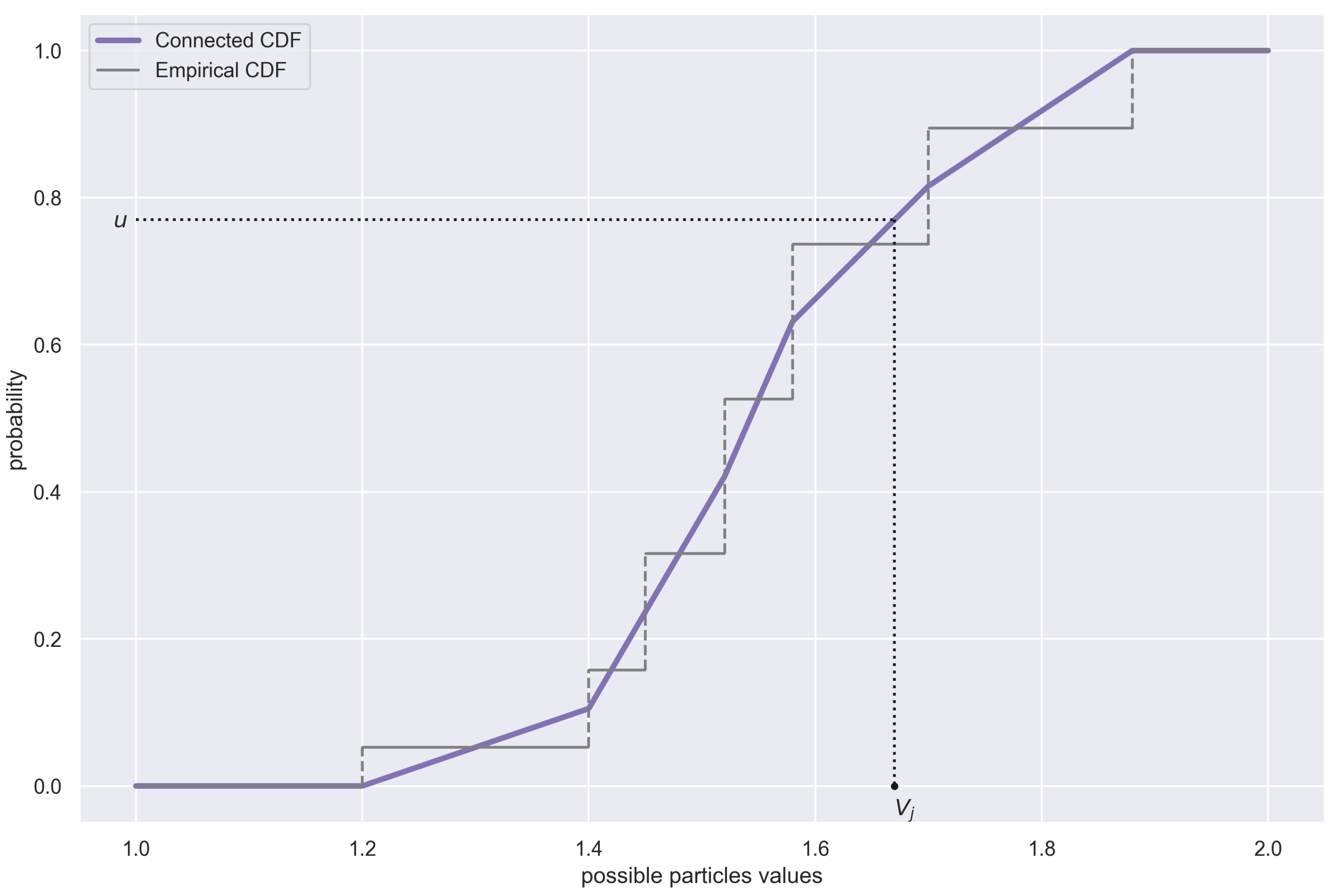
3.1.4. Estimation of —Particle Filtering
- The particle with the smallest value is the first in the new sequence, i.e.,
- The particle with the largest value is the last in the new sequence, i.e.,
- For any , we have
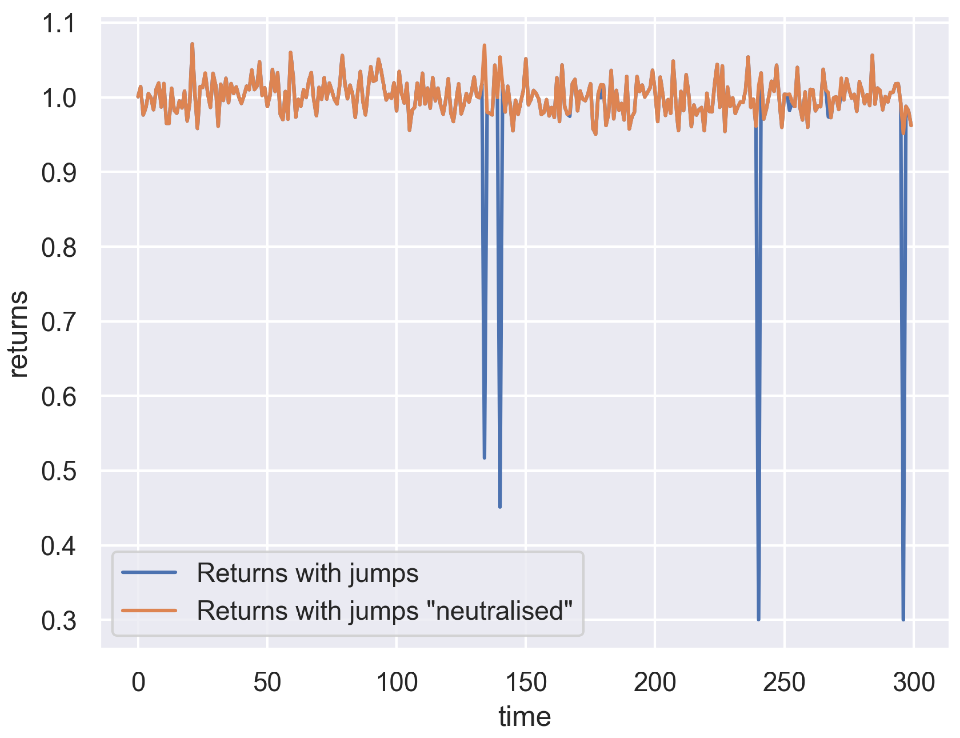
3.2. Heston Model with Jumps
3.3. Estimation Procedure
| Algorithm 1:Estimating the Heston model |
Require:
|
| Algorithm 2:Estimating the Heston model with jumps |
Require:
|
4. Analysis of the Estimation Results
4.1. Exemplary Estimation
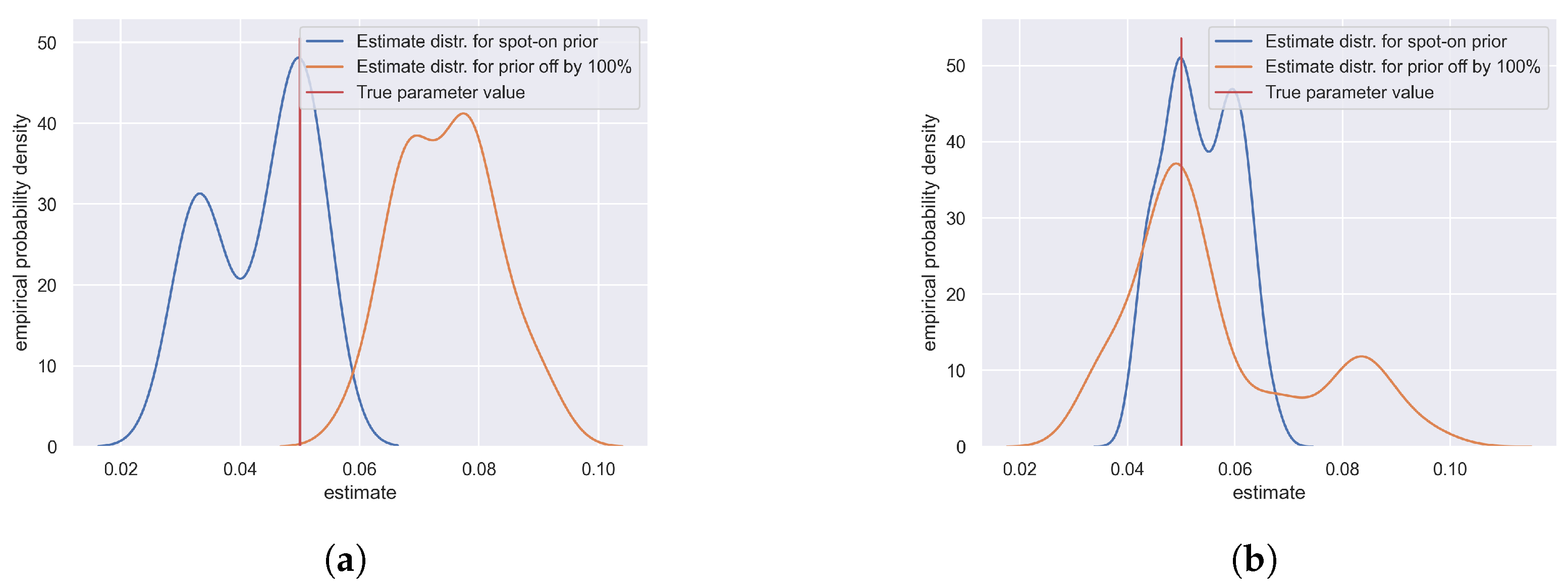
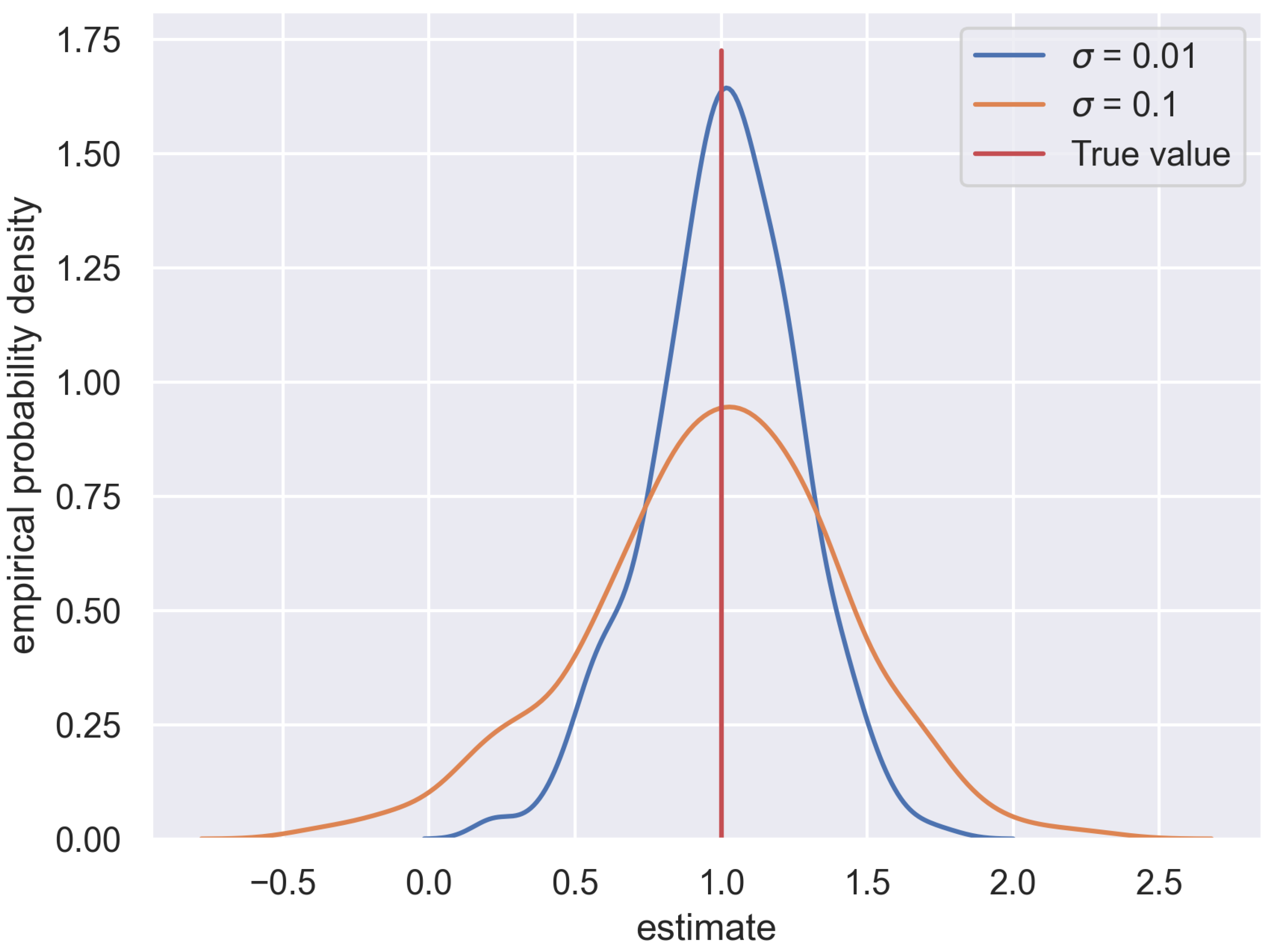
4.2. Important Findings
4.3. Towards Real-Life Applications
5. Conclusions
Author Contributions
Funding
Data Availability Statement
Conflicts of Interest
Appendix A. Table of Symbols

| Quantity | Explanation |
|---|---|
| T | max time (i.e., ) |
| asset price (with ) | |
| volatility (with ) | |
| Brownian motion for the price process | |
| Brownian motion for the volatility process | |
| drift | |
| rate of return to the long-time average | |
| long-time average | |
| volatility of the volatility | |
| correlation between prices and volatility | |
| size of the jump | |
| mean of the jump size | |
| standard deviation of the jump size | |
| Poisson process counting jumps | |
| intensity of jumps | |
| time step (also known as the discretisation constant) | |
| n | number of time steps (also known as the length of data) |
| price process random component | |
| volatility process random component | |
| additional random component—see Equation (10)) | |
| regression parameter for drift estimation—see Equation (11) | |
| ratio between neighbouring prices—see Equations (12) and (84) | |
| series of dependent variables for the drift estimation—see Equation (14) | |
| series of independent variables for the drift estimation—see Equation (15) | |
| vector of the dependent variable for the drift estimation—see Equation (17) | |
| vector of the independent variable for the drift estimation—see Equation (18) | |
| mean of the prior distribution of | |
| standard deviation of the prior distribution of |
| Quantity | Explanation |
|---|---|
| precision of the prior distribution of | |
| OLS estimator of —see (21) | |
| mean of the posterior distribution of —see (20) | |
| precision of the posterior distribution of —see (19) | |
| i-th sample of —see (22) | |
| i-th estimate of the drift—see (23) | |
| regression parameter for volatility parameters estimation—see Equation (25) | |
| regression parameter for volatility parameters estimation—see Equation (26) | |
| vector of regression parameters for volatility parameters estimation—see Equation (29) | |
| vector of the dependent variable for the volatility parameter estimation—see Equation (30) | |
| vector of the independent variable for the volatility parameter estimation—see Equation (31) | |
| vector of the independent variable for the volatility parameter estimation—see Equation (32) | |
| matrix of the independent variable for the volatility parameter estimation—see Equation (34) | |
| noise vector of the volatility parameter estimation—see Equation (35) | |
| mean vector of the prior distribution of | |
| precision matrix of the prior distribution of | |
| mean vector of the posterior distribution of —see Equation (37) | |
| precision matrix of the posterior distribution of —see (36) | |
| OLS estimator of —see (38) | |
| i-th sample of —see (39) | |
| i-th estimate of —see (40) | |
| i-th estimate of —see (41) | |
| shape parameter of the prior distribution of | |
| scale parameter of the prior distribution of | |
| shape parameter of the posterior distribution of | |
| scale parameter of the posterior distribution of | |
| i-th estimate of the —see (42) | |
| series of residuals of the price equation—see (45) | |
| series of residuals of the volatility equation—see (46) | |
| regression parameter for estimation, —see (47) | |
| regression parameter for estimation, —see (47) | |
| series of independent variables for the estimation of —see (45) | |
| series of dependent variables for the estimation of —see (46) | |
| vector of the independent variables for the estimation of —see (50) | |
| vector of the dependent variables for the estimation of —see (51) | |
| matrix of residuals—see (52) | |
| auxiliary matrix for solving regression—see (53) | |
| mean of the prior distribution of | |
| precision of the prior distribution of | |
| mean of the posterior distribution of —see (54) | |
| precision of the posterior distribution of —see (55) | |
| shape parameter of the prior distribution of | |
| scale parameter of the prior distribution of | |
| shape parameter of the posterior distribution of —see (56) | |
| scale parameter of the posterior distribution of —see (57) | |
| i-th sample of —see (59) | |
| i-th sample of —see (58) | |
| j-th sample of particle filtering independent errors—see (61) | |
| j-th sample of particle filtering residuals—see (62) | |
| j-th sample of particle filtering correlated—see (62) | |
| j-th raw volatility particle—see (64) | |
| j-th particle likelihood measure—see (65) and (77) | |
| j-th particle probability—see (66) | |
| j-th particle-probability vector—see (67) | |
| j-th raw volatility particle in a sorted sequence—see (68), (69), and (70) | |
| probability of the j-th particle in the sorted sequence—see (71) | |
| continuous CDF of resampled particles—see (72) |
| Quantity | Explanation |
|---|---|
| j-th final volatility particle—see (73) | |
| proportion of particles encoding a jump | |
| j-th raw moment-of-a-jump particle—see (75) | |
| mean of the raw size-of-a-jump particle | |
| standard deviation of the raw size-of-a-jump particle | |
| j-th raw size-of-a-jump particle—see (76) | |
| j-th resampled size-of-a-jump particle—see (78) | |
| probability of a jump—see (79) | |
| i-th estimate of —see (80) | |
| estimate of an average size of a jump—see (81) | |
| i-th estimate of —see (82) | |
| i-th estimate of —see (83) |
| 1 | Equation (65) is the reason we cannot run this procedure for , as we would not be able to obtain , since the last available value is . |
| 2 | For applications in finance, this task is sometimes easier than for some other fields of science, as numerous works have been published already, presenting the results of the estimates of well-known stocks or market indices within various models. See, e.g., Eraker et al. (2003) |
References
- Bates, David S. 1996. Jumps and Stochastic Volatility: Exchange Rate Processes Implicit in Deutsche Mark Options. The Review of Financial Studies 9: 69–107. [Google Scholar] [CrossRef]
- Black, Fischer, and Myron Scholes. 1973. The Pricing of Options and Corporate Liabilities. Journal of Political Economy 81: 637–54. [Google Scholar] [CrossRef]
- Chib, Siddhartha, and Edward Greenberg. 1995. Understanding the Metropolis-Hastings Algorithm. The American Statistician 49: 327–35. [Google Scholar] [CrossRef]
- Christoffersen, Peter, Kris Jacobs, and Karim Mimouni. 2007. Volatility Dynamics for the S&P500: Evidence from Realized Volatility, Daily Returns and Option Prices. Rochester: Social Science Research Network. [Google Scholar] [CrossRef]
- Cox, John C., Jonathan E. Ingersoll, and Stephen A. Ross. 1985. A Theory of the Term Structure of Interest Rates. Econometrica 53: 385–407. [Google Scholar] [CrossRef]
- Doucet, Arnaud, and Adam Johansen. 2009. A Tutorial on Particle Filtering and Smoothing: Fifteen Years Later. Handbook of Nonlinear Filtering 12: 3. [Google Scholar]
- Eraker, Bjørn, Michael Johannes, and Nicholas Polson. 2003. The Impact of Jumps in Volatility and Returns. The Journal of Finance 58: 1269–300. [Google Scholar] [CrossRef]
- Gruszka, Jarosław, and Janusz Szwabiński. 2021. Advanced strategies of portfolio management in the Heston market model. Physica A: Statistical Mechanics and Its Applications 574: 125978. [Google Scholar] [CrossRef]
- Gruszka, Jarosław, and Janusz Szwabiński. 2023. Portfolio optimisation via the heston model calibrated to real asset data. arXiv arXiv:2302.01816. [Google Scholar]
- Heston, Steven. 1993. A Closed-Form Solution for Options with Stochastic Volatility with Applications to Bond and Currency Options. The Review of Financial Studies 6: 327–43. [Google Scholar] [CrossRef]
- Jacquier, Eric, Nicholas G. Polson, and Peter E. Rossi. 2004. Bayesian analysis of stochastic volatility models with fat-tails and correlated errors. Journal of Econometrics 122: 185–212. [Google Scholar] [CrossRef]
- Johannes, Michael, and Nicholas Polson. 2010. CHAPTER 13—MCMC Methods for Continuous-Time Financial Econometrics. In Handbook of Financial Econometrics: Applications. Edited by Yacine Aït-Sahalia and Lars Peter Hansen. San Diego: Elsevier, vol. 2, pp. 1–72. [Google Scholar] [CrossRef]
- Johannes, Michael, Nicholas Polson, and Jonathan Stroud. 2009. Optimal Filtering of Jump Diffusions: Extracting Latent States from Asset Prices. Review of Financial Studies 22: 2559–99. [Google Scholar] [CrossRef]
- Kloeden, Peter, and Eckhard Platen. 1992. Numerical Solution of Stochastic Differential Equations, 1st ed. Stochastic Modelling and Applied Probability. Berlin/Heidelberg: Springer. [Google Scholar]
- Lindley, Dennis. V., and Adrian F. M. Smith. 1972. Bayes Estimates for the Linear Model. Journal of the Royal Statistical Society: Series B (Methodological) 34: 1–18. [Google Scholar] [CrossRef]
- Meissner, Gunter, and Noriko Kawano. 2001. Capturing the volatility smile of options on high-tech stocks—A combined GARCH-neural network approach. Journal of Economics and Finance 25: 276–92. [Google Scholar] [CrossRef]
- O’Hagan, Anthony, and Maurice George Kendall. 1994. Kendall’s Advanced Theory of Statistics: Bayesian Inference. Volume 2B. London: Arnold. [Google Scholar]
- Wong, Bernard, and Chris C. Heyde. 2006. On changes of measure in stochastic volatility models. International Journal of Stochastic Analysis 2006: 018130. [Google Scholar] [CrossRef]


| Prior Parameter | Value |
|---|---|
| 1.00125 | |
| 0.001 | |
| 149 | |
| 0.025 | |
| 0.3 | |
| 1.03 | |
| 0.05 | |
| 0.15 | |
| 0.3 |
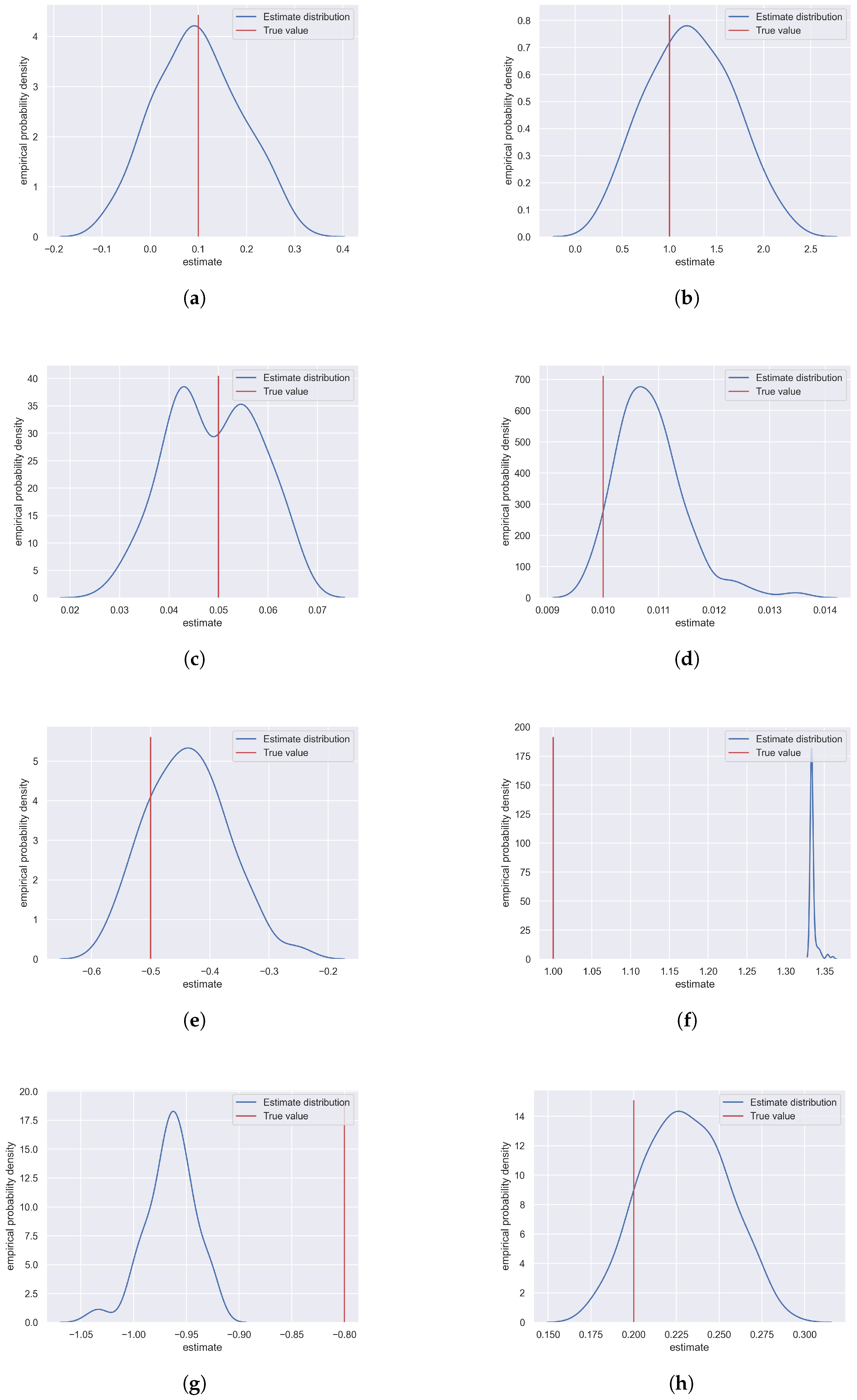
| Parameter | True Value | Estimated Value | Relative Error [%] |
|---|---|---|---|
| 0.1 | 0.09829 | 1.77 | |
| 1 | 1.2190 | 21.90 | |
| 0.05 | 0.0493 | 1.92 | |
| 0.01 | 0.0108 | 8.55 | |
| −0.5 | 0.4379 | 12.40 | |
| 1 | 1.3349 | 33.49 | |
| −0.8 | −0.9651 | 20.64 | |
| 0.2 | 0.2298 | 14.88 |
Disclaimer/Publisher’s Note: The statements, opinions and data contained in all publications are solely those of the individual author(s) and contributor(s) and not of MDPI and/or the editor(s). MDPI and/or the editor(s) disclaim responsibility for any injury to people or property resulting from any ideas, methods, instructions or products referred to in the content. |
© 2023 by the authors. Licensee MDPI, Basel, Switzerland. This article is an open access article distributed under the terms and conditions of the Creative Commons Attribution (CC BY) license (https://creativecommons.org/licenses/by/4.0/).
Share and Cite
Gruszka , J.; Szwabiński, J. Parameter Estimation of the Heston Volatility Model with Jumps in the Asset Prices. Econometrics 2023, 11, 15. https://doi.org/10.3390/econometrics11020015
Gruszka J, Szwabiński J. Parameter Estimation of the Heston Volatility Model with Jumps in the Asset Prices. Econometrics. 2023; 11(2):15. https://doi.org/10.3390/econometrics11020015
Chicago/Turabian StyleGruszka , Jarosław, and Janusz Szwabiński. 2023. "Parameter Estimation of the Heston Volatility Model with Jumps in the Asset Prices" Econometrics 11, no. 2: 15. https://doi.org/10.3390/econometrics11020015
APA StyleGruszka , J., & Szwabiński, J. (2023). Parameter Estimation of the Heston Volatility Model with Jumps in the Asset Prices. Econometrics, 11(2), 15. https://doi.org/10.3390/econometrics11020015