Causal Vector Autoregression Enhanced with Covariance and Order Selection

Abstract

A causal vector autoregressive (CVAR) model is introduced for weakly stationary multivariate processes, combining a recursive directed graphical model for the contemporaneous components and a vector autoregressive model longitudinally. Block Cholesky decomposition with varying block sizes is used to solve the model equations and estimate the path coefficients along a directed acyclic graph (DAG). If the DAG is decomposable, i.e., the zeros form a reducible zero pattern (RZP) in its adjacency matrix, then covariance selection is applied that assigns zeros to the corresponding path coefficients. Real-life applications are also considered, where for the optimal order $p\ge 1$ of the fitted CVAR$\left(p\right)$ model, order selection is performed with various information criteria.

1. Introduction

The purpose of the present paper is to connect graphical modeling tools and time series models together via path coefficient estimation. In statistics, the path analysis was established by the geneticist Wright (1934) about a century ago, but he used complicated entrywise calculations with partial correlations. Taking these partial correlations of a pair of variables in a multidimensional data set conditioned on another set of variables makes things overtly complicated, as the conditioning set changes in the steps. A bit later, in econometrics, structural equation modeling (SEM) was developed; the prominent author Haavelmo (1943) obtained the Nobel price for it later. The maximum likelihood estimation (MLE) of the parameters in the Gaussian case was elaborated by Joreskog (1977). At the same time, Ref. Wold (1985), the inventor of partial least squares regression (PLS), used matrix calculations, and Ref. Kiiveri et al. (1984) already used block matrix decompositions when dividing their variables into endogenous and exogenous ones. However, none of these authors applied steadily algorithms of block LDL (variant of the Cholesky) decomposition alone, without using partial correlations. Furthermore, they did not consider time series.

Here, we give a rigorous block matrix approach of these problems that originated in statistics and time series analysis. Furthermore, we enhance the usual and structural vector autoregressive (VAR and SVAR) models, discussed e.g., in Deistler and Scherrer (2019) and Deistler and Scherrer (2022), with a causal component that has an effect between the coordinates contemporaneously. Therefore, we call our causal vector autoregressive model CVAR. Joint effects between the contemporaneous components are also considered in SVAR models of Keating (1996); Lütkepohl (2005); and Kilian and Lütkepohl (2017), but just recursive ordering of the variables, and no specific structure of the underlying directed graph is investigated. Though in Wold (1960) a causal chain model is introduced with an exogenous and a lagged endogenous variable, Gaussian Markov processes and usual regression estimates are used in the context of econometric problems. This research is also inspired by the paper Wermuth (1980), where recursive ordering of the variables is crucial, without using any time component.

Ref. Eichler (2006) introduces causality as a fundamental tool for the empirical investigations of dynamic interactions in multivariate time series. He also discusses the differences between the structural and Granger causality. The former one appears in the SVAR models (see Geweke (1984)), whereas the latter one first appears in Wiener (1956), then in Granger (1969), and is sometimes called Wiener–Granger causality. Without causality between the contemporaneous components, our model in the Gaussian case also resembles the one of Eichler (2012), where the error term (shock) can have correlated components. Our higher order recursive VAR model can be transformed into a model like this, but the price is losing the recursive structure. The VAR model of Brillinger (1996) has a similar structure as ours with uncorrelated error terms; but no further benefits of recursive models, such as RZP, induced by the underlying DAG, are discussed. Ref. Sims (1980) investigates the use of different types of structural equations and autoregressive models in macroeconomics, without suggesting numerical algorithms. However, historically, this survey paper was among the first ones which pointed out the difference between the existing macroeconomic models so far and distinguished endogenous and exogenous variables. The method of the most recent paper Bazinas and Nielsen (2022) is based on the reduced form system and is constructed by the conditional distribution of two endogenous variables, given a catalyst or multiple catalysts; lagged effects are assessed, without having a longer time series, and stationarity is not assumed.

Throughout the paper, second order processes are considered that can be assumed to asymptotically follow multivariate Gaussian distribution. In Section 2, the different types of VAR models are compared, and a novel CVAR model is introduced, combining a recursive graphical model contemporaneously and a VAR$\left(p\right)$ model longitudinally. In Section 3, the models are described in details, together with introducing algorithms for the parameter estimation. In Section 3.1, the unrestricted CVAR$\left(p\right)$ model is introduced, while in Section 3.2, the restricted cases are treated, with some prescribed zeros in the path coefficients. Relation to covariance selection and decomposability is discussed too. In Section 4, application to real life data is presented together with information criteria for order selection (optimal choice of p). The results and estimation schemes are summarized in Section 5; finally, in Section 6, conclusions and further perspectives are posed. The proofs of the theorems and the detailed description of the algorithms are to be found in Appendix A, while the pseudocodes in Appendix B. To illustrate the CVAR model and related algorithms, there are supporting Python files and notebooks uploaded, together with some additional tables and figures. These are included in the Supplementary Material.

2. Materials and Methods

First, the different purpose VAR$\left(p\right)$ models for the d-dimensional, weakly stationary process $\left\{{\mathbf{X}}_t\right\}$ are enlisted and compared. The first two models are known in the literature, whereas the last two are our contributions, for which block matrix decomposition based algorithms are introduced in Section 3, and they are illustrated in Section 4 on real life data.

• Reduced form VAR$\left(p\right)$ model: for given integer $p\ge 1$, it is

  $${\mathbf{X}}_t+{\mathit{M}}_1{\mathbf{X}}_{t-1}+\cdots +{\mathit{M}}_p{\mathbf{X}}_{t-p}={\mathbf{V}}_t,t=p+1,p+2,\dots ,$$

  (1)

  where ${\mathbf{V}}_t$ is white noise, it is uncorrelated with ${\mathbf{X}}_{t-1},\dots ,{\mathbf{X}}_{t-p}$, it has zero expectation and covariance matrix $\mathsf{\Sigma }$ (not necessarily diagonal, but positive definite), and the matrices ${\mathit{M}}_j$ satisfy the stability conditions (see Deistler and Scherrer (2019)). (Sometimes, ${\mathbf{X}}_t$ is isolated on the left-hand side.) ${\mathbf{V}}_t$ is called innovation, i.e., the error term of the (added value to the) best one-step ahead linear prediction of ${\mathbf{X}}_t$ with its past, which (in the case of a VAR(p) model) can be carried out with the p-lag long past ${\mathbf{X}}_{t-1},\dots ,{\mathbf{X}}_{t-p}$.
  Here, the ordering of the components of ${\mathbf{X}}_t$ does not matter: if it is changed (with some permutation of $\{1,\dots ,d\}$), then clearly the rows of the matrices ${\mathit{M}}_j$s and, furthermore, the rows and columns of $\mathsf{\Sigma }$ are permuted accordingly.
• Structural form SVAR$\left(p\right)$ model: for given integer $p\ge 1$, it is

  $$\mathit{A}{\mathbf{X}}_t+{\mathit{B}}_1{\mathbf{X}}_{t-1}+\cdots +{\mathit{B}}_p{\mathbf{X}}_{t-p}={\mathbf{U}}_t,t=p+1,p+2,\dots ,$$

  (2)

  where the white noise term ${\mathbf{U}}_t$ is uncorrelated with ${\mathbf{X}}_{t-1},\dots ,{\mathbf{X}}_{t-p}$, and it has zero expectation with uncorrelated components, i.e., with positive definite, diagonal covariance matrix $\Delta$. $\mathit{A}$ is a $d\times d$ upper triangular matrix with 1s along its main diagonal, whereas ${\mathit{B}}_1,\dots ,{\mathit{B}}_p$ are $d\times d$ matrices; see also Lütkepohl (2005). The components of ${\mathbf{U}}_t$ are called structural shocks, and they are mutually uncorrelated and assigned to the individual variables.
  Here, the ordering of the components of ${\mathbf{X}}_t$ does matter: if it is changed (with some permutation of $\{1,\dots ,d\}$), then the matrices $\mathit{A}$, ${\mathit{B}}_j$ and $\Delta$ cannot be obtained in a simple way; they profoundly change under the given permutation.
  However, there is a one-to-one correspondence between the reduced and structural model; since $\mathit{A}$ is invertible, from Equation (2), Equation (1) can be obtained (and vice versa):

  $${\mathbf{X}}_t+{\mathit{A}}^{-1}{\mathit{B}}_1{\mathbf{X}}_{t-1}+\cdots +{\mathit{A}}^{-1}{\mathit{B}}_p{\mathbf{X}}_{t-p}={\mathit{A}}^{-1}{\mathbf{U}}_t,t=p+1,p+2,\dots ,$$

  where ${\mathit{M}}_j={\mathit{A}}^{-1}{\mathit{B}}_j$, ${\mathbf{V}}_t={\mathit{A}}^{-1}{\mathbf{U}}_t$, and $\mathsf{\Sigma }={\mathit{A}}^{-1}\Delta {{\mathit{A}}^T}^{-1}$; further, $\left|\mathsf{\Sigma }\right|=|\Delta |$ as $\left|\mathit{A}\right|=1$.
• Causal CVAR$\left(p\right)$ unrestricted model: it also obeys Equation (2), but here the ordering of the components follows a causal ordering, given e.g., by an expert’s knowledge. This is a recursive ordering along a “complete” DAG, where the permutation (labeling) of the graph nodes (assigned to the components of ${\mathbf{X}}_t$) is such that $X_{t,i}$ can be caused by $X_{t,j}$ whenever $i<j$, which means a $j\to i$ directed edge. Here, the causal effects are meant contemporaneously, and reflected by the upper triangular structure of the matrix $\mathit{A}$.
  It is important that, in any ordering of the jointly Gaussian variables, a Bayesian network (in other words, a Gaussian directed graphical model) can be constructed, in which every node (variable) is regressed linearly with the variables corresponding to higher label nodes. The partial regression coefficients behave like path coefficients, also used in SEM. If the DAG is complete, then there are no zero constraints imposed on the partial regression coefficients. Here, building the DAG just aims at finding a sensible ordering of the variables.
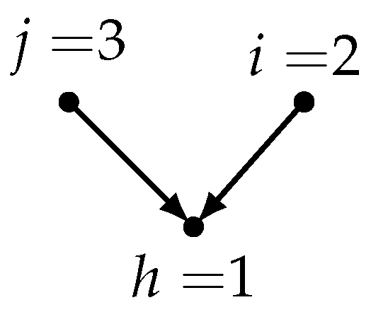
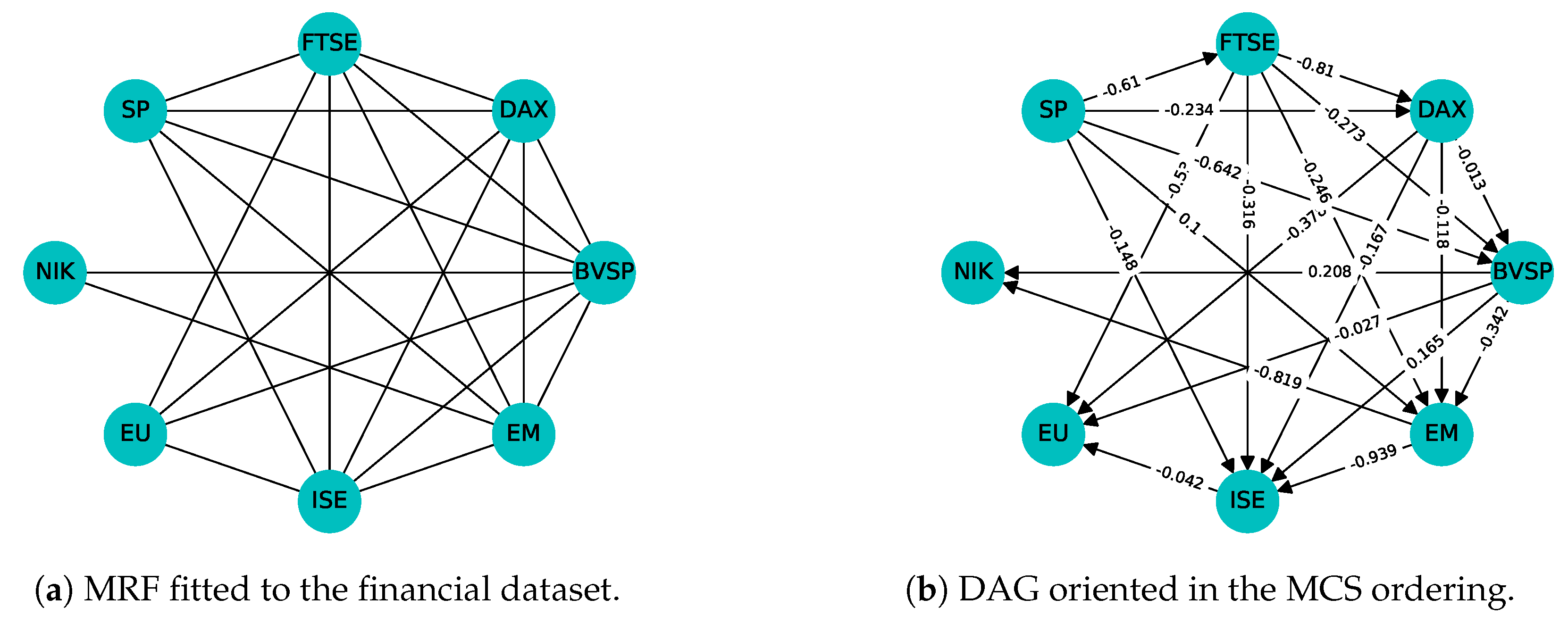
• Causal CVAR$\left(p\right)$ restricted model: here, an incomplete DAG is built, based on partial correlations.
  First, we build an undirected graph: do not connect i and j if the partial correlation coefficients of $X_i$ and $X_j$, eliminating the effect of the other variables is 0 (theoretically), or less than a threshold (practically). Such an undirected graphical model is called Markov random field (MRF). It is known (see Rao (1973) and Lauritzen (2004)) that partial correlations can be calculated from the concentration matrix (inverse of the covariance matrix). However, here the upper left block of the inverse of the large block matrix, containing the first p autocovariance matrices, is used. If this undirected graph is triangulated, then in a convenient (so-called perfect) ordering of the nodes, the zeros of the adjacency matrix form an RZP. We can find such a (not necessarily unique) ordering of the nodes with the maximal cardinality search (MCS) algorithm, together with cliques and separators of a so-called junction tree (JT); see Lauritzen (2004), Koller and Friedman (2009), and Bolla et al. (2019). In this ordering (labeling) of the nodes, a DAG can also be constructed, which is Markov equivalent to the undirected one (it has no so-called sink V configuration); for further details, see Section 3.2.
  Having an RZP in the CVAR restricted model, we use the incomplete DAG for estimation. With the covariance selection method of Dempster (1972), the starting concentration matrix is re-estimated by imposing zero constraints for its entries in the RZP positions (symmetrically). By the theory (see, e.g., Bolla et al. (2019)), this will result in zero entries of $\mathit{A}$ in the no directed edge positions.

Note that the unrestricted CVAR model can use an incomplete DAG as well, where the labeling of its nodes follows the perfect labeling of the undirected graph; still, the parameter matrices $\mathit{A}$ and ${\mathit{B}}_j$s are “full” in the sense that no zeros of $\mathit{A}$ are guaranteed in the no-edge positions of the graph. Their entries are just considered as path coefficients of the contemporaneous and lagged effects, respectively. On the contrary, in the restricted CVAR model, action is carried out for introducing zero entries in $\mathit{A}$ in the no-edge positions. If the desired zeros form an RZP, the covariance selection has a closed form (see Lauritzen (2004)). In the lack of an RZP, the covariance selection still works, but it needs an infinite (convergent) iteration, called iterative proportional scaling (IPS), see Lauritzen (2004) and Bolla et al. (2019). Other possibility is to moralize the DAG (connect parents that are not connected and thus eliminate the sink Vs), and work with the so-obtained undirected graph.

Then, both in the unrestricted and restricted CVAR$\left(p\right)$ models, an order selection is initiated to choose the optimal p, based on information criteria, such as AIC, BIC, AICC, and HQ, where only the number of parameters differs in the two cases. Actually, in the restricted case, the product-moments are calculated only within the cliques, and since separators are subsets of them, we can reduce the computational complexity of our algorithm that is spectacular when the number of nodes is “large”.

3. Results

3.1. The Unrestricted Causal VAR(p) Model

The directed Gaussian graphical model of Wermuth (1980) does not consider time development; it is, in fact, a CVAR(0) model. In addition, note that at this point, the ordering of the jointly Gaussian variables is not relevant, since in any recursive ordering of them (encoded in $\mathit{A}$), a Gaussian directed graphical model (in other words, a Gaussian Bayesian network) can be constructed, where every variable is regressed linearly with the higher label ones.

To illustrate the $p>0$ case, first we introduce the unrestricted CVAR(1) model. This has a special interest, as can be used for longitudinal data spanning a short time interval or adapted to the situation when ${\mathbf{X}}_{t-1}$ represents the exogenous, and ${\mathbf{X}}_t$ the endogenous variables in their components.

Let $\left\{{\mathbf{X}}_t\right\}$ be a d-dimensional, weakly stationary process with real valued components of zero expectation and covariance matrix function $\mathit{C}\left(h\right)$, $h=0,\pm 1,\pm 2,\dots$; $\mathit{C}(-h)={\mathit{C}}^T\left(h\right)$. All deterministic and random vectors are column vectors and so $\mathit{C}\left(h\right)=\mathbb{E}{\mathbf{X}}_t{\mathbf{X}}_{t+h}^T$ does not depend on t, by weak stationarity. The CVAR(1) model equation is

$$\mathit{A}{\mathbf{X}}_t+\mathit{B}{\mathbf{X}}_{t-1}={\mathbf{U}}_t,t=1,2,\dots ,$$

(3)

where $\mathit{A}$ is a $d\times d$ upper triangular matrix with 1s along its main diagonal, $\mathit{B}$ is a $d\times d$ matrix; furthermore, the white noise random vector ${\mathbf{U}}_t$ is uncorrelated with (in the Gaussian case, independent of) ${\mathbf{X}}_{t-1}$, has zero expectation, and covariance matrix $\Delta =\mathrm{diag}({\delta }_1,\dots ,{\delta }_d)$.

Let ${\mathfrak{C}}_2$ denote the covariance matrix of the stacked random vector ${({\mathbf{X}}_t^T,{\mathbf{X}}_{t-1}^T)}^T$ which, in block matrix form, is as follows:

$${\mathfrak{C}}_2=\left(\begin{array}{cc}\mathit{C}\left(0\right)& {\mathit{C}}^T\left(1\right)\\ \mathit{C}\left(1\right)& \mathit{C}\left(0\right)\end{array}\right).$$

(4)

It is symmetric and positive definite if the process is of full rank regular (which means that its spectral density matrix is of full rank, see Bolla and Szabados (2021)) that is assumed in the sequel. It is well known that the inverse of ${\mathfrak{C}}_2$, the so-called concentration matrix $\mathit{K}$, has the block-matrix form

$$\mathit{K}=\left(\begin{array}{cc}{\mathit{C}}^{-1}\left(1\right|0)& -{\mathit{C}}^{-1}\left(1\right|0){\mathit{C}}^T\left(1\right){\mathit{C}}^{-1}\left(0\right)\\ -{\mathit{C}}^{-1}\left(0\right)\mathit{C}\left(1\right){\mathit{C}}^{-1}\left(1\right|0)& {\mathit{C}}^{-1}\left(0\right)+{\mathit{C}}^{-1}\left(0\right)\mathit{C}\left(1\right){\mathit{C}}^{-1}\left(1\right|0){\mathit{C}}^T\left(1\right){\mathit{C}}^{-1}\left(0\right)\end{array}\right),$$

where $\mathit{C}\left(1\right|0)=\mathit{C}\left(0\right)-{\mathit{C}}^T\left(1\right){\mathit{C}}^{-1}\left(0\right)\mathit{C}\left(1\right)$ is the conditional covariance matrix $\mathit{C}\left(t\right|t-1)$ of the distribution of ${\mathbf{X}}_t$, given ${\mathbf{X}}_{t-1}$; by weak stationarity, it does not depend on t either; therefore, it is denoted by $\mathit{C}\left(1\right|0)$. In addition, ${\mathfrak{C}}_2$ is positive definite if and only if both $\mathit{C}\left(0\right)$ and $\mathit{C}\left(1\right|0)$ are positive definite.

Observe that $\mathit{C}\left(1\right|0)={\mathit{A}}^{-1}\Delta {{\mathit{A}}^{-1}}^T$ is the covariance matrix of the innovation ${\mathbf{V}}_t={\mathit{A}}^{-1}{\mathbf{U}}_t$. Therefore, the left upper block of $\mathit{K}$ contains its inverse, which is ${\mathit{A}}^T{\Delta }^{-1}\mathit{A}$.

Theorem 1.

The parameter matrices $\mathit{A}$, $\mathit{B}$, and $\Delta$ of model Equation (3) can be obtained by the block LDL decomposition of the (positive definite) concentration matrix $\mathit{K}$ (inverse of the covariance matrix ${\mathfrak{C}}_2$ in Equation (4)) of the $2d$-dimensional Gaussian random vector ${({\mathbf{X}}_t^T,{\mathbf{X}}_{t-1}^T)}^T$. If $\mathit{K}=\mathit{L}\mathit{D}{\mathit{L}}^T$ is this (unique) decomposition with block-triangular matrix $\mathit{L}$ and block-diagonal matrix $\mathit{D}$, then they have the form

$$\mathit{L}=\left(\begin{array}{cc}{\mathit{A}}^T& {\mathit{O}}_{d\times d}\\ {\mathit{B}}^T& {\mathit{I}}_{d\times d}\end{array}\right),\hspace{1em}\hspace{1em}\mathit{D}=\left(\begin{array}{cc}{\Delta }^{-1}& {\mathit{O}}_{d\times d}\\ {\mathit{O}}_{d\times d}& {\mathit{C}}^{-1}\left(0\right)\end{array}\right),$$

(5)

where the $d\times d$ upper triangular matrix $\mathit{A}$ with 1s along its main diagonal, the $d\times d$ matrix $\mathit{B}$, and the diagonal matrix $\Delta$ of model Equation (3) can be retrieved from them.

The proof of this theorem together with the detailed description of the algorithm is to be found in Appendix A.1 and Appendix A.2 of Appendix A.

The above model naturally generalizes to the following recursive CVAR(p) model: for given integer $p\ge 1$,

$$\mathit{A}{\mathbf{X}}_t+{\mathit{B}}_1{\mathbf{X}}_{t-1}+\dots +{\mathit{B}}_p{\mathbf{X}}_{t-p}={\mathbf{U}}_t,t=p+1,p+2,\dots ,$$

(6)

where the white noise term ${\mathbf{U}}_t$ is uncorrelated with ${\mathbf{X}}_{t-1},\dots ,{\mathbf{X}}_{t-p}$, it has zero expectation and covariance matrix $\Delta =\mathrm{diag}({\delta }_1,\dots ,{\delta }_d)$. $\mathit{A}$ is a $d\times d$ upper triangular matrix with 1s along its main diagonal; whereas, ${\mathit{B}}_1,\dots ,{\mathit{B}}_p$ are $d\times d$ matrices.

Here, we have to perform the block Cholesky decomposition of the inverse covariance matrix of ${({\mathbf{X}}_t^T,{\mathbf{X}}_{t-1}^T,\dots ,{\mathbf{X}}_{t-p}^T)}^T$, i.e., the inverse of the matrix

$${\mathfrak{C}}_{p+1}=\left(\begin{array}{ccccc}\mathit{C}\left(0\right)\hfill & {\mathit{C}}^T\left(1\right)\hfill & {\mathit{C}}^T\left(2\right)\hfill & \dots \hfill & {\mathit{C}}^T\left(p\right)\hfill \\ \mathit{C}\left(1\right)\hfill & \mathit{C}\left(0\right)\hfill & {\mathit{C}}^T\left(1\right)\hfill & \dots \hfill & {\mathit{C}}^T(p-1)\hfill \\ \mathit{C}\left(2\right)\hfill & \mathit{C}\left(1\right)\hfill & \mathit{C}\left(0\right)\hfill & \dots \hfill & {\mathit{C}}^T(p-2)\hfill \\ ⋮\hfill & ⋮\hfill & ⋮\hfill & \ddots \hfill & ⋮\hfill \\ \mathit{C}\left(p\right)\hfill & \mathit{C}(p-1)\hfill & \mathit{C}(p-2)\hfill & \dots \hfill & \mathit{C}\left(0\right)\hfill \end{array}\right).$$

(7)

This is a symmetric, positive definite block Toeplitz matrix with $(p+1)\times (p+1)$ blocks which are $d\times d$ matrices. Again, ${\mathit{C}}^T\left(h\right)=\mathit{C}(-h)$, and it is well known that the inverse matrix ${\mathfrak{C}}_{p+1}^{-1}$ has the following block-matrix form:

• Upper left block: ${\mathit{C}}^{-1}\left(p\right|0,\dots ,p-1)$;
• Upper right block: $-{\mathit{C}}^{-1}\left(p\right|0,\dots ,p-1){\mathit{C}}^T(1,\dots ,p){\mathfrak{C}}_p^{-1}$;
• Lower left block: $-{\mathfrak{C}}_p^{-1}\mathit{C}(1,\dots ,p){\mathit{C}}^{-1}\left(p\right|0,\dots ,p-1)$;
• Lower right block: ${\mathfrak{C}}_p^{-1}+{\mathfrak{C}}_p^{-1}\mathit{C}(1,\dots ,p){\mathit{C}}^{-1}\left(p\right|0,\dots ,p-1){\mathit{C}}^T(1,\dots ,p){\mathfrak{C}}_p^{-1}$,

where $\mathit{C}\left(p\right|0,\dots ,p-1)=\mathit{C}\left(0\right)-{\mathit{C}}^T(1,\dots ,p){\mathfrak{C}}_p^{-1}\mathit{C}(1,\dots ,p)$ is the conditional covariance matrix $\mathit{C}\left(t\right|t-1,\dots ,t-p)$ of the distribution of ${\mathbf{X}}_t$ given ${\mathbf{X}}_{t-1},\dots ,{\mathbf{X}}_{t-p}$; due to stationarity, it does not depend on t either; therefore, it is denoted by $\mathit{C}\left(p\right|0,\dots ,p-1)$. Furthermore, ${\mathit{C}}^T(1,\dots ,p)=({\mathit{C}}^T\left(1\right),\dots ,{\mathit{C}}^T\left(p\right))$ is a $d\times pd$ and $\mathit{C}(1,\dots ,p)$ is a $pd\times d$ matrix. In addition, ${\mathfrak{C}}_{p+1}$ is positive definite if and only if both ${\mathfrak{C}}_p$ and $\mathit{C}\left(p\right|0,\dots ,p-1)$ are positive definite.

Theorem 2.

The parameter matrices $\mathit{A}$, ${\mathit{B}}_1,\dots ,{\mathit{B}}_p$ and $\Delta$ of model Equation (6) can be obtained by the block LDL decomposition of the (positive definite) concentration matrix $\mathit{K}$ (inverse of the covariance matrix ${\mathfrak{C}}_{p+1}$ in Equation (7)) of the $(p+1)d$-dimensional Gaussian random vector ${({\mathbf{X}}_t^T,{\mathbf{X}}_{t-1}^T,\dots ,{\mathbf{X}}_{t-p}^T)}^T$. If $\mathit{K}=\mathit{L}\mathit{D}{\mathit{L}}^T$ is this (unique) decomposition with block-triangular matrix $\mathit{L}$ and block-diagonal matrix $\mathit{D}$, then they have the form

$$\mathit{L}=\left(\begin{array}{cc}{\mathit{A}}^T& {\mathit{O}}_{d\times pd}\\ {\mathit{B}}^T& {\mathit{I}}_{pd\times pd}\end{array}\right),\mathit{D}=\left(\begin{array}{cc}{\Delta }^{-1}& {\mathit{O}}_{d\times pd}\\ {\mathit{O}}_{pd\times d}& {\mathfrak{C}}_p^{-1},\end{array}\right)$$

(8)

where the $d\times d$ upper triangular matrix $\mathit{A}$ with 1s along its main diagonal, the $d\times pd$ matrix $\mathit{B}=({\mathit{B}}_1\dots {\mathit{B}}_p)$ (transpose of ${\mathit{B}}^T$, partitioned into blocks) and the diagonal matrix $\Delta$ of model Equation (6) can be retrieved from them.

The proof of this theorem together with the detailed description of the algorithm is to be found in Appendix A.3 and Appendix A.4 of Appendix A.

3.2. The Restricted Causal VAR(p) Model

First, we again consider the $p=1$ case. Assume that we have a causal ordering of the coordinates $X_1,\dots ,X_d$ of $\mathbf{X}$ such that $X_j$ can be the cause of $X_i$ whenever $i<j$. We can think of $X_i$s as the nodes of a graph in a directed graphical model (Bayesian network) and their labeling corresponds to a topological ordering of the nodes in the underlying DAG. Thus, $i<j$ can imply a $j\to i$ edge, and then we say that $X_j$ is a parent (cause) of $X_i$. ($X_i$ can have multiple parents, maximum $d_i$ ones.) For example, when asset prices or relative returns of different assets or currencies (on the same day) influence each other in a certain (recursive) order. Now, restricted cases are analyzed, when only certain arrows (causes) are present, but the DAG is connected. In particular, only certain asset prices influence some others on a DAG contemporaneously, but not all possible directed edges are present. In this case, a covariance selection technique can be initiated to re-estimate the covariance matrix so that the partial regression coefficients in the no-edge positions are zeros.

Our DAG is sometimes given by an expert’s knowledge, but usually it is built from an undirected graph, when we also require that the so-constructed DAG be Markov equivalent to its undirected skeleton. Then, the DAG must not contain a sink V configuration. Under sink V configuration, a triplet $j\to h\leftarrow i$ is understood, where i is not connected by j$(h<i<j)$; see Figure 1.

Here, we include a short description on the relation between directed and undirected graphical models, with emphases on the Gaussian case, based on Lauritzen (2004) and Bolla et al. (2019). Directed and undirected models have many properties in common, and under some conditions, there are important correspondences between them.

Let $\mathbf{X}\sim {\mathcal{N}}_d(\mathbf{\mu },\mathsf{\Sigma })$ be a d-variate non-degenerate Gaussian random vector with expectation $\mathbf{\mu }$ and positive definite, symmetric $d\times d$ covariance matrix $\mathsf{\Sigma }$. The also positive definite, symmetric matrix ${\mathsf{\Sigma }}^{-1}$ of entries ${\sigma }^{ij}$ is called a concentration matrix, it appears in the joint density, and its zero entries indicate conditional independences between two components of $\mathbf{X}$, given the remaining ones. Mostly, the variables are already centered, so $\mathbf{\mu }=\mathbf{0}$ is assumed.

Let us form an undirected graph G on the node-set $V=\{1,\dots ,d\}$, where V corresponds to the components of $\mathbf{X}$, and the edges are drawn according to the rule

$$i\sim j\iff {\sigma }^{ij}\ne 0,i\ne j.$$

(9)

This is called an undirected Gaussian graphical model, which is a special Markov Random Field (MRF). To establish conditional independence statements, we use the following facts.

Proposition 1.

Let $\mathbf{X}={(X_1,\dots ,X_d)}^T\sim {\mathcal{N}}_d(\mathbf{0},\mathsf{\Sigma })$ be a random vector, and let $V:=\{1,\dots ,d\}$ denote the index set of the variables, $d\ge 3$. Assume that $\mathsf{\Sigma }$ is positive definite. Then,

$$r_{X_i{X}_j|{\mathbf{X}}_{V\backslash \{i,j\}}}=\frac{-{\sigma }^{ij}}{\sqrt{{\sigma }^{ii}{\sigma }^{jj}}}i\ne j,$$

where $r_{X_i{X}_j|{\mathbf{X}}_{V\backslash \{i,j\}}}$ denotes the partial correlation coefficient between $X_i$ and $X_j$ after eliminating the effect of the remaining variables ${\mathbf{X}}_{V\backslash \{i,j\}}$. Furthermore,

$${\sigma }^{ii}=1/(\mathrm{Var}\left(X_i\right|{\mathbf{X}}_{V\backslash \left\{i\right\}}),i=1,\dots ,d$$

is the reciprocal of the conditional (residual) variance of $X_i$, given the other variables ${\mathbf{X}}_{V\backslash \left\{i\right\}}$.

Definition 1.

Let $\mathbf{X}\sim {\mathcal{N}}_d(\mathbf{0},\mathsf{\Sigma })$ be a random vector with $\mathsf{\Sigma }$ positive definite. Consider the regression plane

$$\mathbb{E}\left(X_i\right|{\mathbf{X}}_{V\backslash \left\{i\right\}}={\mathbf{x}}_{V\backslash \left\{i\right\}})=\sum _{j\in V\backslash \left\{i\right\}}{\beta }_{ji·V\backslash \left\{i\right\}}{x}_j,j\in V\backslash \left\{i\right\},$$

where $x_j$’s are the coordinates of ${\mathbf{x}}_{V\backslash \left\{i\right\}}$. Then, we call the coefficient ${\beta }_{ji·V\backslash \left\{i\right\}}$ the partial regression coefficient of $X_j$ when regressing $X_i$ with ${\mathbf{X}}_{V\backslash \left\{i\right\}}$, $j\in V\backslash \left\{i\right\}$.

Proposition 2.

$${\beta }_{ji·V\backslash \left\{i\right\}}=-\frac{{\sigma }^{ij}}{{\sigma }^{ii}},j\in V\backslash \left\{i\right\}.$$

Corollary 1.

An important consequence of Propositions 1 and 2 is that

$${\beta }_{ji·V\backslash \left\{i\right\}}=r_{X_i{X}_j|{\mathbf{X}}_{V\backslash \{i,j\}}}\sqrt{\frac{{\sigma }^{jj}}{{\sigma }^{ii}}}=r_{X_i{X}_j|{\mathbf{X}}_{V\backslash \{i,j\}}}\sqrt{\frac{\mathrm{Var}\left(X_i\right|{\mathbf{X}}_{V\backslash \left\{i\right\}})}{\mathrm{Var}\left(X_j\right|{\mathbf{X}}_{V\backslash \left\{j\right\}})}},j\in V\backslash \left\{i\right\}.$$

(The formula is analogous to the one of unconditioned regression.) Thus, only the variables $X_j$’s, whose partial correlation with $X_i$ (after eliminating the effect of the remaining variables) is not 0, enter into the regression of $X_i$ with the other variables.

To form the edges, instead of Equation (9), for $i\ne j$, we have to test the following statistical hypothesis, and draw an edge if we can reject $H_0$ with a “small enough” significance:

$$H_0:r_{X_i{X}_j|{\mathbf{X}}_{V\backslash \{i,j\}}}=0,$$

i.e., $X_i$ and $X_j$ are conditionally independent conditioned on the remaining variables. Equivalently, $H_0$ means that ${\beta }_{ij|V\backslash \{i\}}=0$, ${\beta }_{ji|V\backslash \{j\}}=0$, or simply, ${\sigma }^{ij}={\sigma }^{ji}=0$ ($\mathsf{\Sigma }>0$ is assumed).

To test $H_0$ in some format, several exact tests are known that are usually based on likelihood ratio tests. The following test uses the empirical partial correlation coefficient, denoted by ${\widehat{r}}_{X_i{X}_j|{\mathbf{X}}_{V\backslash \{i,j\}}}$, and the following statistic is based on it:

$$B=1-{\left({\widehat{r}}_{X_i{X}_j|{\mathbf{X}}_{V\backslash \{i,j\}}}\right)}^2=\frac{|{\mathit{S}}_{V\backslash \{i,j\}}|·|{\mathit{S}}_V|}{|{\mathit{S}}_{V\backslash \left\{i\right\}}|·|{\mathit{S}}_{V\backslash \left\{j\right\}}|},$$

where $\mathit{S}$ is the sample size (n) times the empirical covariance matrix of the variables in the subscript (its entries are the product-moments).

It can be proven that, under $H_0$, the test statistic

$$t=\sqrt{n-d}·\sqrt{\frac{1}{B}-1}=\sqrt{n-d}·\frac{{\widehat{r}}_{X_i{X}_j|{\mathbf{X}}_{\mathbf{V}\backslash \{i,j\}}}}{\sqrt{1-{\left({\widehat{r}}_{X_i{X}_j|{\mathbf{X}}_{V\backslash \{i,j\}}}\right)}^2}}$$

is distributed as Student’s t with $n-d$ degrees of freedom. Therefore, we reject $H_0$ for large values of $\left|t\right|$, or equivalently, for large values of ${\widehat{r}}_{X_i{X}_j|{\mathbf{X}}_{\mathbf{V}\backslash \{i,j\}}}$.

In the directed model (Bayesian network), the nodes of the graph G correspond to random variables $X_1,\dots ,X_d$, whereas the directed edges to causal dependences between them. In the case of a DAG G with node-set $V=\{1,\dots ,d\}$, there are no directed cycles, and therefore, there exists a recursive ordering (labeling) of the nodes such that, for every directed edge $j\to i$, the relation $i<j$ holds.

Let $\mathrm{par}\left(i\right)\subset \{i+1,\dots ,d\}$ denote the set of the parents of i and, for any $A\subset V$, we use the notation ${\mathbf{x}}_A=\{x_i:i\in A\}$ and ${\mathbf{X}}_A=\{X_i:i\in A\}$. To draw the edges, the directed pairwise Markov property is used: for $i<j$, there is no $j\to i$ directed edge, whenever $X_i$ and $X_j$ are conditionally independent, given ${\mathbf{X}}_{\mathrm{par}\left(i\right)}$. With notation,

$$X_i\perp \perp X_j|{\mathbf{X}}_{\mathrm{par}\left(i\right)}\mathrm{for}j\in \{i+1,\dots ,d\}\backslash \mathrm{par}\left(i\right),i=1,\dots ,d-1.$$

In the case of a non-degenerate Gaussian distribution, by the Hammersley–Clifford theorem, the following undirected factorization property is also equivalent to the undirected pairwise Markov property (9) that defines the graph. It means the factorization of the joint density of the components of $\mathbf{X}$, for any state configuration $\mathbf{x}=(x_1,\dots ,x_d)$ as follows:

$$f\left(\mathbf{x}\right)=\frac{1}{Z}\prod _{C\in \mathcal{C}}{\mathsf{\Psi }}_C\left({\mathbf{x}}_C\right),$$

where $Z>0$ is a normalizing constant, and the non-negative compatibility functions ${\mathsf{\Psi }}_C$s are assigned to the cliques of G. Under clique, we understand a maximal complete subgraph. (Note that, in graph theory, it is sometimes called a maximal clique.) The above factorization is far from unique, but in special (so-called decomposable) models, the forthcoming Equation (10) gives an explicit formula for the compatibility functions.

In addition, even if the underlying graph is undirected, a decomposable structure of it gives a (not necessarily unique) so-called perfect ordering of the nodes, in which order directed edges can be drawn. Conversely, a decomposable directed graph (with no sink V configurations) can be made undirected by disregarding the orientation of the edges.

Decomposable graphs have a special interest with regard to exact MLE. There are several equivalent properties of a decomposable graph, based on Wermuth (1980); Lauritzen (2004); Bolla et al. (2019):

• G is triangulated (with other words, chordal), i.e., every cycle in G of a length of at least four has a chord.
• G has a perfect numbering of its nodes such that, in this labeling, $\mathrm{ne}\left(i\right)\cap \{i+1,\dots ,d\}$ is a complete subgraph, where $\mathrm{ne}\left(i\right)$ is the set of neighbors of i, for $i=1,\dots ,d$. It is also called single node elimination ordering (see Wainwright (2015)), and obtainable with the maximal cardinality search (MCS) algorithm of Tarjan and Yannakakis (1984); see also Koller and Friedman (2009).
• G has the following running intersection property: we can number the cliques of it to form a so-called perfect sequence $C_1,\dots ,C_k$ where each combination of the subgraphs induced by $H_{j-1}=C_1\cup \dots \cup C_{j-1}$ and $C_j$ is a decomposition $(j=2,\dots ,k)$, i.e., the necessarily complete subgraph $S_j=H_{j-1}\cap C_j$ is a separator. More precisely, $S_j$ is a node cutset between the disjoint node subsets $H_{j-1}\backslash S_j$ and $R_j=C_j\backslash S_j=H_j\backslash H_{j-1}$. This sequence of cliques is also called a junction tree (JT).
  Here, any clique $C_j$ is the disjoint union of $R_j$ (called residual), the nodes of which are not contained in any $C_i$, $i<j$ and of $S_j$ (called separator) with the following property: there is an $i^{*}\in \{1,\dots ,j-1\}$ such that

  $$S_j=C_j\cap \left({\cup }_{i=1}^{j-1}{C}_i\right)=C_j\cap C_{i^{*}}.$$
  This (not necessarily unique) $C_{i^{*}}$ is called parent clique of $C_j$. Here, $S_1=\varnothing$ and $R_1=C_1$. Furthermore, if such an ordering is possible, a version may be found in which any prescribed set is the first one. Note that the junction tree is indeed a tree with nodes $C_1,\dots ,C_k$ and one less edge that are the separators $S_2,\dots ,S_k$.
• There is a labeling of the nodes such that the adjacency matrix contains a reducible zero pattern (RZP). It means that there is an index set $I\subset \left\{\right(i,j):1\le i<j\le d\}$ which is reducible in the sense that, for each $(i,j)\in I$ and $h=1,\dots ,i-1$, we have $(h,i)\in I$ or $(h,j)\in I$ or both.
  Indeed, this convenient labeling is a perfect numbering of the nodes.
• The following Markov chain property also holds: $f\left({\mathbf{x}}_{R_j}\right|{\mathbf{x}}_{C_1\cup \dots \cup C_{j-1}})=f\left({\mathbf{x}}_{R_j}\right|{\mathbf{x}}_{S_j})$.
  Therefore, if we have a perfect sequence $C_1,\dots ,C_k$ of the cliques with separators $S_1=\varnothing ,S_2,\dots ,S_k$, then, for any state configuration $\mathbf{x}$, we have the following factorized form of the density:

  $$f\left(\mathbf{x}\right)=\frac{{\prod }_{j=1}^{k}f\left({\mathbf{x}}_{C_j}\right)}{{\prod }_{j=2}^{k}f\left({\mathbf{x}}_{S_j}\right)}=\prod _{i=1}^{k}f\left({\mathbf{x}}_{R_j}\right|{\mathbf{x}}_{S_j}).$$

  (10)

To find the structure, where one of the equivalent criteria of decomposability holds, we can use the MCS method of Tarjan and Yannakakis (1984) and Koller and Friedman (2009). The simple MCS gives label d to an arbitrary node. Then, the nodes are labeled consecutively, from d down to 1, choosing as the next to label a node with a maximum number of previously labeled neighbors and breaking ties arbitrarily. (Note that Lauritzen (2004) labels the nodes conversely.) The MCS ordering is far from unique, and this simple version is not always capable of finding the JT structure behind a triangulated graph in one run, but another run is needed. There are also variants of this algorithm which are applicable to a non-triangulated graph too, and capable of triangulating it with adding a minimum number of edges.

In the unrestricted model, no restrictions for the upper-diagonal entries of $\mathit{A}$ were made. In practice, we have a sample and all the autocovariance matrices are estimated, and the resulting $\mathit{A},\mathit{B}$ matrices are calculated with them. Usually, a statistical hypothesis testing advances this procedure, during which it can be found that certain partial correlations (closely related to the entries of $\mathit{K}$) do not significantly differ from zero. Then, we naturally want to introduce zeros for the corresponding entries of $\mathit{A}$. For this, the method of covariance selection of Dempster (1972) was elaborated; see also Lauritzen (2004) and Wermuth (1980). First, we give a more general definition of the notion of an RZP.

Definition 2.

Let $\mathit{M}$ be a symmetric or an upper triangular matrix of real entries. We say that $\mathit{M}$ has a reducible zero pattern (RZP) with respect to the index set $I\subset \left\{\right(i,j):1\le i<j\le d\}$ if, for each $(i,j)\in I$ and $h=1,\dots ,i-1$, we have $(h,i)\in I$ or $(h,j)\in I$ or both.

In view of this, we can find relation between the zeros of $\mathit{A}$ in the CVAR(1) model and those of the inverse covariance matrix.

Proposition 3.

If the upper triangular matrix $\mathit{A}$ of model Equation (3) has an RZP with respect to the index set I, then the upper left $d\times d$ block of $\mathit{K}={\mathfrak{C}}_2^{-1}$ has an RZP with respect to I. Conversely, if $\mathit{K}$ has an RZP with respect to the index set I, then it is inherited to $\mathit{A}$.

Proof. 

In the forward direction, the proof follows from Equation (A4) of Appendix A.2 in Appendix A. Indeed, in the presence of an index set I, giving an RZP in $\mathit{A}$, for $1\le j<i\le d$: if $l_{ij}=a_{ji}=0$, then $k_{ij}=0$, since either ${\ell }_{ih}=a_{hi}=0$ or ${\ell }_{jh}=a_{hj}=0$ (or both) for $h=1,\dots ,j-1$, which are the intrinsic entries of the summation in Equation (A4).

In the backward direction, if $k_{ij}=0$, then $l_{ij}=a_{ji}=0$ too because of the Markov equivalence of the DAG and its undirected skeleton in the decomposable case. The presence of the RZP guarantees decomposability (see the equivalences to decomposability). Furthermore, by the nested structure of the block LDL decomposition, the entry $l_{ij}$ is a partial regression coefficients that is zero at the same time as the corresponding partial correlation coefficient and the entry $k_{ij}$ of $\mathit{K}$ (see Proposition 1 and Corollary 1).    □

Note that, in both directions, the other matrix ($\mathit{K}$ or $\mathit{A}$) may have additional zeros. Consequently, if we have causal relations between the contemporaneous components of ${\mathbf{X}}_t$, and the so-constructed DAG has an RZP, then this RZP is inherited by the left upper block of $\mathit{K}$, which is ${\mathit{C}}^{-1}\left(1\right|0)$. Therefore, we further improve the covariance selection model Dempster (1972), by introducing zero entries into the sample conditional covariance matrix. Actually, fixing the zero entries in the left upper block of $\mathit{K}$, we re-estimate the matrix ${\mathfrak{C}}_{\mathfrak{2}}$.

In the possession of a sample, there are exact MLEs developed for this purpose, for an i.i.d. sample (see Bolla et al. (2019), Lauritzen (2004)). Note that here we do not have an i.i.d. sample, but a serially correlated sample. However, by ergodicity, for “large” n, this method also works and gives an asymptotic MLE, akin to the product-moment estimates.

For estimation purposes, we use the empirical partial correlation coefficients, and based on them, the above exact test to check whether they significantly differ from 0 or not. In Theorem 5.3 of Lauritzen (2004)), it is proved that, based on an i.i.d. sample, under the covariance selection model, the MLE of the mean vector is the sample mean $\overline{\mathbf{X}}$, and the restricted covariance matrix ${\mathsf{\Sigma }}^{*}=({\sigma }_{ij}^{*})$ can be estimated as follows. The entries in the edge-positions are estimated as in the saturated model (no restrictions):

$${{\widehat{\sigma }}^{*}}_{ij}=\frac{1}{n}{s}_{ij},\{i,j\}\in E,$$

(11)

where $\mathit{S}=\left(s_{ij}\right)={\sum }_{\ell =1}^n({\mathbf{X}}_{\ell }-\overline{\mathbf{X}}){({\mathbf{X}}_{\ell }-\overline{\mathbf{X}})}^T$ is the usual product-moment estimate. The other entries (in the no-edge positions) of ${\mathsf{\Sigma }}^{*}$ are free, but satisfy the model conditions: after taking the inverse $\mathit{K}$ of ${\mathsf{\Sigma }}^{*}$ with these undetermined entries, we obtain the same number of equations for them from $k^{ij}=0$ whenever $\{i,j\}\notin E$. To do so, there are numerical algorithms at our disposal, for instance, the iterative proportional scaling (IPS), see Lauritzen (2004), p. 134, where an infinite iteration is needed because, in general, there is no explicit solution for the MLE. However, the fixed point of this iteration gives a unique positive definite matrix $\widehat{\mathit{K}}$.

In the decomposable case, there is no need of running the IPS, but an explicit estimate can be given as follows. Recall that, if the Gaussian graphical model is decomposable (its concentration graph G is decomposable), then the cliques, together with their separators (with possible multiplicities), form a JT structure. Denote $\mathcal{C}$ as the set of the cliques and $\mathcal{S}$ the set of the separators in G. Then, direct density estimates, using (10), are available. In particular, the MLE of $\mathit{K}$ can be calculated based on the product-moment estimates applied for subsets of the variables, corresponding to the cliques and separators.

Let n be the size of the sample for the underlying d-variate normal distribution, and assume that $n>d$. For the clique $C\in \mathcal{C}$, let ${\left[{\mathit{S}}_C\right]}^V$ denote n times the empirical covariance matrix corresponding to the variables $\{X_i:i\in C\}$ complemented with zero entries to have a $d\times d$ (symmetric, positive semidefinite) matrix. Likewise, for the separator $S\in \mathcal{S}$, let ${\left[{\mathit{S}}_S\right]}^V$ denote n times the empirical covariance matrix corresponding to the variables $\{X_i:i\in S\}$ complemented with zero entries to have an $d\times d$ (symmetric, positive semidefinite) matrix. Then, the MLE of the mean vector is the sample average (as usual), while that of the concentration matrix is

$$\widehat{\mathit{K}}=n\left\{\sum _{C\in \mathcal{C}}{\left[{\mathit{S}}_C^{-1}\right]}^V-\sum _{S\in \mathcal{S}}{\left[{\mathit{S}}_S^{-1}\right]}^V\right\},$$

(12)

see Proposition 5.9 of Lauritzen (2004). This proposition states that the above MLE exists with probability one if and only if n is greater than the maximum clique size.

However, here we use a serially correlated sample as follows. Assume that the cliques of the node set $\{1,\dots ,d\}$ of ${\mathbf{X}}_t$ are $C_1,\dots ,C_k$, to which a last clique is added, formed by the components $X_{t-1,1},\dots ,X_{t-1,d}$ of ${\mathbf{X}}_{t-1}$. If $C_1,\dots ,C_k$ form a JT in this ordering, the joint density of ${\mathbf{X}}_t$ and ${\mathbf{X}}_{t-1}$ factorizes like

$$f({\mathbf{x}}_t,{\mathbf{x}}_{t-1})=f\left({\mathbf{x}}_{t-1}\right)\prod _{j=1}^{k}f\left({\mathbf{x}}_{t,R_j}\right|{\mathbf{x}}_{t,S_j},{\mathbf{x}}_{t-1}).$$

For covariance selection, we include the lag 1 variables $X_{t-1,1},\dots ,X_{t-1,d}$ too. Therefore, the new cliques and separators are

$$C_j^{\prime }:=C_j\cup \{X_{t-1,1},\dots ,X_{t-1,d}\},j=1,\dots ,k$$

and

$$S_j^{\prime }:=S_j\cup \{X_{t-1,1},\dots ,X_{t-1,d}\},j=2,\dots ,k.$$

Having this, we are able to re-estimate the $2d\times 2d$$\mathit{K}$, inverse of ${\mathfrak{C}}_2$ in (4), for our VAR(1) model as follows:

$$\widehat{\mathit{K}}=(n-1)\left\{\sum _{j=1}^k{\left[{\mathit{S}}_{C_j^{\prime }}^{-1}\right]}^{2d}-\sum _{j=2}^k{\left[{\mathit{S}}_{S_j^{\prime }}^{-1}\right]}^{2d}\right\},$$

(13)

where the matrix ${\mathit{S}}_{C^{\prime }}$ is the product-moment estimate based on the $n-1$ element serially correlated sample with the following variables:

$$\left(X_{t,i}:i\in C\mathrm{and}{X}_{t-1,1},\dots ,X_{t-1,d}\right),t=2,\dots ,n;$$

furthermore, ${\left[{\mathit{M}}_{C^{\prime }}\right]}^{2d}$ denotes the $2d\times 2d$ matrix comprising the entries of the larger $2d\times 2d$ matrix $\mathit{M}$ in the $|C^{\prime }|\times |C^{\prime }|$ block corresponding to $C^{\prime }$, and otherwise zeros. By the properties of the LDL decomposition, these zeros go into zeros of $\mathit{A}$.

In the financial example of Section 4, the cliques and separators of the forthcoming Equation (14) are used. There the estimate of $\mathit{K}$ is as follows:

$$\begin{array}{cc}\hfill \widehat{\mathit{K}}& =\left(\begin{array}{cccccccc}0& 0& 0& 0& 0& 0& 0& 0\\ 0& 0& 0& 0& 0& 0& 0& 0\\ 0& 0& {\widehat{k}}_{\{3,4,5,6,7,8\}}^{33}& {\widehat{k}}_{\{3,4,5,6,7,8\}}^{34}& {\widehat{k}}_{\{3,4,5,6,7,8\}}^{35}& {\widehat{k}}_{\{3,4,5,6,7,8\}}^{36}& {\widehat{k}}_{\{3,4,5,6,7,8\}}^{37}& {\widehat{k}}_{\{3,4,5,6,7,8\}}^{38}\\ 0& 0& {\widehat{k}}_{\{3,4,5,6,7,8\}}^{43}& {\widehat{k}}_{\{3,4,5,6,7,8\}}^{44}& {\widehat{k}}_{\{3,4,5,6,7,8\}}^{45}& {\widehat{k}}_{\{3,4,5,6,7,8\}}^{46}& {\widehat{k}}_{\{3,4,5,6,7,8\}}^{47}& {\widehat{k}}_{\{3,4,5,6,7,8\}}^{48}\\ 0& 0& {\widehat{k}}_{\{3,4,5,6,7,8\}}^{53}& {\widehat{k}}_{\{3,4,5,6,7,8\}}^{54}& {\widehat{k}}_{\{3,4,5,6,7,8\}}^{55}& {\widehat{k}}_{\{3,4,5,6,7,8\}}^{56}& {\widehat{k}}_{\{3,4,5,6,7,8\}}^{57}& {\widehat{k}}_{\{3,4,5,6,7,8\}}^{58}\\ 0& 0& {\widehat{k}}_{\{3,4,5,6,7,8\}}^{63}& {\widehat{k}}_{\{3,4,5,6,7,8\}}^{64}& {\widehat{k}}_{\{3,4,5,6,7,8\}}^{65}& {\widehat{k}}_{\{3,4,5,6,7,8\}}^{66}& {\widehat{k}}_{\{3,4,5,6,7,8\}}^{67}& {\widehat{k}}_{\{3,4,5,6,7,8\}}^{68}\\ 0& 0& {\widehat{k}}_{\{3,4,5,6,7,8\}}^{73}& {\widehat{k}}_{\{3,4,5,6,7,8\}}^{74}& {\widehat{k}}_{\{3,4,5,6,7,8\}}^{75}& {\widehat{k}}_{\{3,4,5,6,7,8\}}^{76}& {\widehat{k}}_{\{3,4,5,6,7,8\}}^{77}& {\widehat{k}}_{\{3,4,5,6,7,8\}}^{78}\\ 0& 0& {\widehat{k}}_{\{3,4,5,6,7,8\}}^{83}& {\widehat{k}}_{\{3,4,5,6,7,8\}}^{84}& {\widehat{k}}_{\{3,4,5,6,7,8\}}^{85}& {\widehat{k}}_{\{3,4,5,6,7,8\}}^{86}& {\widehat{k}}_{\{3,4,5,6,7,8\}}^{87}& {\widehat{k}}_{\{3,4,5,6,7,8\}}^{88}\end{array}\right)\hfill \\ & +\left(\begin{array}{cccccccc}0& 0& 0& 0& 0& 0& 0& 0\\ 0& {\widehat{k}}_{\{2,3,5,6,7\}}^{22}& {\widehat{k}}_{\{2,3,5,6,7\}}^{23}& 0& {\widehat{k}}_{\{2,3,5,6,7\}}^{25}& {\widehat{k}}_{\{2,3,5,6,7\}}^{26}& {\widehat{k}}_{\{2,3,5,6,7\}}^{27}& 0\\ 0& {\widehat{k}}_{\{2,3,5,6,7\}}^{32}& {\widehat{k}}_{\{2,3,5,6,7\}}^{33}& 0& {\widehat{k}}_{\{2,3,5,6,7\}}^{35}& {\widehat{k}}_{\{2,3,5,6,7\}}^{36}& {\widehat{k}}_{\{2,3,5,6,7\}}^{37}& 0\\ 0& 0& 0& 0& 0& 0& 0& 0\\ 0& {\widehat{k}}_{\{2,3,5,6,7\}}^{52}& {\widehat{k}}_{\{2,3,5,6,7\}}^{53}& 0& {\widehat{k}}_{\{2,3,5,6,7\}}^{55}& {\widehat{k}}_{\{2,3,5,6,7\}}^{56}& {\widehat{k}}_{\{2,3,5,6,7\}}^{57}& 0\\ 0& {\widehat{k}}_{\{2,3,5,6,7\}}^{62}& {\widehat{k}}_{\{2,3,5,6,7\}}^{63}& 0& {\widehat{k}}_{\{2,3,5,6,7\}}^{65}& {\widehat{k}}_{\{2,3,5,6,7\}}^{66}& {\widehat{k}}_{\{2,3,5,6,7\}}^{67}& 0\\ 0& {\widehat{k}}_{\{2,3,5,6,7\}}^{72}& {\widehat{k}}_{\{2,3,5,6,7\}}^{73}& 0& {\widehat{k}}_{\{2,3,5,6,7\}}^{75}& {\widehat{k}}_{\{2,3,5,6,7\}}^{76}& {\widehat{k}}_{\{2,3,5,6,7\}}^{77}& 0\\ 0& 0& 0& 0& 0& 0& 0& 0\end{array}\right)\hfill \\ & +\left(\begin{array}{cccccccc}{\widehat{k}}_{\{1,4,5\}}^{11}& 0& 0& {\widehat{k}}_{\{1,4,5\}}^{14}& {\widehat{k}}_{\{1,4,5\}}^{15}& 0& 0& 0\\ 0& 0& 0& 0& 0& 0& 0& 0\\ 0& 0& 0& 0& 0& 0& 0& 0\\ {\widehat{k}}_{\{1,4,5\}}^{41}& 0& 0& {\widehat{k}}_{\{1,4,5\}}^{44}& {\widehat{k}}_{\{1,4,5\}}^{45}& 0& 0& 0\\ {\widehat{k}}_{\{1,4,5\}}^{51}& 0& 0& {\widehat{k}}_{\{1,4,5\}}^{54}& {\widehat{k}}_{\{1,4,5\}}^{55}& 0& 0& 0\\ 0& 0& 0& 0& 0& 0& 0& 0\\ 0& 0& 0& 0& 0& 0& 0& 0\\ 0& 0& 0& 0& 0& 0& 0& 0\end{array}\right)\hfill \\ & -\left(\begin{array}{cccccccc}0& 0& 0& 0& 0& 0& 0& 0\\ 0& 0& 0& 0& 0& 0& 0& 0\\ 0& 0& {\widehat{k}}_{\{3,5,6,7\}}^{33}& 0& {\widehat{k}}_{\{3,5,6,7\}}^{35}& {\widehat{k}}_{\{3,5,6,7\}}^{36}& {\widehat{k}}_{\{3,5,6,7\}}^{37}& 0\\ 0& 0& 0& 0& 0& 0& 0& 0\\ 0& 0& {\widehat{k}}_{\{3,5,6,7\}}^{53}& 0& {\widehat{k}}_{\{3,5,6,7\}}^{55}& {\widehat{k}}_{\{3,5,6,7\}}^{56}& {\widehat{k}}_{\{3,5,6,7\}}^{57}& 0\\ 0& 0& {\widehat{k}}_{\{3,5,6,7\}}^{63}& 0& {\widehat{k}}_{\{3,5,6,7\}}^{65}& {\widehat{k}}_{\{3,5,6,7\}}^{66}& {\widehat{k}}_{\{3,5,6,7\}}^{67}& 0\\ 0& 0& {\widehat{k}}_{\{3,5,6,7\}}^{73}& 0& {\widehat{k}}_{\{3,5,6,7\}}^{75}& {\widehat{k}}_{\{3,5,6,7\}}^{76}& {\widehat{k}}_{\{3,5,6,7\}}^{77}& 0\\ 0& 0& 0& 0& 0& 0& 0& 0\end{array}\right)\hfill \\ & -\left(\begin{array}{cccccccc}0& 0& 0& 0& 0& 0& 0& 0\\ 0& 0& 0& 0& 0& 0& 0& 0\\ 0& 0& 0& 0& 0& 0& 0& 0\\ 0& 0& 0& {\widehat{k}}_{\{4,5\}}^{44}& {\widehat{k}}_{\{4,5\}}^{45}& 0& 0& 0\\ 0& 0& 0& {\widehat{k}}_{\{4,5\}}^{54}& {\widehat{k}}_{\{4,5\}}^{55}& 0& 0& 0\\ 0& 0& 0& 0& 0& 0& 0& 0\\ 0& 0& 0& 0& 0& 0& 0& 0\\ 0& 0& 0& 0& 0& 0& 0& 0\end{array}\right)\hfill \end{array}$$

Restricted cases in the $p>1$ scenario can be treated similarly. Here, too, the existence of an RZP in the DAG on d nodes is equivalent to the existence of an RZP in the left upper $d\times d$ corner of the concentration matrix ${\mathfrak{C}}_{p+1}^{-1}$. From the model equations, it is obvious that

$$X_{t,i}=-\sum _{j=i+1}^d{a}_{ij}{X}_{t,j}-\sum _{h=1}^p\sum _{j=1}^d{b}_{h,ij}{X}_{t-h,j}-U_{t,i},$$

where $X_{t,i}$ is the ith coordinate of ${\mathbf{X}}_t$. By weak stationarity, it follows that the entries of the matrices $\mathit{A}$ and ${\mathit{B}}_h={\left(b_{h,ij}\right)}_{i,j=1}^p$ are partial regression coefficients as follows:

$$\begin{array}{cc}\hfill a_{ij}& =-{\beta }_{X_{t,i}{X}_{t,j}·\{X_{t,i+1},\dots ,X_{t,d},X_{t-1,1},\dots ,X_{t-1,d},\dots ,X_{t-p,1},\dots ,X_{t-p,d}\}},1\le i<j\le d;\hfill \\ \hfill b_{h,ij}& =-{\beta }_{X_{t,i}{X}_{t+h,j}·\{X_{t,i+1},\dots ,X_{t,d},X_{t-1,1},\dots ,X_{t-1,d},\dots ,X_{t-p,1},\dots ,X_{t-p,d}\}},\hfill \\ & 1\le i<j\le d,h=1,\dots ,d.\hfill \end{array}$$

Since the conditioning set changes from equation to equation, it is easier to use the block LDL decompositions here, without the exact meaning of the coefficients.

Considering the components of ${\mathbf{X}}_t,{\mathbf{X}}_{t-1},\dots ,{\mathbf{X}}_{t-p}$ as nodes of the expanded graph, the joint density of ${\mathbf{X}}_t,{\mathbf{X}}_{t-1},\dots ,{\mathbf{X}}_{t-p}$ factorizes like

$$\begin{array}{cc}\hfill f({\mathbf{x}}_t,{\mathbf{x}}_{t-1},\dots ,{\mathbf{x}}_{t-p})& =f({\mathbf{x}}_{t-1},\dots ,{\mathbf{x}}_{t-p})f\left({\mathbf{x}}_t\right|{\mathbf{x}}_{t-1},\dots ,{\mathbf{x}}_{t-p})\hfill \\ & =f({\mathbf{x}}_{t-1},\dots ,{\mathbf{x}}_{t-p})·\prod _{i=1}^{d}f\left(x_{t,i}\right|{\mathbf{x}}_{t,\mathrm{par}\left(i\right)},{\mathbf{x}}_{t-1},\dots ,{\mathbf{x}}_{t-p}).\hfill \end{array}$$

Now, assume that the cliques of the node set $\{1,\dots ,d\}$ of ${\mathbf{X}}_t$ are $C_1,\dots ,C_k,$ and they form a JT with residuals $R_1,\dots ,R_k$ and separators $S_1,\dots ,S_k$ (with the understanding that $S_1=\varnothing$ and $R_1=C_1$). Enhancing the preceding density with this, we obtain the following factorization:

$$f({\mathbf{x}}_t,{\mathbf{x}}_{t-1},\dots ,{\mathbf{x}}_{t-p})=f({\mathbf{x}}_{t-1},\dots ,{\mathbf{x}}_{t-p})·\prod _{j=1}^{k}f\left({\mathbf{x}}_{t,R_j}\right|{\mathbf{x}}_{t,S_j},{\mathbf{x}}_{t-1},\dots ,{\mathbf{x}}_{t-p}).$$

Covariance selection can be carried out similarly as in the $p=1$ case, but here zero entries of the left upper $d\times d$ block of ${\mathfrak{C}}_{p+1}^{-1}$ provide the zero entries of $\mathit{A}$. For this purpose, the $n-p$ element sample entries are used with the following coordinates:

$$\left(X_{t,i}:i\in C\mathrm{and}{X}_{t-1,1},\dots ,X_{t-1,d},\dots ,X_{t-p,1},\dots ,X_{t-p,d}\right),$$

for $t=p+1,\dots ,n$ when we calculate the product-moment estimate ${\mathit{S}}_{C^{\prime }}$ with $C^{\prime }=C\cup \{{\mathbf{X}}_{t-1},\dots ,{\mathbf{X}}_{t-p}\}$. For more details, see the explanation after Equation (13) and Section 4.

Again, here the covariance selection is carried out based only on a serially correlated and not an independent sample. However, when n is “large”, then ergodicity issues (see, e.g., Bolla and Szabados (2021)) give rise to this relaxation of the original algorithm. In addition, by the theory of Brockwell and Davis (1991) (p. 424), it is guaranteed that the Yule–Walker equations have a stable stationary solution to the VAR$\left(p\right)$ model, whenever the starting covariance matrix of $(p+1)\times (p+1)$ blocks is positive definite. However, we assume this in our theorems. In this case, the empirical versions are also positive definite (almost surely as $n\to \infty$), and the covariance selection also gives a positive definite estimate. Thus, the estimated parameter matrices provide a stable VAR model in view of the standard theory and ergodicity if n is “large”.

4. Applications with Order Selection

4.1. Financial Data

We used the data communicated in the paper Akbilgic et al. (2014) on daily relative returns of eight different asset prices, spanning 534 days. The multivariate time series was found to be stationary and nearly Gaussian.

First, we applied the unrestricted CVAR(p) model. We constructed a DAG by making the undirected graph on eight nodes directed. The undirected graph was constructed by testing statistical hypotheses for the partial correlations of the pairs of the variables conditioned on all the others. As the test statistic is increasing in the absolute value of the partial correlation in question, a threshold 0.04 for the latter one was used that corresponds to significance level $\alpha =0.008851$ of the partial correlation test.

Table 1. Partial correlation coefficients from ${\mathit{C}}^{-1}\left(0\right)$. Entries marked by asterisk are less than 0.04 in absolute value (i.e., they correspond to no-edge positions in the graph), and the corresponding significance is $\alpha =0.008851$.

	NIK	EU	ISE	EM	BVSP	DAX	FTSE	SP
NIK		0.016 *	0.035 *	0.522	−0.260	−0.019 *	−0.076	0.024 *
EU	0.016 *		0.217	0.034 *	0.067	0.687	0.747	0.018 *
ISE	0.035 *	0.217		0.358	−0.157	−0.077	−0.059	0.034 *
EM	0.522	0.034 *	0.358		0.546	0.048	0.086	−0.184
BVSP	−0.260	0.067	−0.157	0.546		−0.093	−0.045	0.533
DAX	−0.019 *	0.687	−0.077	0.048	−0.093		−0.203	0.191
FTSE	−0.076	0.747	−0.059	0.086	−0.045	−0.203		0.057
SP	0.024 *	0.018 *	0.034 *	−0.184	0.533	0.191	0.057

contains the partial correlations based on ${\mathit{C}}^{-1}\left(0\right)$.

Since the graph was triangulated, with the MCS algorithm, we were able to (not necessarily uniquely) label the nodes so that the adjacency matrix of this undirected graph had an RZP:

$$\begin{array}{cc}& 1:\mathrm{NIK} (\mathrm{stock} \mathrm{market} \mathrm{return} \mathrm{index} \mathrm{of} \mathrm{Japan}),\hfill \\ & 2:\mathrm{EU} (\mathrm{MSCI} \mathrm{European} \mathrm{index}),\hfill \\ & 3:\mathrm{ISE} (\mathrm{Istanbul} \mathrm{stock} \mathrm{exchange} \mathrm{national} 100 \mathrm{index})\hfill \\ & 4:\mathrm{EM} (\mathrm{MSCI} \mathrm{emerging} \mathrm{markets} \mathrm{index}),\hfill \\ & 5:\mathrm{BVSP} (\mathrm{stock} \mathrm{market} \mathrm{return} \mathrm{index} \mathrm{of} \mathrm{Brazil}),\hfill \\ & 6:\mathrm{DAX} (\mathrm{stock} \mathrm{market} \mathrm{return} \mathrm{index} \mathrm{of} \mathrm{Germany}),\hfill \\ & 7:\mathrm{FTSE} (\mathrm{stock} \mathrm{market} \mathrm{return} \mathrm{index} \mathrm{of} \mathrm{UK}),\hfill \\ & 8:\mathrm{SP} (\mathrm{Standard} \& {\mathrm{Poor}}^{\prime }\mathrm{s} 500 \mathrm{return} \mathrm{index}).\hfill \end{array}$$

If this is considered as the topological labeling of the DAG, where directed edges point from a higher label node to a lower label one, then the so-obtained directed graph is Markov equivalent to its undirected skeleton; see Figure 2a,b. However, the RZP is used only in the restricted case; in the unrestricted case, only the DAG ordering of the variables is used.

We ran the VAR(p) algorithm with $p=1,2,3,4,5$ and found that the $\mathit{A}$ matrices do not change much with increasing p, akin to ${\mathit{B}}_1$. The ${\mathit{B}}_2$, …, ${\mathit{B}}_5$ matrices have relatively “small” entries. Consequently, contemporaneous effects and one-day lags are the most important. This is also supported by the forthcoming order selection investigations. For the $p=1$ and $p=2$ cases, see

Table 2. $\mathit{A}$ matrix for the unrestricted Financial VAR(1) model (rounded to 4 decimals).

	NIK	EU	ISE	EM	BVSP	DAX	FTSE	SP
NIK	1	0.0264	0.0042	−0.8902	0.2030	0.0170	0.0781	−0.0336
EU	0	1	−0.0418	−0.0146	−0.0239	−0.3746	−0.5255	−0.0033
ISE	0	0	1	−0.9518	0.1613	−0.1658	−0.3129	−0.1413
EM	0	0	0	1	−0.3507	−0.1182	−0.2464	0.1077
BVSP	0	0	0	0	1	−0.0129	−0.2782	−0.6375
DAX	0	0	0	0	0	1	−0.8102	−0.2336
FTSE	0	0	0	0	0	0	1	−0.6100
SP	0	0	0	0	0	0	0	1

,

Table 3. $\mathit{B}$ matrix for the unrestricted Financial VAR(1) model (rounded to 4 decimals).

	NIK${}_{-1}$	EU${}_{-1}$	ISE${}_{-1}$	EM${}_{-1}$	BVSP${}_{-1}$	DAX${}_{-1}$	FTSE${}_{-1}$	SP${}_{-1}$
NIK	0.1845	−0.1685	−0.0874	0.0852	0.0635	0.0205	−0.1236	−0.2798
EU	−0.0131	0.1219	−0.0044	0.0291	−0.0124	−0.0393	−0.0979	0.0011
ISE	0.0677	0.2811	−0.0657	0.2473	−0.2940	−0.0543	0.0098	−0.1442
EM	−0.0016	−0.0569	−0.0159	0.1076	−0.0917	−0.0945	0.0875	−0.1071
BVSP	−0.0140	0.0704	0.0142	−0.1046	0.1397	−0.1497	0.1188	−0.0812
DAX	−0.0034	0.2021	−0.0342	−0.0044	−0.0352	−0.0476	−0.0670	−0.0673
FTSE	0.0293	−0.0168	−0.0109	0.0420	−0.1129	0.2141	0.0805	−0.2641
SP	0.0417	0.2603	−0.0261	0.0112	−0.0026	−0.0709	−0.2850	0.1240

,

Table 4. $\mathit{A}$ matrix for the unrestricted Financial VAR(2) model (rounded to 4 decimals).

	NIK	EU	ISE	EM	BVSP	DAX	FTSE	SP
NIK	1	−0.0114	0.0103	−0.8822	0.1995	0.0233	0.0856	−0.0214
EU	0	1	−0.0426	−0.0110	−0.0240	−0.3745	−0.5137	−0.0128
ISE	0	0	1	−0.9788	0.1701	−0.1669	−0.3139	−0.1361
EM	0	0	0	1	−0.3450	−0.1154	−0.2375	0.0922
BVSP	0	0	0	0	1	−0.0047	−0.2655	−0.6601
DAX	0	0	0	0	0	1	−0.8120	−0.2339
FTSE	0	0	0	0	0	0	1	−0.6320
SP	0	0	0	0	0	0	0	1

,

Table 5. ${\mathit{B}}_{\mathbf{1}}$ matrix for the unrestricted Financial VAR(2) model (rounded to 4 decimals).

	NIK${}_{-1}$	EU${}_{-1}$	ISE${}_{-1}$	EM${}_{-1}$	BVSP${}_{-1}$	DAX${}_{-1}$	FTSE${}_{-1}$	SP${}_{-1}$
NIK	0.2063	−0.1826	−0.1106	0.1063	0.0731	0.0187	−0.1502	−0.2580
EU	−0.0037	0.1364	−0.0010	0.0232	−0.0150	−0.0371	−0.0996	−0.0107
ISE	0.0409	0.2476	−0.0771	0.2274	−0.2772	−0.0447	0.0331	−0.1284
EM	0.0489	−0.0200	−0.0030	0.1360	−0.1150	−0.0996	0.0468	−0.1162
BVSP	−0.0066	0.0931	0.0261	−0.1091	0.1312	−0.1573	0.1161	−0.0935
DAX	−0.0123	0.2146	−0.0319	0.0073	−0.0406	−0.0536	−0.0727	−0.0694
FTSE	0.0852	0.0019	0.0275	0.0145	−0.1117	0.2377	0.1035	−0.3427
SP	0.0530	0.2759	−0.0565	−0.0033	0.0024	−0.0945	−0.3106	0.1789

and

Table 6. ${\mathit{B}}_{\mathbf{2}}$ matrix for the unrestricted Financial VAR(2) model (rounded to 4 decimals).

	NIK${}_{-2}$	EU${}_{-2}$	ISE${}_{-2}$	EM${}_{-2}$	BVSP${}_{-2}$	DAX${}_{-2}$	FTSE${}_{-2}$	SP${}_{-2}$
NIK	−0.0402	−0.1695	−0.0410	0.0156	0.0998	−0.0406	0.1367	−0.0091
EU	0.0017	0.0771	−0.0065	0.0054	0.0037	0.0192	−0.0762	−0.0394
ISE	−0.0142	−0.1725	−0.0276	−0.0088	0.0389	0.1167	0.0826	0.0357
EM	−0.0054	0.0650	−0.0322	0.1155	−0.0695	−0.0959	−0.0162	−0.0270
BVSP	−0.0423	0.0332	−0.0449	0.2878	−0.0717	−0.0221	−0.0381	−0.0120
DAX	−0.0372	0.0177	0.0130	0.0658	−0.0360	−0.0108	−0.0202	0.0059
FTSE	0.0491	0.3107	−0.0820	0.0693	0.0299	0.0153	−0.0840	−0.3038
SP	0.0447	−0.0628	0.0804	−0.1824	0.0785	0.0133	−0.1775	0.1284

, respectively. The $p=3,4,5$ cases are represented by tables in the Supplementary Material.

Then, we considered the restricted CVAR(1) model. Here, we want to introduce structural zeros into the matrix $\mathit{A}$. Now, the matrix $C^{-1}\left(1\right|0)$, the left upper $8\times 8$ corner of ${\mathfrak{C}}_2^{-1}$ is used for covariance selection. Figure 2b shows this DAG with the significant path coefficients above the arrows, based on

Table 7. $\mathit{A}$ matrix for the restricted Financial VAR(1) model (rounded to 4 decimal places).

	NIK	EU	ISE	EM	BVSP	DAX	FTSE	SP
NIK	1	0	0	−0.8193	0.2080	0	0	0
EU	0	1	−0.0421	0	−0.0269	−0.3782	−0.5297	0
ISE	0	0	1	−0.9386	0.1653	−0.1675	−0.3161	−0.1477
EM	0	0	0	1	−0.3419	−0.1184	−0.2464	0.0997
BVSP	0	0	0	0	1	−0.0130	−0.2729	−0.6423
DAX	0	0	0	0	0	1	−0.8102	−0.2336
FTSE	0	0	0	0	0	0	1	−0.6104
SP	0	0	0	0	0	0	0	1

.

The ordering of the variables is the same as in the unrestricted case, but the RZP is a bit different. The decomposable structure has the following cliques and separators:

$$\begin{array}{cc}\hfill C_1& = \left\{\mathrm{BVSP}, \mathrm{DAX}, \mathrm{EM}, \mathrm{FTSE}, \mathrm{ISE}, \mathrm{SP}\right\}=\{3, 4, 5, 6, 7, 8\}\hfill \\ \hfill C_2& = \left\{\mathrm{BVSP}, \mathrm{DAX}, \mathrm{EU}, \mathrm{FTSE}, \mathrm{ISE}\right\}=\{2, 3, 5, 6, 7\}\hfill \\ \hfill C_3& = \left\{\mathrm{BVSP}, \mathrm{EM}, \mathrm{NIK}\right\}=\{1, 4, 5\}\hfill \\ \hfill S_2& = \left\{\mathrm{BVSP}, \mathrm{DAX}, \mathrm{FTSE}, \mathrm{ISE}\right\}=\{3, 5, 6, 7\}\hfill \\ \hfill S_3& = \left\{\mathrm{BVSP}, \mathrm{EM}\right\}=\{4, 5\},\hfill \end{array}$$

(14)

where the parent clique of both $C_2$ and $C_3$ is $C_1$. Note that the set of nodes in the second braces is the same, but they follow increasing labels so that they better see the JT structure. The $16\times 16$ matrix $\widehat{\mathit{K}}$ is estimated by covariance selection, using the lag 1 variables too; see it in a table in the Supplementary Material.

The matrices $\mathit{A}$ and $\mathit{B}$ were estimated via the algorithm for the LDL decomposition of $\widehat{\mathit{K}}$. Here, the zeros of the left upper $8\times 8$ block of $\widehat{\mathit{K}}$ will necessarily result in the zeros of $\mathit{A}$ in the same positions. The upper-diagonal entries of $\mathit{A}$ and the entries of $\mathit{B}$ are considered as path coefficients which represent the contemporaneous and 1-day lagged effect of the assets to the others, respectively; see Table 7 and 

Table 8. $\mathit{B}$ matrix for the restricted Financial VAR(1) model (rounded to 4 decimal places).

	NIK${}_{-1}$	EU${}_{-1}$	ISE${}_{-1}$	EM${}_{-1}$	BVSP${}_{-1}$	DAX${}_{-1}$	FTSE${}_{-1}$	SP${}_{-1}$
NIK	0.1811	−0.1797	−0.0856	0.0842	0.0739	−0.0058	−0.1146	−0.2662
EU	−0.0131	0.1213	−0.0046	0.0304	−0.0130	−0.0415	−0.0969	0.0002
ISE	0.0676	0.2814	−0.0658	0.2483	−0.2941	−0.0567	0.0120	−0.1472
EM	−0.0016	−0.0567	−0.0158	0.1067	−0.0908	−0.0951	0.0890	−0.1085
BVSP	−0.0139	0.0704	0.0142	−0.1041	0.1391	−0.1488	0.1195	−0.0828
DAX	−0.0034	0.2019	−0.0342	−0.0046	−0.0353	−0.0474	−0.0669	−0.0672
FTSE	0.0292	−0.0171	−0.0109	0.0419	−0.1130	0.2142	0.0807	−0.2642
SP	0.0417	0.2608	−0.0261	0.0115	−0.0026	−0.0713	−0.2853	0.1239

.

In the VAR(2) situation, the graph, constructed by $C^{-1}\left(2\right|1,0)$, is the same, has the same JT with 3 cliques, and the same RZP as based on $C^{-1}\left(1\right|0)$. It is in accordance with our former observation that the lag of 2 or more days’ effects of the assets to the others is negligible compared to the 1-day lag effect (the forthcoming order selection also supports this).

Here, the $24\times 24$ matrix $\widehat{\mathit{K}}$ was estimated by adapting Equation (13) to the $3d\times 3d$ situation, by using both the lag 1 and lag 2 variables for covariance selection. This is to be found in the Supplementary Material. The estimated $\mathit{A},{\mathit{B}}_1$, and ${\mathit{B}}_2$ matrices are shown in

Table 9. $\mathit{A}$ matrix for the restricted Financial VAR(2) model (rounded to 4 decimals).

	NIK	EU	ISE	EM	BVSP	DAX	FTSE	SP
NIK	1	0	0	−0.8191	0.2076	0	0	0
EU	0	1	−0.0423	0	−0.0293	−0.3811	−0.5192	0
ISE	0	0	1	−0.9662	0.1790	−0.1713	−0.3112	−0.1470
EM	0	0	0	1	−0.3361	−0.1153	−0.2372	0.0835
BVSP	0	0	0	0	1	−0.0069	−0.2544	−0.6664
DAX	0	0	0	0	0	1	−0.8128	−0.2336
FTSE	0	0	0	0	0	0	1	−0.6319
SP	0	0	0	0	0	0	0	1

,

Table 10. ${\mathit{B}}_{\mathbf{1}}$ matrix for the restricted Financial VAR(2) model (rounded to 4 decimals).

	NIK${}_{-1}$	EU${}_{-1}$	ISE${}_{-1}$	EM${}_{-1}$	BVSP${}_{-1}$	DAX${}_{-1}$	FTSE${}_{-1}$	SP${}_{-1}$
NIK	0.2009	−0.1869	−0.1098	0.1089	0.0824	−0.0079	−0.1493	−0.2428
EU	−0.0038	0.1387	−0.0013	0.0260	−0.0153	−0.0410	−0.1027	−0.0086
ISE	0.0353	0.2865	−0.0750	0.2479	−0.2741	−0.0639	0.0101	−0.1418
EM	0.0494	−0.0218	−0.0027	0.1338	−0.1144	−0.0990	0.0500	−0.1177
BVSP	−0.0107	0.1202	0.0276	−0.0947	0.1327	−0.1674	0.0987	−0.1030
DAX	−0.0110	0.2072	−0.0322	0.0034	−0.0412	−0.0503	−0.0677	−0.0675
FTSE	0.0824	0.0176	0.0281	0.0224	−0.1104	0.2309	0.0928	−0.3463
SP	0.0506	0.2898	−0.0560	0.0040	0.0037	−0.1010	−0.3199	0.1760

and

Table 11. ${\mathit{B}}_{\mathbf{2}}$ matrix for the restricted Financial VAR(2) model (rounded to 4 decimals).

	NIK${}_{-2}$	EU${}_{-2}$	ISE${}_{-2}$	EM${}_{-2}$	BVSP${}_{-2}$	DAX${}_{-2}$	FTSE${}_{-2}$	SP${}_{-2}$
NIK	−0.0455	−0.1847	−0.0391	0.0264	0.0906	−0.0486	0.1427	0.0089
EU	0.0017	0.0755	−0.0058	0.0047	0.0033	0.0179	−0.0765	−0.0370
ISE	−0.0161	−0.1634	−0.0290	−0.0021	0.0352	0.1113	0.0821	0.0313
EM	−0.0056	0.0659	−0.0330	0.1189	−0.0701	−0.0959	−0.0167	−0.0283
BVSP	−0.0430	0.0415	−0.0456	0.2906	−0.0729	−0.0258	−0.0389	−0.0168
DAX	−0.0369	0.0163	0.0130	0.0656	−0.0356	−0.0100	−0.0203	0.0064
FTSE	0.0485	0.3142	−0.0820	0.0716	0.0290	0.0128	−0.0845	−0.3054
SP	0.0442	−0.0606	0.0805	−0.1825	0.0778	0.0117	−0.1773	0.1281

.

Summarizing, in the $p=1$ and $p=2$ cases, when we took into consideration the lag 1 and 2 variables, respectively, in the graph building, we obtained the same graph with the same threshold for the partial correlation coefficients as in the CVAR(0) case.

To find the optimal order p, information criteria are suggested; see e.g., Box et al. (2015); Brockwell and Davis (1991). Here, the following criteria will be used: the AIC (Akaike Information Criterion), the AICC (bias corrected version of the AIC), the BIC (Bayesian information criterion), and the HQ (Hannan and Quinn’s criterion). Each criterion can be decomposed into two terms: an information term that quantifies the information brought by the model (via the likelihood) and a penalization term that penalizes too “large” number of parameters, in order to avoid over-fitting. It can be proven that the AIC has a positive probability of overspecification and the BIC is strongly consistent, but sometimes it underspecifies the true model. The explicit forms of AIC, BIC, and HQ, which are to be minimized with respect to p, are as follows:

$$\begin{array}{cc}\hfill \mathrm{AIC}\left(p\right)& =ln|\widehat{\Delta }|+\frac{2\left[p{d}^2+\left(\genfrac{}{}{0pt}{}{d}{2}\right)\right]}{n-p}=\sum _{j=1}^{d}ln{\widehat{\delta }}_j+\frac{2\left[p{d}^2+\left(\genfrac{}{}{0pt}{}{d}{2}\right)\right]}{n-p},\hfill \\ \hfill \mathrm{BIC}\left(p\right)& =ln|\widehat{\Delta }|+\frac{\left[p{d}^2+\left(\genfrac{}{}{0pt}{}{d}{2}\right)\right]ln(n-p)}{n-p}=\sum _{j=1}^{d}ln{\widehat{\delta }}_j+\frac{\left[p{d}^2+\left(\genfrac{}{}{0pt}{}{d}{2}\right)\right]ln(n-p)}{n-p},\hfill \\ \hfill \mathrm{HQ}\left(p\right)& =ln|\widehat{\Delta }|+\frac{2\left[p{d}^2+\left(\genfrac{}{}{0pt}{}{d}{2}\right)\right]ln(ln(n-p))}{n-p}=\sum _{j=1}^{d}ln{\widehat{\delta }}_j+\frac{2\left[p{d}^2+\left(\genfrac{}{}{0pt}{}{d}{2}\right)\right]ln(ln(n-p))}{n-p},\hfill \end{array}$$

where $\widehat{\Delta }$ is the estimated error covariance matrix $\Delta$.

The AICC (Akaike Information Criterion Corrected) is a bias-corrected version of Akaike’s AIC, which is an estimate of the Kullback–Leibler index of the fitted model relative to the true model and needs further explanation. Here,

$$\mathrm{AICC}\left(p\right)=-2lnL(\widehat{\mathit{A}},{\widehat{\mathit{B}}}_1,\dots ,{\widehat{\mathit{B}}}_p,\widehat{\Delta })+\mathrm{penalty}\left(p\right),$$

where the first term is $-2$ times the log-likelihood function, evaluated at the parameter estimates of Theorems 1 and 2, whereas the second term penalizes the computational complexity. The model parameters $\mathit{A},{\mathit{B}}_1,\dots ,{\mathit{B}}_p$, and $\Delta$ are estimated by the block Cholesky decomposition of the estimated inverse covariance matrix ${\mathfrak{C}}_{p+1}^{-1}$ of the Gaussian random vector ${({\mathbf{X}}_t^T,{\mathbf{X}}_{t-1}^T,\dots ,{\mathbf{X}}_{t-p}^T)}^T$; see Algorithms of Appendix A.2 and Appendix A.4. This is a moment estimation, but since our underlying distribution is multivariate Gaussian, which belongs to the exponential family, asymptotically, it is also an MLE (for “large” n) that satisfies the moment matching equations, see Wainwright and Jordan (2008). Of course, the matrices $\widehat{\mathit{A}},{\widehat{\mathit{B}}}_1,\dots ,{\widehat{\mathit{B}}}_p$, and $\widehat{\Delta }$ also depend on p, but for simplicity, we do not denote this dependence. More exactly,

$$\begin{array}{cc}\hfill L(\widehat{\mathit{A}},{\widehat{\mathit{B}}}_1,\dots ,{\widehat{\mathit{B}}}_p,\widehat{\Delta })& ={\left(2\pi \right)}^{-\frac{(n-p)d}{2}}{\left|\widehat{\Delta }\right|}^{-\frac{n-p}{2}}{e}^{-\frac{1}{2}{\sum }_{t=p+1}^n{\mathbf{U}}_t^T{\widehat{\Delta }}^{-1}{\mathbf{U}}_t}\hfill \\ & ={\left(2\pi \right)}^{-\frac{(n-p)d}{2}}{\left(\prod _{j=1}^d{\widehat{\delta }}_j\right)}^{-\frac{n-p}{2}}{e}^{-\frac{1}{2}{\sum }_{t=p+1}^n{\sum }_{j=1}^d(U_{tj}^2/{\widehat{\delta }}_j)},\hfill \end{array}$$

where

$${\mathbf{U}}_t=\widehat{\mathit{A}}({\mathbf{X}}_t-{\widehat{\mathbf{X}}}_t),$$

and

$${\widehat{\mathbf{X}}}_t=-{\widehat{\mathit{A}}}^{-1}{\widehat{\mathit{B}}}_1{\mathbf{X}}_{t-1}-\dots -{\widehat{\mathit{A}}}^{-1}{\widehat{\mathit{B}}}_p{\mathbf{X}}_{t-p},$$

for $t=p+1,\dots ,n$.

In the unrestricted model, the complexity term (see Brockwell and Davis (1991)) is

$$\frac{2\left[p{d}^2+\left(\genfrac{}{}{0pt}{}{d}{2}\right)\right](n-p)d}{(n-p)d-p{d}^2-\left(\genfrac{}{}{0pt}{}{d}{2}\right)-1}.$$

Therefore,

$$\begin{array}{cc}& \mathrm{AICC}\left(p\right)=(n-p)dln\left(2\pi \right)+(n-p)ln|\widehat{\Delta }|+\sum _{t=p+1}^n{\mathbf{U}}^T{\widehat{\Delta }}^{-1}{\mathbf{U}}_t+\frac{2\left[p{d}^2+\left(\genfrac{}{}{0pt}{}{d}{2}\right)\right](n-p)d}{(n-p)d-p{d}^2-\left(\genfrac{}{}{0pt}{}{d}{2}\right)-1}\hfill \\ & =(n-p)dln\left(2\pi \right)+(n-p)\sum _{j=1}^{d}ln{\widehat{\delta }}_j+\sum _{t=p+1}^n\sum _{j=1}^d\frac{U_{tj}^2}{{\widehat{\delta }}_j}+\frac{2\left[p{d}^2+\left(\genfrac{}{}{0pt}{}{d}{2}\right)\right](n-p)d}{(n-p)d-p{d}^2-\left(\genfrac{}{}{0pt}{}{d}{2}\right)-1}.\hfill \end{array}$$

In the restricted model, the penalization term depends on the cardinalities of the cliques $C_1,\dots ,C_k$ that are the same for all p. The penalization terms for the four criteria are

$$\begin{array}{cc}\hfill {\mathrm{penalty}}_{\mathrm{AIC}}\left(p\right)& =\frac{2\left[p{d}^2+{\sum }_{j=1}^k\left(\genfrac{}{}{0pt}{}{|C_j|}{2}\right)-{\sum }_{j=2}^k\left(\genfrac{}{}{0pt}{}{|S_j|}{2}\right)\right]}{n-p},\hfill \\ \hfill {\mathrm{penalty}}_{\mathrm{BIC}}\left(p\right)& =\frac{\left[p{d}^2+{\sum }_{j=1}^k\left(\genfrac{}{}{0pt}{}{|C_j|}{2}\right)-{\sum }_{j=2}^k\left(\genfrac{}{}{0pt}{}{|S_j|}{2}\right)\right]ln(n-p)}{n-p},\hfill \\ \hfill {\mathrm{penalty}}_{\mathrm{HQ}}\left(p\right)& =\frac{2\left[p{d}^2+{\sum }_{j=1}^k\left(\genfrac{}{}{0pt}{}{|C_j|}{2}\right)-{\sum }_{j=2}^k\left(\genfrac{}{}{0pt}{}{|S_j|}{2}\right)\right]ln(ln(n-p))}{n-p}\hfill \\ \hfill {\mathrm{penalty}}_{\mathrm{AICC}}\left(p\right)& =\frac{2\left[p{d}^2+{\sum }_{j=1}^k\left(\genfrac{}{}{0pt}{}{|C_j|}{2}\right)-{\sum }_{j=2}^k\left(\genfrac{}{}{0pt}{}{|S_j|}{2}\right)\right](n-p)d}{(n-p)d-p{d}^2-{\sum }_{j=1}^k\left(\genfrac{}{}{0pt}{}{|C_j|}{2}\right)-1}.\hfill \end{array}$$

The cliques are usually of “small” sizes that can reduce computational complexity, in particular, when the number of variables d is much “larger” than the clique sizes. Furthermore, the separators are intersections of the cliques, so the number of product-moments calculated within them can be subtracted.

All of these criteria are tested, for both the restricted and unrestricted CVAR$\left(p\right)$ models, using the financial data above for $p=1,2,\dots ,9$. The results for the unrestricted case are shown in

Table 12. Order selection criteria for the unrestricted Financial CVAR$\left(p\right)$ model, bold-face values represent minimum of each criterion.

p	AIC	AICC	BIC	HQ
1	−76.81	−33,222.68	−76.07	−76.52
2	−76.85	−33,173.98	−75.60	−76.36
3	−76.84	−33,095.75	−75.08	−76.15
4	−76.83	−33,011.98	−74.55	−75.94
5	−76.77	−32,893.23	−73.97	−75.67
6	−76.69	−32,766.33	−73.37	−75.39
7	−76.58	−32,612.38	−72.74	−75.08
8	−76.48	−32,457.38	−72.11	−74.77
9	−76.41	−32,316.33	−71.52	−74.49

.

Observe that, in the unrestricted case, AIC reaches the minimum for $p=2$, whereas AICC, BIC, and HQ for $p=1$. This is in accordance with our previous experience that the parameter matrices did not change much after the first or second day.

In the restricted case (see

Table 13. Order selection criteria for the restricted Financial CVAR$\left(p\right)$ model; bold-face values represent the minimum of each criterion.

p	AIC	AICC	BIC	HQ
1	−76.87	−33,239.11	−76.19	−76.60
2	−76.91	−33,190.27	−75.71	−76.44
3	−76.93	−33,129.67	−75.22	−76.26
4	−77.00	−33084.90	−74.77	−76.13
5	−76.94	−32,969.37	−74.19	−75.86
6	−76.92	−32,869.31	−73.65	−75.64
7	−76.81	−32,718.36	−73.02	−75.33
8	−76.80	−32,612.63	−72.49	−75.11
9	−76.78	−32,495.56	−71.94	−74.88

), except for the AIC, every criterion suggests that the best model is obtained with $p=1$. Thus, the parameter matrices did not change much after the first day, except for AIC, which seems to overspecify the model and was the lowest on the 4th day, i.e., the last workday after the first workday. In addition, these criteria showed only a minuscule decrease in the restricted case; probably because the clique sizes were not significantly smaller than d.

Componentwise predictions of ${\mathbf{X}}_t$ with RMSEs and figures are shown in the Supplementary Material.

4.2. IMR (Infant Mortality Rate) Longitudinal Data

Here, we used the longitudinal data of six indicators (components of ${\mathbf{X}}_t$), spanning 21 years (1995–2015) from the World Bank in the case of Egypt:

$$\begin{array}{cc}\hfill & 1:\mathrm{IMR} (\mathrm{Infant} \mathrm{mortality} \mathrm{rate}),\hfill \\ \hfill & 2:\mathrm{MMR} (\mathrm{Maternal} \mathrm{mortality} \mathrm{ratio}),\hfill \\ \hfill & 3:\mathrm{HepB} (\mathrm{Hepatitis}\text{-}\mathrm{B} \mathrm{immunization}),\hfill \\ \hfill & 4:\mathrm{GDP} (\mathrm{Gross} \mathrm{domestic} \mathrm{per} \mathrm{capita}),\hfill \\ \hfill & 5:\mathrm{OPExp} (\mathrm{Out}\text{-}\mathrm{of}\text{-}\mathrm{pocket} \mathrm{health} \mathrm{expenditure} \mathrm{as} \% \mathrm{of} \mathrm{HExp}),\hfill \\ \hfill & 6:\mathrm{HExp} (\mathrm{Current} \mathrm{health} \mathrm{expenditure} \mathrm{as} \% \mathrm{of} \mathrm{GDP}).\hfill \end{array}$$

(15)

For more details about these indicators, see Abdelkhalek and Bolla (2020). Through the CVAR(p) model, we show the contemporaneous and lagged time effects between the components. Since the sample size is small, we investigate only the CVAR(1) model in the unrestricted and restricted situations. Furthermore, the variables are measured on different scales; thus, we use the autocorrelations which are the autocovariances of the standardized variables. We distinguish between two working hypotheses with respect to two different ordering of the variables given by an expert:

• Case 1: $\left\{\mathrm{IMR}, \mathrm{MMR}, \mathrm{HepB}, \mathrm{OPExp}, \mathrm{HExp}, \mathrm{GDP}\right\}$.
• Case 2: $\left\{\mathrm{IMR}, \mathrm{MMR}, \mathrm{HepB}, \mathrm{GDP}, \mathrm{OPExp}, \mathrm{HExp}\right\}$.

In the unrestricted CVAR(1) model, both orderings work, but we present only Case 1. (The estimated matrices $\mathit{A}$ and $\mathit{B}$ are mostly the same in both cases, but the entries are interchanged with respect to the ordering of the variables.) The entries of matrix $\mathit{A}$ (see

Table 14. $\mathit{A}$ matrix for the IMR unrestricted VAR(1) model of Case 1 (rounded to 4 decimals).

	IMR	MMR	HepB	OPExp	HExp	GDP
IMR	1.0	−1.1259	−0.0161	0.0003	0.0176	−0.1348
MMR	0.0	1.0000	0.3594	0.0492	−0.0684	0.7135
HepB	0.0	0.0000	1.0000	−0.1626	0.2510	−0.8196
OPExp	0.0	0.0000	0.0000	1.0000	−0.6876	−0.4229
HExp	0.0	0.0000	0.0000	0.0000	1.0000	0.6749
GDP	0.0	0.0000	0.0000	0.0000	0.0000	1.0000

) represent the contemporaneous effects (path coefficients) between the components at time t. The MMR has the largest contemporaneous inverse causal effect on the IMR, i.e., an increase in the MMR caused a decrease in the IMR by $1.13$. Matrix $\mathit{B}$ (see

Table 15. $\mathit{B}$ matrix for the IMR unrestricted VAR(1) model of Case 1 (rounded to 4 decimals).

	IMR-1	MMR-1	HepB-1	OPExp-1	HExp-1	GDP-1
IMR	0.2986	−0.3589	−0.0076	0.0042	−0.0115	−0.0639
MMR	−0.0149	−0.7469	−0.2358	0.0540	0.0193	−0.5577
HepB	13.0541	−15.7658	−1.1915	−0.3506	0.2170	−1.7902
OPExp	7.1616	−8.0906	−0.2994	−0.1038	−0.0215	−0.7720
HExp	1.6861	−2.9922	−0.4650	−0.1566	−0.0681	−1.0913
GDP	−11.0674	13.2182	0.3254	0.3204	−0.3099	1.2129

), on the other hand, indicates the path coefficients of the one time lag causal effect of ${\mathbf{X}}_{t-1}$ on the current ${\mathbf{X}}_t$ components. An increase in the IMR at a one-year time lag caused an increase in the IMR at the current time by $0.29$. All other path coefficients in the matrices $\mathit{A},\mathit{B}$ can be explained likewise.

In the restricted CVAR(1) model, the graph structure is important. We consider only Case 2 that provides the RZP and corresponds to the ordering of (15). Note that the so-obtained DAG is Markov equivalent to its undirected skeleton. The decomposable structure of the JT has two cliques and only one separator as follows:

$$\begin{array}{cc}\hfill C_1& = \left\{\mathrm{IMR}, \mathrm{MMR}, \mathrm{HepB}3, \mathrm{GDP}, \mathrm{HExp}\right\}=\{1, 2, 3, 4, 6\},\hfill \\ \hfill C_2& = \left\{\mathrm{OPExp}, \mathrm{HExp}\right\}=\{5, 6\},\hfill \\ \hfill S_2& = \left\{\mathrm{HExp}\right\}=\left\{6\right\}.\hfill \end{array}$$

In this case, the $n-1$ element sample including lag 1 variables is used to estimate the $12\times 12$ matrix $\widehat{\mathit{K}}$ with covariance selection, see Equation (13). Then, the LDL algorithm was applied to the so-obtained $\widehat{\mathit{K}}$ (shown in the Supplementary Material) to estimate the model parameters $\mathit{A},\mathit{B}$. Unlike the unrestricted model, here there are prescribed zero entries in $\widehat{\mathit{K}}$ and $\mathit{A}$. Specifically, the zeros of the left upper $6\times 6$ corner of $\widehat{\mathit{K}}$ will necessarily result in the zeros of the estimated matrix $\mathit{A}$ in the same positions. Similarly to the unrestricted situation, the non-zero upper-diagonal entries of $\mathit{A}$ (see

Table 16. $\mathit{A}$ matrix for the IMR restricted VAR(1) model of Case 2 (rounded to 4 decimals).

	IMR	MMR	HepB	GDP	OPExp	HExp
IMR	1.0	0.0736	0.0052	0.0111	0.0	0.0040
MMR	0.0	1.0000	0.0237	0.1180	0.0	−0.0116
HepB	0.0	0.0000	1.0000	−0.3418	0.0	0.0236
GDP	0.0	0.0000	0.0000	1.0000	0.0	−0.0035
OPExp	0.0	0.0000	0.0000	0.0000	1.0	−0.7854
HExp	0.0	0.0000	0.0000	0.0000	0.0	1.0000

) represent the path coefficients of the contemporaneous causal effects of ${\mathbf{X}}_t$, while the entries of the matrix $\mathit{B}$ (see

Table 17. $\mathit{B}$ matrix for the IMR restricted VAR(1) model of Case 2 (rounded to 4 decimals).

	IMR-1	MMR-1	HepB-1	GDP-1	OPExp-1	HExp-1
IMR	−0.9198	−0.0592	−0.0021	0.0053	−0.0013	−0.0049
MMR	−1.0175	0.2511	−0.0002	0.0607	−0.0047	0.0039
HepB	3.6850	-4.4606	−0.9058	−0.4230	−0.0811	−0.0950
GDP	0.5849	−0.4453	0.0640	−0.8573	0.0896	0.1086
OPExp	3.6432	−3.7486	−0.1413	−0.4380	0.0273	−0.0926
HExp	1.9561	−3.4687	−0.5221	−0.6302	−0.2298	−0.1171

) represent the one time lag causal effects of the ${\mathbf{X}}_{t-1}$ components on the ${\mathbf{X}}_t$ components.

5. Discussion

The main contribution of our paper is the introduction of causality in VAR models by using graphical modeling tools. SVAR models are known in the literature, but there the inclusion of the upper triangular matrix $\mathit{A}$ rather facilitates an alternative solution for the Yule–Walker equations, and not the causal ordering of the contemporaneous effects.

Our unrestricted CVAR model does this job, where the recursive ordering of the variables follows a DAG ordering in the directed graphical model contemporaneously, and the entries of $\mathit{A}$ are treated like path coefficients of SEM. In addition, the white noise process ${\mathbf{U}}_t$ of structural shocks (see Equation (6)) is obtained from the process ${\mathbf{V}}_t$ of innovations in the reduced form (see Equation (1)) and has an econometric interpretation. The structural shocks are mutually uncorrelated, and they are assigned to the individual variables. They also represent unanticipated changes in the observed econometric variables. However, they are not just orthogonalized innovations, but here the labeling of the nodes and the graph skeleton behind the matrix $\mathit{A}$ also matters.

In the unrestricted case, the following estimation scheme is used. The DAG is built partly by expert knowledge and partly by starting with an undirected Gaussian graphical model, using known algorithms (e.g., MCS) to find a triangulated graph and a (not necessarily unique) perfect labeling of the nodes, in which ordering the directed and undirected models are Markov equivalent to each other (there are no sink V configurations in the DAG). However, here the Markov equivalence is not important: even if the undirected graph is not triangulated, and the DAG contains sink Vs, the DAG ordering (given, e.g., by an expert) can be used to estimate the $\mathit{A}$ and $\mathit{B}$ matrices, which are full in the sense that no zero constraints for their entries are assumed at the beginning. After having the DAG ordering, we apply the block LDL decomposition for the estimated block matrix ${\mathfrak{C}}_2$ or ${\mathfrak{C}}_{p+1}$, and retrieve the estimated parameter matrices by Theorem 1 or Theorem 2.

It is the restricted CVAR model, where zero constraints for the entries of $\mathit{A}$ (in the given DAG ordering) are made. For this purpose, we re-estimate the covariance matrix (the big block matrix, the size of which depends on the order p of the model) such that the entries in the left upper block of its inverse are zeros in the no-edge positions. For this, there is the method of covariance selection at our disposal, which works for Gaussian variables even if the prescribed zeros in the inverse covariance matrix do not have the RZP (RZP is just the property of decomposable models). In this case, our algorithm first applies algorithms (e.g., MCS) to find the JT structure of the graph (which is equivalent to having an RZP). The estimation scheme is enhanced with covariance selection, for which there are closed form estimates in the decomposable case. Actually, we use an improved version of the covariance selection that needs higher order autocovariances too and relaxes the independence of the sample entries which are only serially correlated. This is supported by ergodicity issues if n is “large”. Note that, in the lack of an RZP, the covariance selection still works, but it needs the infinite iteration (IPS).

Since the necessary product-moment estimates include only variables belonging to the cliques and separators, and the separators are intersections of the cliques, this fact can reduce the computational complexity of the restricted CVAR model compared to the unrestricted one. The information criteria, applied to select the optimal order p, also take into consideration the number of relevant parameters to be estimated.

6. Conclusions and Further Perspectives

Our algorithm is also applicable to longitudinal data instead of time series. The $p=0$ case resolves the problem posed in Wermuth (1980), and the $p=1$ case is also applicable to solve a SEM with endogenous and exogenous variables.

As a further perspective, lagged causalities could also be introduced, with some upper triangular matrices $\mathit{B}$. For example, if the previous time observations influence the present time ones, and the order of causalities is the same as that of the contemporaneous ones, then ${\mathit{B}}_1$ is also upper triangular. This problem can be solved by running the block Cholesky decomposition with $2d$ singleton blocks and treating only the other blocks “en block”.

References

1. Abdelkhalek, Fatma, and Marianna Bolla. 2020. Application of Structural Equation Modeling to Infant Mortality Rate in Egypt. In Demography of Population Health, Aging and Health Expenditures. Edited by Christos H. Skiadas and Charilaos Skiadas. Cham: Springer, pp. 89–99. [Google Scholar]
2. Akbilgic, Oguz, Hamparsum Bozdogan, and M. Erdal Balaban. 2014. A Novel Hybrid RBF Neural Networks Model as a Forecaster. Statistics and Computing 24: 365–75. [Google Scholar] [CrossRef]
3. Bazinas, Vassilios, and Bent Nielsen. 2022. Causal Transmission in Reduced-Form Models. Econometrics 10: 14. [Google Scholar] [CrossRef]
4. Bolla, Marianna, Fatma Abdelkhalek, and Máté Baranyi. 2019. Graphical models, regression graphs, and recursive linear regression in a unified way. Acta Scientiarum Mathematicarum (Szeged) 85: 9–57. [Google Scholar] [CrossRef]
5. Bolla, Marianna, and Tamás Szabados. 2021. Multidimensional Stationary Time Series: Dimension Reduction and Prediction. New York: CRC Press, Taylor and Francis Group. [Google Scholar]
6. Box, George EP, Gwilym M. Jenkins, Gregory C. Reinsel, and Greta M. Ljung. 2015. Time series Analysis: Forecasting and Control. New York: Wiley. [Google Scholar]
7. Brillinger, David R. 1996. Remarks concerning graphical models for time series and point processes. Revista de Econometria 16: 1–23. [Google Scholar] [CrossRef] [Green Version]
8. Brockwell, Peter J., and Richard A. Davis. 1991. Time Series: Theory and Methods. Berlin/Heidelberg: Springer. [Google Scholar]
9. Deistler, Manfred, and Wolfgang Scherrer. 2019. Vector Autoregressive Moving Average Models. In Handbook of Statistics. Berlin/Heidelberg: Springer, vol. 41. [Google Scholar]
10. Deistler, Manfred, and Wolfgang Scherrer. 2022. Time Series Models. Cham: Springer Nature. [Google Scholar]
11. Dempster, Arthur P. 1972. Covariance selection. Biometrics 28: 157–75. [Google Scholar] [CrossRef]
12. Eichler, Michael. 2006. Graphical modelling of dynamic relationships in multivariate time series. In Handbook of Time Series Analysis. Edited by Schelter Björn, Winterhalder Matthias and Timmer Jens. Berlin/Heidelberg: Wiley-VCH Berlin. [Google Scholar]
13. Eichler, Michael. 2012. Graphical modelling of multivariate time series. Probability Theory Related Fields 153: 233–68. [Google Scholar] [CrossRef] [Green Version]
14. Geweke, John. 1984. Inference and causality in economic time series models. In Handbook of Econometrics. Amsterdam: Elsevier, vol. 2. [Google Scholar]
15. Golub, Gene H., and Charles F. Van Loan. 2012. Matrix Computations. Baltimore: JHU Press. [Google Scholar]
16. Granger, Clive W. J. 1969. Investigating causal relations by econometric models and cross-spectral methods. Econometrica 37: 424–38. [Google Scholar] [CrossRef]
17. Haavelmo, Trygve. 1943. The statistical implications of a system of simultaneous equations. Econometrica 11: 1–12. [Google Scholar] [CrossRef]
18. Hagberg, Aric, Pieter Swart, and Daniel S Chult. 2008. Exploring network structure, dynamics, and function using NetworkX. Paper presented at the 7th Python in Science Conference (SciPy2008), Pasadena, CA, USA, August 19–24; Edited by Varoquaux Gäel, Vaught Travis and Millman Jarrod. Los Alamos: Los Alamos National Lab (LANL), pp. 11–15. [Google Scholar]
19. Jöreskog, Karl G. 1977. Structural equation models in the social sciences. Specification, estimation and testing. In Applications of Statistics. Edited by Pathak R. Krishnaiah. Amsterdam: North-Holland Publishing Co., pp. 265–87. [Google Scholar]
20. Keating, John W. 1996. Structural information is recursive VAR orderings. Journal of Econometric Dynamics and Control 20: 1557–80. [Google Scholar] [CrossRef]
21. Kiiveri, Harri, Terry P. Speed, and John B. Carlin. 1984. Recursive causal models. Journal of the Australian Mathematical Society 36: 30–52. [Google Scholar] [CrossRef] [Green Version]
22. Kilian, Lutz, and Helmut Lütkepohl. 2017. Structural Vector Autoregressive Analysis. Cambridge: Cambridge University Press. [Google Scholar]
23. Koller, Daphne, and Nir Friedman. 2009. Probabilistic Graphical Models. Principles and Techniques. Cambridge: MIT Press. [Google Scholar]
24. Lauritzen, Steffen L. 2004. Graphical Models. Oxford Statistical Science Series; Oxford: Clarendon Press, Oxford University Press, reprint with corr. edition. [Google Scholar]
25. Lütkepohl, Helmut. 2005. New Introduction to Multiple Time Series Analysis. Berlin/Heidelberg: Springer. [Google Scholar]
26. Nocedal, Jorge, and Stephen J. Wright. 1999. Numerical Optimization. Berlin/Heidelberg: Springer. [Google Scholar]
27. Rao, Calyampudi Radhakrishna. 1973. Linear Statistical Inference and its Applications. New York: Wiley. [Google Scholar]
28. Rózsa, Pál. 1991. Linear Algebra and Its Applications. Budapest: Műszaki Kiadó. (In Hungarian) [Google Scholar]
29. Sims, Christopher A. 1980. Macroeconomics and reality. Econometrica 48: 1–48. [Google Scholar] [CrossRef] [Green Version]
30. Tarjan, Robert E., and Mihalis Yannakakis. 1984. Simple Linear-Time Algorithms to Test Chordality of Graphs, Test Acyclicity of Hypergraphs, and Selectively Reduce Acyclic Hypergraphs. SIAM Journal on Computing 13: 566–79. [Google Scholar] [CrossRef]
31. Wainwright, Martin J., and Michael I. Jordan. 2008. Graphical models, exponential families, and variational inference. Foundations and Trends in Machine Learning 1: 1–305. [Google Scholar] [CrossRef] [Green Version]
32. Wainwright, Martin J. 2015. Graphical Models and Message-Passing Algorithms: Some Introductory Lectures. In Mathematical Foundations of Complex Networked Information Systems. Lecture Notes in Mathematics 2141. Edited by Fagnani Fabio, Sophie M. Fosson and Ravazzi Chiara. Cham: Springer. [Google Scholar]
33. Wermuth, Nanny. 1980. Recursive equations, covariance selection, and path analysis. Journal of the American Statistical Association 75: 963–72. [Google Scholar] [CrossRef]
34. Wiener, Norbert. 1956. The theory of prediction. In Modern Mathematics for Engineers. Edited by E. F. Beckenback. New York: McGraw–Hill. [Google Scholar]
35. Wold, Herman O. A. 1960. A generalization of causal chain models. Econometrica 28: 444–63. [Google Scholar] [CrossRef]
36. Wold, Herman O. A. 1985. Partial least squares. In Encyclopedia of Statistical Sciences. Edited by Samuel Kotz, Norman L. Johnson and C. R. Read. New York: Wiley. [Google Scholar]
37. Wright, Sewall. 1934. The method of path coefficients. The Annals of Mathematical Statistics 5: 161–215. [Google Scholar] [CrossRef]
Figure 1. Triplet sink V.
Econometrics 11 00007 g001
Figure 2. Graphical models fitted to the financial dataset.
Econometrics 11 00007 g002