
Exploring Industry-Distress Effects on Loan Recovery: A Double Machine Learning Approach for Quantiles


Abstract
:1. Introduction
2. Unconditional versus Conditional Quantile Regression
2.1. Unconditional Quantile Regression
2.2. The Lasso-Based Double Selection Procedure
- Preselection partialling-out:
- (a)
- Run an OLS with the RIF of the recovery rate in Equation (1) on to obtain residuals .
- (b)
- Run an OLS with the industry distress dummy on to obtain residuals .
- (c)
- For each variable j in the , run an OLS of on to obtain residuals . We denote as the result matrix in this step.
- Double selection:
- (a)
- Run a lasso regression on the and . This step selects the to-be-selected variables that best explain the residuals of the RIF, . As we already control for the effect of in step 1(a) and 1(c), this step aims to select the with the most predictive power for the reaming unexplained (RIF of the) recovery rates. Denote as the set of indices corresponding to the selected variables in this step.
- (b)
- Run a lasso regression on the and . This step selects the to-be-selected variables that best explain the residuals of industry distress, . Because we already controlled for the effect of in step 1(b) for the industry distress, this step aims to select the with the most predictive power to the remaining unexplained industry distress. Denote as the set of indices corresponding to the selected variables in this step.4
- Postselection estimation: Run an OLS with the RIF of the recovery rate on the industry distress dummy, and , where is the subset of with the variable indexed as the union of and .
3. Empirical Results
3.1. Recovery Data
3.2. Variable Selection
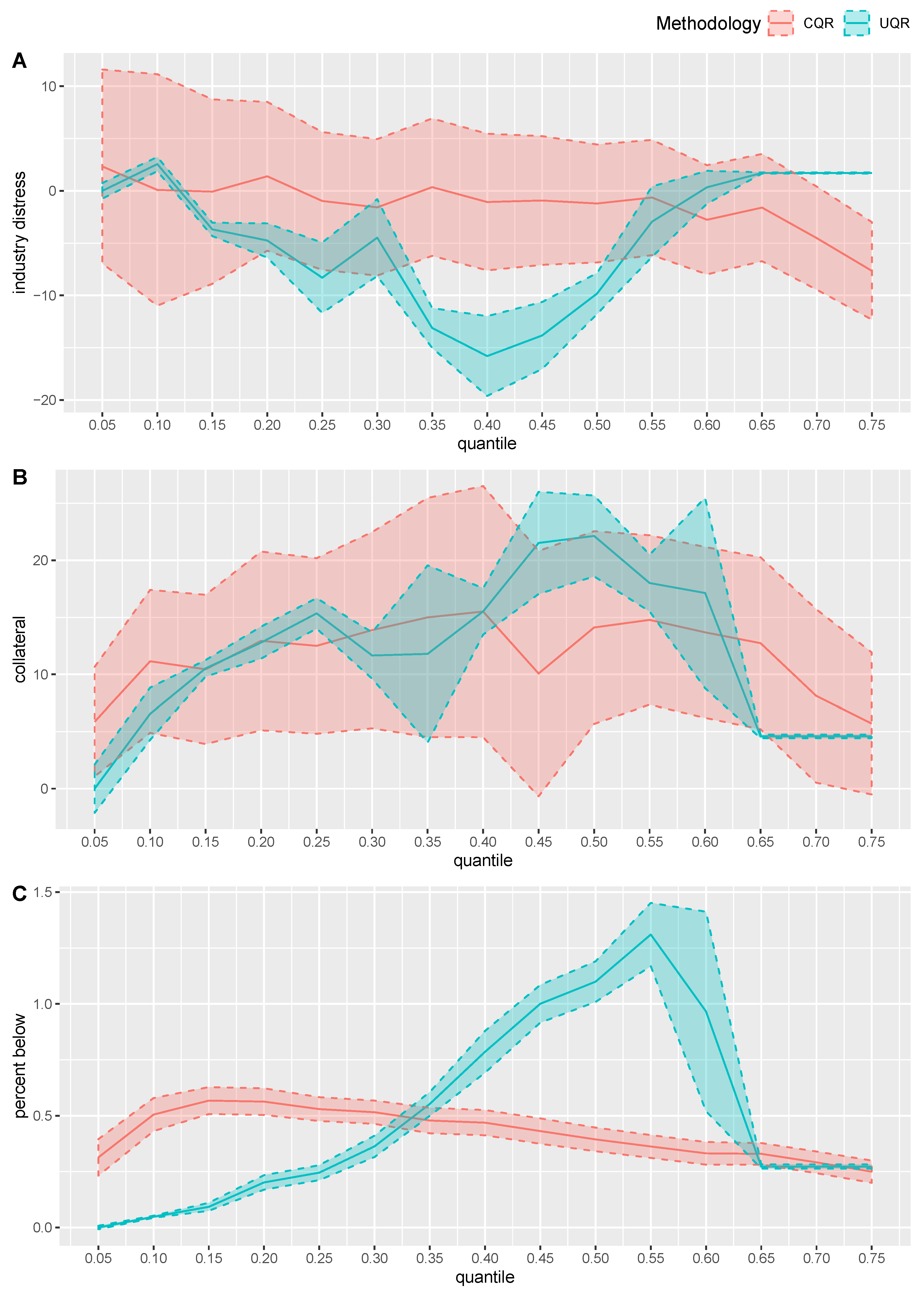
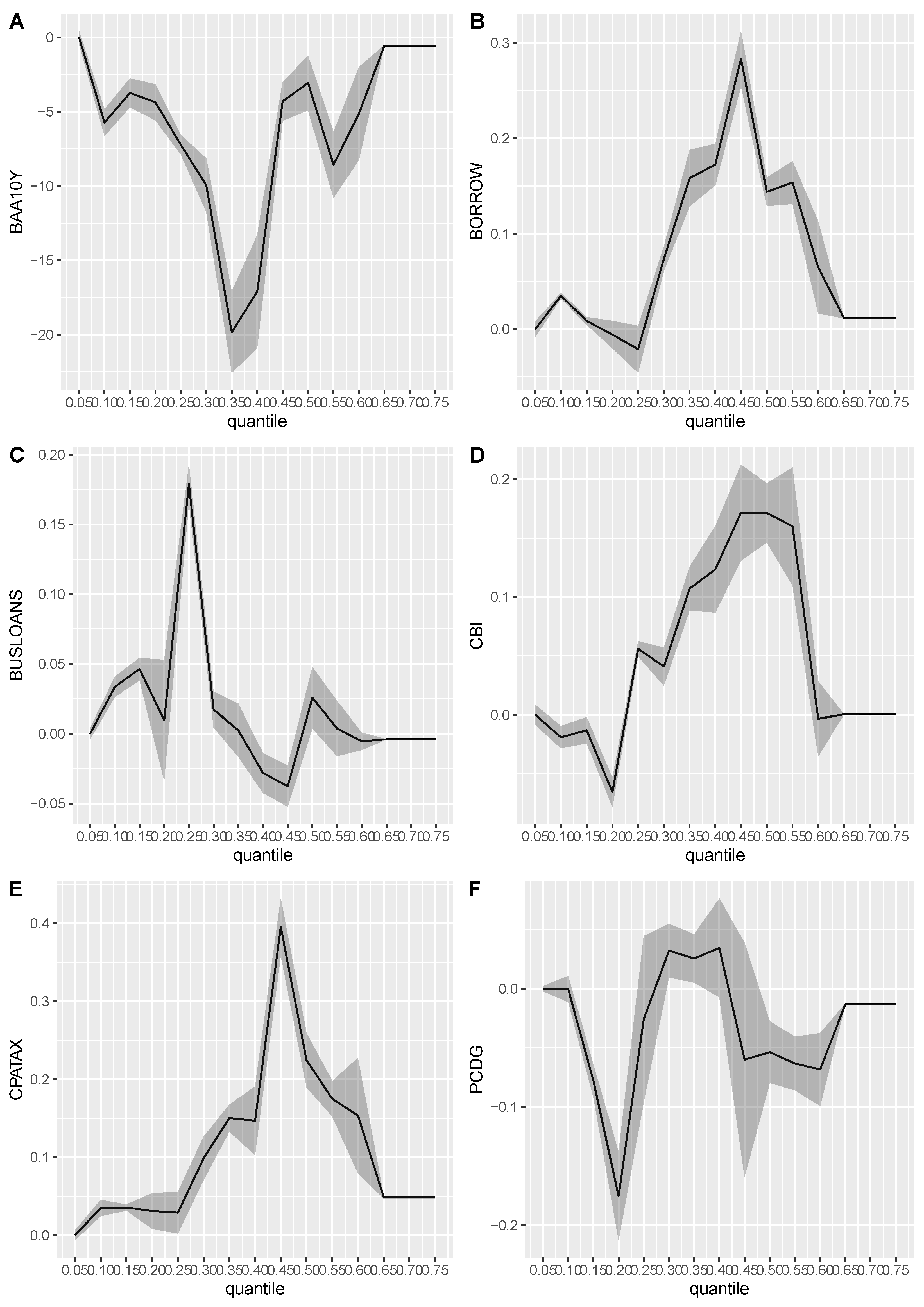
3.3. Unconditional Quantile Regression Estimates
4. Conclusions
Supplementary Materials
Author Contributions
Funding
Data Availability Statement
Acknowledgments
Conflicts of Interest
Abbreviations
| LGD | Loss given default |
| CQR | Conditional quantile regression |
| UQR | Unconditional quantile regression |
| DML | Double machine learning |
| Lasso | Least absolute shrinkage and selection operator |
| RIF | Recentered influence function |
| 1 | https://eba.europa.eu/regulation-and-policy/single-rulebook/ (accessed on 1 January 2019). |
| 2 | |
| 3 | |
| 4 | We implement the lasso selection by the rlasso function in the hdm packages of the R program; see Belloni et al. (2014a) for further information. |
| 5 | The term spread, 10-year treasury minus 3-month treasury rate used in Krüger and Rösch (2017) is also adopted in Nazemi and Fabozzi (2018). |
| 6 | Nazemi and Fabozzi (2018) identify 24 out of 179 macroeconomic variables when applying the lasso approach to the recovery rates of the S&P Capital IQ-similar corporate bond data in the years 2002–2012. |
| 7 | We use the bootstrapping method to estimate the standard errors of UQR and CQR coefficients. The bootstrap replication number is set to be 5000. The heteroskedasticity-robust standard errors are used in OLS coefficients. R packages uqr and quantreg estimate the coefficients and standard errors of UQR and CQR; lmtest calculates the heteroskedasticity-robust standard errors of OLS estimates. |
References
- Acharya, Viral V., Sreedhar T. Bharath, and Anand Srinivasan. 2007. Does industry-wide distress affect defaulted firms? Evidence from creditor recoveries. Journal of Financial Economics 85: 787–821. [Google Scholar] [CrossRef]
- Altman, Edward, Brooks Brady, Andrea Resti, and Andrea Sironi. 2005. The link between default and recovery rates: Theory, empirical evidence, and implications. The Journal of Business 78: 2203–28. [Google Scholar] [CrossRef]
- Bastos, João A. 2010. Forecasting bank loans loss-given-default. Journal of Banking & Finance 34: 2510–17. [Google Scholar]
- BCBS. 2004. International Convergence of Capital Measurement and Capital Standards: A Revised Framework. Basel: Basel Committee on Banking Supervision. [Google Scholar]
- BCBS. 2005. Guidance on Paragraph 468 of the Framework Document. Basel: Basel Committee on Banking Supervision. [Google Scholar]
- Belloni, Alexandre, Victor Chernozhukov, and Christian Hansen. 2014a. High-dimensional methods and inference on structural and treatment effects. Journal of Economic Perspectives 28: 29–50. [Google Scholar] [CrossRef]
- Belloni, Alexandre, Victor Chernozhukov, and Christian Hansen. 2014b. Inference on treatment effects after selection among high-dimensional controls. The Review of Economic Studies 81: 608–50. [Google Scholar] [CrossRef]
- Borah, Bijan J., and Anirban Basu. 2013. Highlighting differences between conditional and unconditional quantile regression approaches through an application to assess medication adherence. Health Economics 22: 1052–70. [Google Scholar] [CrossRef]
- Bruche, Max, and Carlos González-Aguado. 2010. Recovery rates, default probabilities, and the credit cycle. Journal of Banking & Finance 34: 754–64. [Google Scholar]
- Chang, Yuanchen, Yi-Ting Hsieh, Wenchien Liu, and Peter Miu. 2020. Intra-industry bankruptcy contagion: Evidence from the pricing of industry recovery rates. European Financial Management 26: 503–34. [Google Scholar] [CrossRef]
- Chava, Sudheer, Catalina Stefanescu, and Stuart Turnbull. 2011. Modeling the loss distribution. Management Science 57: 1267–87. [Google Scholar] [CrossRef]
- Chen, Jau-er, and Chen-Wei Hsiang. 2019. Causal random forests model using instrumental variable quantile regression. Econometrics 7: 49. [Google Scholar] [CrossRef]
- Chen, Jau-er, Chien-Hsun Huang, and Jia-Jyun Tien. 2021. Debiased/Double machine learning for instrumental variable quantile regressions. Econometrics 9: 15. [Google Scholar] [CrossRef]
- EBA. 2018. Final Draft Regulatory Technical Standards on the Specification of the Nature, Severity and Duration of an Economic Downturn in Accordance with Articles 181(3)(a) and 182(4)(a) of Regulation (EU) No 575/2013. London: European Banking Authority. [Google Scholar]
- EBA. 2019. Final Report: Guidelines for the Estimation of LGD Appropriate for an Economic Downturn. London: European Banking Authority. [Google Scholar]
- Feng, Guanhao, Stefano Giglio, and Dacheng Xiu. 2020. Taming the factor zoo: A test of new factors. The Journal of Finance 75: 1327–70. [Google Scholar] [CrossRef]
- Firpo, Sergio, Nicole M. Fortin, and Thomas Lemieux. 2009. Unconditional quantile regressions. Econometrica 77: 953–73. [Google Scholar]
- Gambetti, Paolo, Geneviève Gauthier, and Frédéric Vrins. 2019. Recovery rates: Uncertainty certainly matters. Journal of Banking & Finance 106: 371–83. [Google Scholar]
- Gürtler, Marc, and Martin Hibbeln. 2013. Improvements in loss given default forecasts for bank loans. Journal of Banking & Finance 37: 2354–66. [Google Scholar]
- Hartmann-Wendels, Thomas, Patrick Miller, and Eugen Töws. 2014. Loss given default for leasing: Parametric and nonparametric estimations. Journal of Banking & Finance 40: 364–75. [Google Scholar]
- Jankowitsch, Rainer, Florian Nagler, and Marti G. Subrahmanyam. 2014. The determinants of recovery rates in the US corporate bond market. Journal of Financial Economics 114: 155–77. [Google Scholar] [CrossRef]
- James, Christopher, and Atay Kizilaslan. 2014. Asset specificity, industry-driven recovery risk, and loan pricing. Journal of Financial and Quantitative Analysis 49: 599–631. [Google Scholar] [CrossRef]
- Kellner, Ralf, Maximilian Nagl, and Daniel Rösch. 2022. Opening the black box—Quantile neural networks for loss given default prediction. Journal of Banking & Finance 134: 106334. [Google Scholar]
- Koenker, Roger. 2005. Quantile Regression. Cambridge: Cambridge University Press. [Google Scholar]
- Koenker, Roger, and Gilbert Bassett. 1978. Regression quantiles. Econometrica 46: 33–50. [Google Scholar] [CrossRef]
- Krüger, Steffen, and Daniel Rösch. 2017. Downturn LGD modeling using quantile regression. Journal of Banking & Finance 79: 42–56. [Google Scholar]
- Nazemi, Abdolreza, and Frank J. Fabozzi. 2018. Macroeconomic variable selection for creditor recovery rates. Journal of Banking & Finance 89: 14–25. [Google Scholar]
- Nazemi, Abdolreza, Friedrich Baumann, and Frank J. Fabozzi. 2022. Intertemporal defaulted bond recoveries prediction via machine learning. European Journal of Operational Research 297: 1162–77. [Google Scholar] [CrossRef]
- Nazemi, Abdolreza, Konstantin Hdidenreich, and Frank J. Fabozzi. 2018. Improving corporate bond recovery rate prediction using multi-factor support vector regressions. European Journal of Operational Research 271: 664–75. [Google Scholar] [CrossRef]
- Maclean, Johanna Catherine, Douglas A. Webber, and Joachim Marti. 2014. An application of unconditional quantile regression to cigarette taxes. Journal of Policy Analysis and Management 33: 188–210. [Google Scholar] [CrossRef]
- Porter, Stephen R. 2015. Quantile regression: Analyzing changes in distributions instead of means. In Higher Education: Handbook of Theory and Research. New York: Springer. [Google Scholar]
- Qi, Min, and Xinlei Zhao. 2011. Comparison of modeling methods for loss given default. Journal of Banking & Finance 35: 2842–55. [Google Scholar]
- Sasaki, Yuya, Takuya Ura, and Yichong Zhang. 2022. Unconditional quantile regression with high-dimensional data. Quantitative Economics 13: 955–78. [Google Scholar] [CrossRef]
- Shleifer, Andrel, and Robert W. Vishny. 1992. Liquidation values and debt capacity: A market equilibrium approach. The Journal of Finance 47: 1343–66. [Google Scholar] [CrossRef]
- Siao, Jhao-Siang, Ruey-Ching Hwang, and Chih-Kang Chu. 2016. Predicting recovery rates using logistic quantile regression with bounded outcomes. Quantitative Finance 16: 777–92. [Google Scholar] [CrossRef]
- Silverman, Bernard W. 1986. Density Estimation for Statistics and Data Analysis. London: Chapman Hall/CRC Monographs. [Google Scholar]
- Somers, Mark, and Joe Whittaker. 2007. Quantile regression for modelling distributions of profit and loss. European Journal of Operational Research 183: 1477–87. [Google Scholar] [CrossRef]


| Variable | Definitions |
|---|---|
| collateral | A dummy variable equals one if the debt has collateral, and zero otherwise. |
| industry | Instrument’s issuer’s industry is classified by the 30 Fama–French industry portfolio classification. |
| industry distress | A dummy variable that equals one if the median stock returns of the firms with the same industry classification to the instrument’s issuer is less than −30% as Acharya et al. (2007). The year of the annual stock return is measured as the year at the middlepoint between default and emergence date of the instrument. |
| instrument type | Instrument type. One of Revolver, Term Loan, Senior Secured Bonds, Senior Subordinated Bonds, Senior Unsecured Bonds, Subordinated Bonds, Junior Subordinated Bonds. |
| percentage below | At the time of default, debt below is the total dollar amount outstanding of all defaulted debt that is contractually subordinate to the current instrument. Percentage below is debt below divided by the total issuer’s debt. |
| rank | Collateral quality rank. Moody’s DRD database ranks instrument’s collateral quality as 1, 2, ⋯, 8. We define the rank as 1, 2, 3, 4 by winsorizing the original rank at 4 due to the limited observations with ranking above 4. |
| recovery rate | Moody’s recommended recovery rate. Moody’s Investor Service (MIS), based on internal research standards, recommend the recovery rate based on either trading price, liquidity, or settlement discounted recovery. |
| year | Instrument’s year dummy is created as the year at the middlepoint between default and emergence date of the instrument. |
| Year | 10% | 25% | 50% | 75% | Avg. | Obs. | Freq. |
|---|---|---|---|---|---|---|---|
| Recovery Rate | 1.93 | 20.61 | 65.41 | 100.00 | 59.41 | 5334 | 100.00 |
| 1990 | 6.23 | 18.78 | 51.76 | 100.00 | 54.56 | 94 | 1.76 |
| 1991 | 1.90 | 16.00 | 71.20 | 100.00 | 59.66 | 175 | 3.28 |
| 1992 | 2.25 | 16.05 | 38.60 | 83.44 | 48.91 | 258 | 4.84 |
| 1993 | 2.51 | 23.42 | 94.56 | 100.00 | 66.24 | 161 | 3.02 |
| 1994 | 0.95 | 24.10 | 69.13 | 100.00 | 60.52 | 140 | 2.62 |
| 1995 | 0.15 | 30.64 | 76.47 | 100.00 | 64.23 | 34 | 0.64 |
| 1996 | 8.89 | 29.55 | 62.64 | 100.00 | 63.22 | 108 | 2.02 |
| 1997 | 6.26 | 16.18 | 79.85 | 100.00 | 63.97 | 65 | 1.22 |
| 1998 | 6.34 | 21.81 | 49.92 | 100.00 | 57.46 | 64 | 1.20 |
| 1999 | 5.19 | 20.70 | 61.44 | 100.00 | 59.88 | 141 | 2.64 |
| 2000 | 0.75 | 14.11 | 60.48 | 100.00 | 55.97 | 173 | 3.24 |
| 2001 | 0.47 | 7.48 | 46.86 | 100.00 | 51.23 | 352 | 6.60 |
| 2002 | 1.60 | 15.27 | 36.71 | 100.00 | 50.87 | 786 | 14.74 |
| 2003 | 1.32 | 21.83 | 49.82 | 100.00 | 53.09 | 562 | 10.54 |
| 2004 | 15.85 | 52.48 | 73.85 | 100.00 | 70.07 | 402 | 7.52 |
| 2005 | 24.82 | 66.12 | 100.00 | 100.00 | 79.23 | 114 | 2.14 |
| 2006 | 17.64 | 53.31 | 88.72 | 100.00 | 74.63 | 162 | 3.04 |
| 2007 | 3.67 | 56.64 | 96.77 | 100.00 | 76.97 | 114 | 2.14 |
| 2008 | 8.49 | 37.53 | 100.00 | 100.00 | 68.01 | 171 | 3.21 |
| 2009 | 1.15 | 21.06 | 76.44 | 100.00 | 62.60 | 516 | 9.67 |
| 2010 | 1.56 | 29.26 | 73.36 | 100.00 | 63.49 | 180 | 3.37 |
| 2011 | 0.00 | 0.44 | 58.57 | 100.00 | 53.19 | 55 | 1.03 |
| 2012 | 4.25 | 42.91 | 100.00 | 100.00 | 71.72 | 147 | 2.76 |
| 2013 | 1.37 | 39.58 | 73.88 | 100.00 | 63.50 | 54 | 1.01 |
| 2014 | 0.42 | 26.18 | 73.72 | 100.00 | 60.83 | 35 | 0.66 |
| 2015 | 11.06 | 24.53 | 54.26 | 100.00 | 60.01 | 145 | 2.72 |
| 2016 | 0.63 | 7.05 | 24.18 | 92.33 | 41.98 | 122 | 2.29 |
| 2017 | 71.36 | 71.64 | 97.62 | 100.00 | 88.09 | 5 | 0.09 |
| Quantile | 10% | 25% | 50% | 75% | 90% | Avg. | Obs. |
|---|---|---|---|---|---|---|---|
| Recovery Rate | 1.93 | 20.61 | 65.41 | 100.00 | 100.00 | 59.41 | 5334 |
| Panel A: Collateral status | |||||||
| No | 0.00 | 5.10 | 29.01 | 74.27 | 100.00 | 41.00 | 2582 |
| Yes | 20.88 | 53.26 | 100.00 | 100.00 | 100.00 | 76.67 | 2752 |
| Panel B: Collateral quality rank | |||||||
| 1 | 24.14 | 58.17 | 100.00 | 100.00 | 100.00 | 78.07 | 2551 |
| 2 | 0.93 | 14.19 | 37.85 | 88.49 | 100.00 | 47.45 | 1791 |
| 3 | 0.00 | 1.44 | 18.10 | 60.73 | 100.00 | 34.05 | 659 |
| 4 | 0.00 | 0.82 | 16.31 | 64.20 | 98.52 | 30.89 | 333 |
| Panel C: Instrument type | |||||||
| Junior Subordinated | 0.00 | 0.00 | 3.35 | 21.60 | 88.88 | 20.49 | 73 |
| Revolver | 40.00 | 80.72 | 100.00 | 100.00 | 100.00 | 86.29 | 1112 |
| Senior Secured | 18.44 | 23.72 | 62.24 | 100.00 | 100.00 | 61.95 | 706 |
| Senior Subordinated | 0.00 | 1.36 | 14.96 | 49.72 | 82.09 | 28.37 | 508 |
| Senior Unsecured | 1.22 | 12.52 | 39.71 | 88.92 | 100.00 | 47.86 | 1528 |
| Subordinated | 0.00 | 0.10 | 14.67 | 48.60 | 98.06 | 28.55 | 365 |
| Term Loan | 16.52 | 47.09 | 100.00 | 100.00 | 100.00 | 74.58 | 1042 |
| Panel D: Industry distress | |||||||
| No | 1.96 | 20.91 | 66.87 | 100.00 | 100.00 | 60.22 | 4527 |
| Yes | 2.12 | 12.99 | 58.38 | 100.00 | 100.00 | 54.83 | 807 |
| Panel E: Instrument type × Industry distress | |||||||
| Junior Subordinated × Distress (No) | 0.00 | 0.00 | 3.31 | 21.73 | 90.75 | 21.24 | 70 |
| Junior Subordinated × Distress (Yes) | 0.87 | 2.18 | 4.35 | 4.40 | 4.43 | 2.93 | 3 |
| Revolver × Distress (No) | 42.08 | 80.99 | 100.00 | 100.00 | 100.00 | 86.65 | 949 |
| Revolver × Distress (Yes) | 29.35 | 78.42 | 100.00 | 100.00 | 100.00 | 84.23 | 163 |
| Senior Secured × Distress (No) | 18.78 | 24.07 | 63.31 | 100.00 | 100.00 | 62.52 | 655 |
| Senior Secured × Distress (Yes) | 12.78 | 18.64 | 50.42 | 99.13 | 100.00 | 54.67 | 51 |
| Senior Subordinated × Distress (No) | 0.00 | 1.61 | 14.85 | 48.62 | 80.27 | 28.07 | 446 |
| Senior Subordinated × Distress (Yes) | 0.03 | 0.75 | 15.63 | 54.54 | 92.55 | 30.57 | 62 |
| Senior Unsecured × Distress (No) | 1.41 | 15.32 | 47.29 | 100.00 | 100.00 | 51.45 | 1231 |
| Senior Unsecured × Distress (Yes) | 0.43 | 8.26 | 24.36 | 61.69 | 77.92 | 32.98 | 297 |
| Subordinated × Distress (No) | 0.00 | 0.11 | 14.85 | 45.04 | 88.47 | 27.33 | 323 |
| Subordinated × Distress (Yes) | 0.00 | 0.00 | 8.26 | 80.35 | 100.00 | 37.97 | 42 |
| Term Loan × Distress (No) | 17.78 | 46.93 | 100.00 | 100.00 | 100.00 | 74.18 | 853 |
| Term Loan × Distress (Yes) | 16.33 | 48.64 | 100.00 | 100.00 | 100.00 | 76.38 | 189 |
| Percentile | 5% | 10% | 15% | 20% | 25% | 30% | 35% | 40% | 45% | 50% | 55% | 60% | 65% | 70% | 75% |
|---|---|---|---|---|---|---|---|---|---|---|---|---|---|---|---|
| BAA10Y | 1 | 1 | 1 | 1 | 1 | 1 | 1 | 1 | 1 | 1 | 1 | 1 | 1 | 1 | 1 |
| BORROW | 1 | 1 | 1 | 1 | 1 | 1 | 1 | 1 | 1 | 1 | 1 | 1 | 1 | 1 | 1 |
| BUSLOANS | 1 | 1 | 1 | 1 | 1 | 1 | 1 | 1 | 1 | 1 | 1 | 1 | 1 | 1 | 1 |
| CBI | 1 | 1 | 1 | 1 | 1 | 1 | 1 | 1 | 1 | 1 | 1 | 1 | 1 | 1 | 1 |
| CPATAX | 1 | 1 | 1 | 1 | 1 | 1 | 1 | 1 | 1 | 1 | 1 | 1 | 1 | 1 | 1 |
| debt_ebitda | 1 | 1 | 1 | 1 | 1 | 1 | 1 | 1 | 1 | 1 | 1 | 1 | 1 | 1 | 1 |
| fcf_ocf | 1 | 1 | 1 | 1 | 1 | 1 | 1 | 1 | 1 | 1 | 1 | 1 | 1 | 1 | 1 |
| industry return | 1 | 1 | 1 | 1 | 1 | 1 | 1 | 1 | 1 | 1 | 1 | 1 | 1 | 1 | 1 |
| industry volatility | 1 | 1 | 1 | 1 | 1 | 1 | 1 | 1 | 1 | 1 | 1 | 1 | 1 | 1 | 1 |
| opmad | 1 | 1 | 1 | 1 | 1 | 1 | 1 | 1 | 1 | 1 | 1 | 1 | 1 | 1 | 1 |
| PCDG | 1 | 1 | 1 | 1 | 1 | 1 | 1 | 1 | 1 | 1 | 1 | 1 | 1 | 1 | 1 |
| S&P500 | 1 | 1 | 1 | 1 | 1 | 1 | 1 | 1 | 1 | 1 | 1 | 1 | 1 | 1 | 1 |
| cash_ratio | 0 | 1 | 0 | 0 | 0 | 0 | 0 | 0 | 0 | 0 | 0 | 0 | 0 | 0 | 0 |
| ps | 0 | 1 | 1 | 1 | 1 | 1 | 1 | 1 | 1 | 1 | 1 | 1 | 1 | 1 | 1 |
| quick_ratio | 0 | 1 | 1 | 0 | 0 | 0 | 0 | 0 | 0 | 0 | 0 | 0 | 0 | 0 | 0 |
| GProf | 0 | 1 | 0 | 0 | 0 | 0 | 0 | 0 | 0 | 0 | 0 | 0 | 0 | 0 | 0 |
| CAPEI | 0 | 0 | 1 | 0 | 1 | 0 | 0 | 0 | 0 | 0 | 0 | 0 | 0 | 0 | 0 |
| staff_sale | 0 | 0 | 1 | 1 | 1 | 1 | 1 | 1 | 0 | 0 | 0 | 0 | 0 | 0 | 0 |
| lt_debt | 0 | 0 | 1 | 0 | 0 | 0 | 0 | 1 | 1 | 1 | 1 | 1 | 0 | 0 | 0 |
| TEDRATE | 0 | 0 | 1 | 0 | 1 | 0 | 0 | 0 | 0 | 0 | 0 | 0 | 1 | 1 | 1 |
| CES3000000008 | 0 | 0 | 1 | 1 | 1 | 0 | 0 | 0 | 0 | 0 | 0 | 0 | 0 | 0 | 0 |
| DPIC96 | 0 | 0 | 1 | 1 | 0 | 0 | 0 | 0 | 0 | 0 | 0 | 0 | 0 | 0 | 0 |
| npm | 0 | 0 | 1 | 0 | 0 | 0 | 0 | 0 | 0 | 0 | 0 | 0 | 0 | 0 | 0 |
| M2SL | 0 | 0 | 0 | 1 | 1 | 0 | 0 | 0 | 0 | 0 | 0 | 0 | 0 | 0 | 0 |
| TOTALSL | 0 | 0 | 0 | 1 | 0 | 0 | 0 | 0 | 0 | 0 | 0 | 0 | 0 | 0 | 0 |
| M1SL | 0 | 0 | 0 | 1 | 1 | 1 | 1 | 0 | 1 | 1 | 1 | 0 | 0 | 0 | 0 |
| EMRATIO | 0 | 0 | 0 | 0 | 1 | 0 | 0 | 0 | 0 | 0 | 0 | 0 | 0 | 0 | 0 |
| VIXCLS | 0 | 0 | 0 | 0 | 1 | 1 | 1 | 0 | 0 | 0 | 0 | 0 | 0 | 0 | 0 |
| IPFINAL | 0 | 0 | 0 | 0 | 1 | 0 | 1 | 0 | 0 | 0 | 0 | 0 | 0 | 0 | 0 |
| PEG_1yrforward | 0 | 0 | 0 | 0 | 0 | 1 | 1 | 0 | 0 | 0 | 1 | 1 | 1 | 1 | 1 |
| UEMP5TO14 | 0 | 0 | 0 | 0 | 0 | 1 | 1 | 0 | 0 | 0 | 0 | 0 | 0 | 0 | 0 |
| PERMITW | 0 | 0 | 0 | 0 | 0 | 1 | 1 | 1 | 0 | 0 | 0 | 0 | 0 | 0 | 0 |
| MORTG | 0 | 0 | 0 | 0 | 0 | 1 | 0 | 0 | 0 | 0 | 0 | 0 | 0 | 0 | 0 |
| dpr | 0 | 0 | 0 | 0 | 0 | 0 | 1 | 1 | 0 | 0 | 0 | 0 | 0 | 0 | 0 |
| CNCF | 0 | 0 | 0 | 0 | 0 | 0 | 0 | 0 | 1 | 0 | 0 | 0 | 0 | 0 | 0 |
| IPB51200SQ | 0 | 0 | 0 | 0 | 0 | 0 | 0 | 0 | 1 | 1 | 0 | 0 | 0 | 0 | 0 |
| curr_ratio | 0 | 0 | 0 | 0 | 0 | 0 | 0 | 0 | 0 | 0 | 1 | 1 | 1 | 1 | 1 |
| HSN1F | 0 | 0 | 0 | 0 | 0 | 0 | 0 | 0 | 0 | 0 | 1 | 1 | 1 | 1 | 1 |
| USROE | 0 | 0 | 0 | 0 | 0 | 0 | 0 | 0 | 0 | 0 | 0 | 1 | 1 | 1 | 1 |
| debt_at | 0 | 0 | 0 | 0 | 0 | 0 | 0 | 0 | 0 | 0 | 0 | 0 | 1 | 1 | 1 |
| totdebt_invcap | 0 | 0 | 0 | 0 | 0 | 0 | 0 | 0 | 0 | 0 | 0 | 0 | 1 | 1 | 1 |
| HOUSTNE | 0 | 0 | 0 | 0 | 0 | 0 | 0 | 0 | 0 | 0 | 0 | 0 | 1 | 1 | 1 |
| covariates no. | 12 | 16 | 21 | 19 | 22 | 20 | 21 | 17 | 17 | 16 | 18 | 18 | 21 | 21 | 21 |
| UQR | CQR | OLS | |||||||
|---|---|---|---|---|---|---|---|---|---|
| Coef. | s.e. | p-Value | Coef. | s.e. | p-Value | Coef. | s.e. | p-Value | |
| constant | 565.02 | 31.86 | 0.00 | 119.12 | 76.87 | 0.12 | 198.88 | 59.09 | 0.00 |
| industry distress | −9.82 | 1.00 | 0.00 | −1.21 | 2.88 | 0.67 | −3.56 | 2.91 | 0.22 |
| percent below | 1.10 | 0.05 | 0.00 | 0.39 | 0.03 | 0.00 | 0.41 | 0.02 | 0.00 |
| collateral | 22.14 | 1.81 | 0.00 | 14.11 | 4.31 | 0.00 | 9.33 | 2.22 | 0.00 |
| Junior Subordinated | −30.66 | 3.85 | 0.00 | −26.19 | 4.76 | 0.00 | −20.09 | 4.19 | 0.00 |
| Senior Secured | −37.24 | 1.53 | 0.00 | −12.06 | 2.59 | 0.00 | −12.43 | 1.69 | 0.00 |
| Senior Subordinated | −35.85 | 2.45 | 0.00 | −26.38 | 4.45 | 0.00 | −18.51 | 2.65 | 0.00 |
| Senior Unsecured | −9.07 | 1.81 | 0.00 | −2.98 | 4.18 | 0.48 | −2.24 | 2.37 | 0.34 |
| Subordinated | −31.00 | 3.19 | 0.00 | −23.13 | 4.92 | 0.00 | −16.43 | 2.80 | 0.00 |
| Term Loan | −13.44 | 0.67 | 0.00 | −1.48 | 1.49 | 0.32 | −6.08 | 1.38 | 0.00 |
| Junior Subordinated × distress | −22.31 | 2.22 | 0.00 | −14.80 | 10.33 | 0.15 | −15.58 | 17.03 | 0.36 |
| Senior Secured × distress | −5.63 | 3.49 | 0.11 | −1.42 | 9.79 | 0.89 | −3.52 | 4.89 | 0.47 |
| Senior Subordinated × distress | 13.58 | 1.01 | 0.00 | 1.39 | 4.80 | 0.77 | 6.35 | 4.60 | 0.17 |
| Senior Unsecured × distress | −10.27 | 1.26 | 0.00 | −5.14 | 4.10 | 0.21 | −7.04 | 3.16 | 0.03 |
| Subordinated × distress | 56.38 | 6.13 | 0.00 | 5.93 | 9.06 | 0.51 | 19.45 | 5.33 | 0.00 |
| Term Loan × distress | 7.37 | 1.12 | 0.00 | 4.36 | 3.30 | 0.19 | 4.61 | 3.34 | 0.17 |
| BAA10Y | −3.07 | 0.94 | 0.00 | −6.10 | 2.18 | 0.01 | −3.49 | 1.80 | 0.05 |
| BORROW | 0.14 | 0.01 | 0.00 | 0.06 | 0.02 | 0.00 | 0.06 | 0.02 | 0.00 |
| BUSLOANS | 0.03 | 0.01 | 0.02 | 0.02 | 0.02 | 0.42 | 0.01 | 0.01 | 0.61 |
| CBI | 0.17 | 0.01 | 0.00 | 0.00 | 0.03 | 0.94 | 0.03 | 0.02 | 0.20 |
| CPATAX | 0.22 | 0.02 | 0.00 | 0.08 | 0.02 | 0.00 | 0.08 | 0.02 | 0.00 |
| IPB51200SQ | −4.52 | 0.37 | 0.00 | −0.42 | 0.81 | 0.60 | −1.04 | 0.67 | 0.12 |
| M1SL | 0.00 | 0.01 | 0.76 | 0.03 | 0.02 | 0.26 | 0.02 | 0.02 | 0.22 |
| PCDG | −0.05 | 0.01 | 0.00 | −0.01 | 0.04 | 0.83 | −0.04 | 0.03 | 0.16 |
| S&P 500 return | 11.75 | 3.07 | 0.00 | 11.38 | 4.99 | 0.02 | 8.28 | 3.32 | 0.01 |
| ps | −18.84 | 1.07 | 0.00 | −8.13 | 1.60 | 0.00 | −9.54 | 1.14 | 0.00 |
| opmad | −158.63 | 8.94 | 0.00 | −19.14 | 20.70 | 0.36 | −61.72 | 14.46 | 0.00 |
| fcf_ocf | −11.82 | 1.62 | 0.00 | 2.92 | 5.07 | 0.56 | −0.42 | 3.67 | 0.91 |
| debt_ebitda | 10.51 | 0.73 | 0.00 | 1.95 | 1.10 | 0.08 | 3.04 | 0.94 | 0.00 |
| lt_debt | −230.43 | 9.81 | 0.00 | −67.74 | 14.66 | 0.00 | −86.10 | 10.53 | 0.00 |
| industry return | 6.08 | 3.45 | 0.08 | −3.75 | 3.82 | 0.33 | 0.23 | 2.99 | 0.94 |
| industry volatility | −50.54 | 3.31 | 0.00 | −4.60 | 11.08 | 0.68 | −27.94 | 7.85 | 0.00 |
| rank dummy | yes | yes | yes | ||||||
| year dummy | yes | yes | yes | ||||||
| industry dummy | yes | yes | yes | ||||||
| UQR | CQR | |||||
|---|---|---|---|---|---|---|
| Quantile | Coef. | s.e. | p-Value | Coef. | s.e. | p-Value |
| 5% | 0.000 | 0.381 | 1.000 | 2.330 | 4.730 | 0.622 |
| 10% | 2.556 *** | 0.346 | 0.000 | 0.088 | 5.645 | 0.988 |
| 15% | -3.683 *** | 0.326 | 0.000 | −0.076 | 4.497 | 0.987 |
| 20% | -4.747 *** | 0.832 | 0.000 | 1.392 | 3.629 | 0.701 |
| 25% | -8.307 *** | 1.714 | 0.000 | −0.968 | 3.360 | 0.773 |
| 30% | -4.475 ** | 1.878 | 0.017 | −1.580 | 3.328 | 0.635 |
| 35% | -13.112 *** | 0.970 | 0.000 | 0.353 | 3.351 | 0.916 |
| 40% | -15.798 *** | 1.945 | 0.000 | −1.069 | 3.333 | 0.748 |
| 45% | -13.829 *** | 1.632 | 0.000 | −0.923 | 3.140 | 0.769 |
| 50% | -9.817 *** | 1.000 | 0.000 | −1.210 | 2.877 | 0.674 |
| 55% | -2.943 * | 1.716 | 0.086 | −0.638 | 2.810 | 0.820 |
| 60% | 0.342 | 0.802 | 0.670 | −2.768 | 2.662 | 0.298 |
| 65% | 1.709 *** | 0.029 | 0.000 | −1.600 | 2.614 | 0.541 |
| 70% | 1.709 *** | 0.029 | 0.000 | −4.532 * | 2.513 | 0.071 |
| 75% | 1.709 *** | 0.029 | 0.000 | −7.657 *** | 2.378 | 0.001 |
| Percentile | 10% | 20% | 30% | 40% | 50% | 60% | 70% | |||||||
|---|---|---|---|---|---|---|---|---|---|---|---|---|---|---|
| Coef. | s.e. | Coef. | s.e. | Coef. | s.e. | Coef. | s.e. | Coef. | s.e. | Coef. | s.e. | Coef. | s.e. | |
| industry distress | 2.56 | 0.35 | −4.75 | 0.83 | −4.48 | 1.88 | −15.80 | 1.95 | −9.82 | 1.00 | 0.34 | 0.80 | 1.71 | 0.03 |
| percent below | 0.05 | 0.00 | 0.20 | 0.02 | 0.36 | 0.02 | 0.79 | 0.05 | 1.10 | 0.05 | 0.97 | 0.23 | 0.27 | 0.00 |
| collateral | 6.56 | 1.16 | 12.79 | 0.72 | 11.66 | 1.04 | 15.52 | 1.04 | 22.14 | 1.81 | 17.14 | 4.26 | 4.58 | 0.08 |
| Junior Subordinated | −18.69 | 1.25 | −29.95 | 2.38 | −40.35 | 1.39 | −42.10 | 2.15 | −30.66 | 3.85 | −14.30 | 2.04 | −4.82 | 0.08 |
| Senior Secured | 2.16 | 0.26 | −1.59 | 1.10 | −13.59 | 0.65 | −21.15 | 1.08 | −37.24 | 1.53 | −34.29 | 6.50 | −10.37 | 0.18 |
| Senior Subordinated | −6.62 | 0.46 | −22.63 | 2.26 | −30.41 | 1.96 | −35.22 | 1.75 | −35.85 | 2.45 | −25.67 | 5.02 | −8.02 | 0.14 |
| Senior Unsecured | 6.86 | 0.72 | 5.20 | 2.28 | 0.13 | 0.61 | −1.00 | 0.99 | −9.07 | 1.81 | −6.28 | 0.61 | −3.15 | 0.05 |
| Subordinated | −11.58 | 0.70 | −21.14 | 3.54 | −31.15 | 1.37 | −31.86 | 1.75 | −31.00 | 3.19 | −14.55 | 2.47 | −4.76 | 0.08 |
| Term Loan | −1.15 | 0.33 | −4.64 | 0.53 | −4.84 | 0.64 | −10.82 | 0.58 | −13.44 | 0.67 | −14.47 | 3.28 | −4.12 | 0.07 |
| Junior Subordinated × distress | 5.42 | 1.68 | −46.22 | 2.08 | −35.79 | 2.51 | −40.19 | 2.02 | −22.31 | 2.22 | −3.99 | 1.24 | −1.75 | 0.03 |
| Senior Secured × distress | 4.21 | 0.57 | 3.23 | 0.89 | −3.05 | 1.46 | 0.80 | 1.57 | −5.63 | 3.49 | −10.65 | 3.88 | −2.90 | 0.05 |
| Senior Subordinated × distress | −7.67 | 0.72 | 5.64 | 0.87 | 11.16 | 2.14 | 12.57 | 2.18 | 13.58 | 1.01 | 9.90 | 2.52 | 0.48 | 0.01 |
| Senior Unsecured × distress | −0.19 | 0.36 | −9.70 | 1.21 | −9.34 | 1.99 | −12.61 | 0.88 | −10.27 | 1.26 | −18.22 | 2.86 | −5.54 | 0.09 |
| Subordinated × distress | 2.97 | 0.66 | 5.30 | 1.45 | 26.77 | 2.77 | 53.36 | 3.13 | 56.38 | 6.13 | 22.05 | 9.50 | 2.87 | 0.05 |
| Term Loan × distress | 1.95 | 0.45 | 6.15 | 0.71 | 0.48 | 1.72 | 13.31 | 1.53 | 7.37 | 1.12 | 4.52 | 1.47 | 1.08 | 0.02 |
| BAA10Y | −5.73 | 0.46 | −4.36 | 0.62 | −9.93 | 0.92 | −17.11 | 1.94 | −3.07 | 0.94 | −5.12 | 1.59 | −0.55 | 0.01 |
| BORROW | 0.04 | 0.00 | −0.01 | 0.01 | 0.07 | 0.01 | 0.17 | 0.01 | 0.14 | 0.01 | 0.06 | 0.02 | 0.01 | 0.00 |
| BUSLOANS | 0.03 | 0.00 | 0.01 | 0.02 | 0.02 | 0.01 | −0.03 | 0.01 | 0.03 | 0.01 | −0.01 | 0.00 | 0.00 | 0.00 |
| CBI | −0.02 | 0.00 | −0.07 | 0.01 | 0.04 | 0.01 | 0.12 | 0.02 | 0.17 | 0.01 | 0.00 | 0.02 | 0.00 | 0.00 |
| CPATAX | 0.03 | 0.01 | 0.03 | 0.01 | 0.10 | 0.01 | 0.15 | 0.02 | 0.22 | 0.02 | 0.15 | 0.04 | 0.05 | 0.00 |
| PCDG | 0.00 | 0.01 | −0.18 | 0.02 | 0.03 | 0.01 | 0.03 | 0.02 | −0.05 | 0.01 | −0.07 | 0.02 | −0.01 | 0.00 |
| S&P 500 return | 2.03 | 0.37 | 3.90 | 0.53 | 6.66 | 1.76 | 42.03 | 1.91 | 11.75 | 3.07 | −3.13 | 1.21 | 0.15 | 0.00 |
| opmad | −26.50 | 2.51 | −16.56 | 8.12 | −88.03 | 7.62 | −78.88 | 15.05 | −158.63 | 8.94 | −141.31 | 37.84 | −28.51 | 0.49 |
| fcf_ocf | 1.27 | 0.44 | 10.20 | 0.78 | 3.20 | 1.68 | −3.16 | 0.79 | −11.82 | 1.62 | 4.61 | 1.13 | 0.51 | 0.01 |
| debt_ebitda | 1.55 | 0.23 | 1.09 | 0.31 | 2.40 | 0.42 | 2.38 | 0.41 | 10.51 | 0.73 | 3.04 | 1.15 | 1.66 | 0.03 |
| ps | −4.76 | 0.20 | −9.32 | 0.68 | −14.08 | 1.56 | −20.87 | 0.94 | −18.84 | 1.07 | −9.25 | 2.61 | −2.56 | 0.04 |
| industry return | 0.62 | 0.71 | −1.96 | 1.99 | −14.55 | 0.99 | −7.88 | 2.02 | 6.08 | 3.45 | −5.33 | 1.29 | 1.71 | 0.03 |
| industry volatility | −4.94 | 0.93 | −24.63 | 6.26 | −34.45 | 2.26 | −41.34 | 3.29 | −50.54 | 3.31 | −47.96 | 11.02 | −8.63 | 0.15 |
| rank | yes | yes | yes | yes | yes | yes | yes | |||||||
| year | yes | yes | yes | yes | yes | yes | yes | |||||||
| industry | yes | yes | yes | yes | yes | yes | yes | |||||||
| Percentile | 10% | 20% | 30% | 40% | 50% | 60% | 70% | |||||||
|---|---|---|---|---|---|---|---|---|---|---|---|---|---|---|
| Coef. | s.e. | Coef. | s.e. | Coef. | s.e. | Coef. | s.e. | Coef. | s.e. | Coef. | s.e. | Coef. | s.e. | |
| CES3000000008 | 5.92 | 1.33 | ||||||||||||
| DPIC96 | 0.02 | 0.00 | ||||||||||||
| HOUSTNE | −0.04 | 0.00 | ||||||||||||
| HSN1F | −0.07 | 0.01 | −0.02 | 0.00 | ||||||||||
| IPB51200SQ | −4.52 | 0.37 | ||||||||||||
| M1SL | 0.11 | 0.01 | 0.08 | 0.01 | 0.00 | 0.01 | ||||||||
| M2SL | −0.03 | 0.01 | ||||||||||||
| MORTG | 11.13 | 1.35 | ||||||||||||
| PERMITW | −0.07 | 0.01 | −0.17 | 0.01 | ||||||||||
| TEDRATE | 5.43 | 0.09 | ||||||||||||
| TOTALSL | 0.13 | 0.02 | ||||||||||||
| UEMP5TO14 | 0.02 | 0.00 | ||||||||||||
| USROE | −4.38 | 1.01 | −1.24 | 0.02 | ||||||||||
| VIXCLS | −0.61 | 0.03 | ||||||||||||
| cash_ratio | −0.08 | 1.67 | ||||||||||||
| curr_ratio | −30.00 | 7.16 | −14.90 | 0.25 | ||||||||||
| debt_at | −22.42 | 0.38 | ||||||||||||
| dpr | 60.47 | 3.40 | ||||||||||||
| GProf | 52.56 | 3.82 | ||||||||||||
| lt_debt | −147.04 | 11.76 | −230.43 | 9.81 | −146.79 | 41.71 | ||||||||
| PEG_1yrforward | 20.09 | 2.29 | 21.02 | 5.20 | 4.77 | 0.08 | ||||||||
| quick_ratio | −3.75 | 0.79 | ||||||||||||
| staff_sale | 223.44 | 9.14 | 162.07 | 13.56 | 243.80 | 11.89 | ||||||||
| totdebt_invcap | −47.02 | 0.80 | ||||||||||||
Disclaimer/Publisher’s Note: The statements, opinions and data contained in all publications are solely those of the individual author(s) and contributor(s) and not of MDPI and/or the editor(s). MDPI and/or the editor(s) disclaim responsibility for any injury to people or property resulting from any ideas, methods, instructions or products referred to in the content. |
© 2023 by the authors. Licensee MDPI, Basel, Switzerland. This article is an open access article distributed under the terms and conditions of the Creative Commons Attribution (CC BY) license (https://creativecommons.org/licenses/by/4.0/).
Share and Cite
Chuang, H.-C.; Chen, J.-e. Exploring Industry-Distress Effects on Loan Recovery: A Double Machine Learning Approach for Quantiles. Econometrics 2023, 11, 6. https://doi.org/10.3390/econometrics11010006
Chuang H-C, Chen J-e. Exploring Industry-Distress Effects on Loan Recovery: A Double Machine Learning Approach for Quantiles. Econometrics. 2023; 11(1):6. https://doi.org/10.3390/econometrics11010006
Chicago/Turabian StyleChuang, Hui-Ching, and Jau-er Chen. 2023. "Exploring Industry-Distress Effects on Loan Recovery: A Double Machine Learning Approach for Quantiles" Econometrics 11, no. 1: 6. https://doi.org/10.3390/econometrics11010006
APA StyleChuang, H.-C., & Chen, J.-e. (2023). Exploring Industry-Distress Effects on Loan Recovery: A Double Machine Learning Approach for Quantiles. Econometrics, 11(1), 6. https://doi.org/10.3390/econometrics11010006