
Common Correlated Effects Estimation for Dynamic Heterogeneous Panels with Non-Stationary Multi-Factor Error Structures

Abstract
:1. Introduction
2. Dynamic Panel Data Model with Non-Stationary Unobserved Common Factors
2.1. The Model
2.2. CCE Estimation
3. Asymptotics of CCE Estimators with Non-Stationary Factors
3.1. Assumptions
3.2. Asymptotics
4. Monte Carlo Simulation
5. Empirical Study
6. Conclusions
Author Contributions
Funding
Institutional Review Board Statement
Informed Consent Statement
Data Availability Statement
Acknowledgments
Conflicts of Interest
Appendix A. Useful Lemmas and Theoretical Derivations of Theorems
Appendix A.1. Useful Lemmas
Appendix A.2. Theoretical Derivation of the Asymptotics of the CCE Estimators
Appendix A.3. Proofs of Lemmas
| 1 | |
| 2 | As in Pesaran (2006) and Kapetanios et al. (2011), observed factors, such as time effects, can also be included in model (1). For notational simplicity and illustration purpose, we do not include such factors in the model (1). |
| 3 | As Chudik and Pesaran (2015a) point out, the number of lags needs to be restricted. Letting can ensures that, on the one hand, the number of lags is not too large, so that there are sufficient degrees of freedom for the consistent estimator, and on the other hand, the number of lags is not too small, so that the bias due to the truncation of infinite lag polynomials is sufficiently small |
| 4 | We note that can be denoted as , where is a vector of ones, matrices of observations on for |
| 5 | To illustrate the validity and robustness of the CCE estimator in the case of non-stationary common factors, the data-generating process and parameter settings are similar to the settings in Chudik and Pesaran (2015a), except for unobserved common factors. |
| 6 | We also conducted additional Monte Carlo simulations for other settings, such as and ; the corresponding results are slightly worse than that of , these results are not reported to save space. |
References
- Bada, Oualid, and Alois Kneip. 2014. Parameter cascading for panel models with unknown number of unobserved factors: An application to the credit spread puzzle. Computational Statistics and Data Analysis 76: 95–115. [Google Scholar] [CrossRef]
- Bada, Oualid, and Dominik Liebl. 2014. The R package phtt: Panel data analysis with heterogeneous time trends. Journal of Statistical Software 59: 1–34. [Google Scholar] [CrossRef]
- Bai, Jushan. 2009. Panel data models with interactive fixed effects. Econometrica 77: 1229–79. [Google Scholar]
- Bai, Jushan, and Serena Ng. 2004. A panic on unit root tests and cointegration. Econometrica 72: 1127–77. [Google Scholar] [CrossRef]
- Bai, Jushan, and Serena Ng. 2010. Panel unit root tests with cross section dependence: A further investigation. Econometric Theory 26: 1088–114. [Google Scholar] [CrossRef]
- Bailey, Natalia, George Kapetanios, and M. Hashem Pesaran. 2016. Exponent of cross-sectional dependence: Estimation and inference. Journal of Applied Econometrics 31: 929–1196. [Google Scholar] [CrossRef]
- Baltagi, Badi H., and Dong Li. 2004. Prediction in the panel data model with spatial correlation. In Advances in Spatial Econometrics: Methodology, Tools and Applications. Edited by Luc Anselin, Raymond J. G. M. Florax and Sergio J. Rey. Berlin/Heidelberg: Springer, pp. 283–295. [Google Scholar]
- Ben-Israel, Adi, and Thomas N. E. Greville. 2003. Generalized Inverses: Theory and Applications, 2nd ed. New York: Springer. [Google Scholar]
- Bussiere, Matthieu, Alexander Chudik, and Arnaud Mehl. 2013. How have global shocks impacted the real effective exchange rates of individual euro area countries since the euro’s creation? The B.E. Journal of Macroeconomics 13: 1–48. [Google Scholar] [CrossRef]
- Chudik, Alexander, and M. Hashem Pesaran. 2013. Econometric analysis of high dimensional VARs featuring a dominant unit. Econometric Reviews 32: 592–649. [Google Scholar] [CrossRef]
- Chudik, Alexander, and M. Hashem Pesaran. 2015a. Common correlated effects estimation of heterogeneous dynamic panel data models with weakly exogenous regressors. Journal of Econometrics 188: 393–420. [Google Scholar] [CrossRef]
- Chudik, Alexander, and M. Hashem Pesaran. 2015b. Large panel data models with cross-sectional dependence: A survey. In The Oxford Handbook of Panel Data. Edited by Badi H. Baltagi. Oxford: Oxford University Press, pp. 2–45. [Google Scholar]
- Chudik, Alexander, Kamiar Mohaddes, M. Hashem Pesaran, and Mehdi Raissi. 2017. Is there a debt-threshold effect on output growth? Review of Economics and Statistics 99: 135–50. [Google Scholar] [CrossRef]
- Eberhardt, Markus, Christian Helmers, and Hubert Strauss. 2013. Do spillovers matter when estimating private returns to R&D? Review of Economics and Statistics 95: 436–48. [Google Scholar]
- Greenaway-McGrevy, Ryan, Chirok Han, and Donggyu Sul. 2012. Asymptotic distribution of factor augmented estimators for panel regression. Journal of Econometrics 169: 48–53. [Google Scholar] [CrossRef]
- Hahn, Jinyong, and Whitney Newey. 2004. Jackknife and analytical bias reduction for nonlinear panel models. Econometrica 72: 1295–319. [Google Scholar] [CrossRef]
- Juodis, Artūras, Hande Karabiyik, and Joakim Westerlund. 2021. On the robustness of the pooled CCE estimator. Journal of Econometrics 220: 325–48. [Google Scholar] [CrossRef]
- Kao, Chihwa, Lorenzo Trapani, and Giovanni Urga. 2012. Asymptotics for panel models with common shocks. Econometric Reviews 31: 390–439. [Google Scholar] [CrossRef]
- Kapetanios, George, M. Hashem Pesaran, and Takashi Yamagata. 2011. Panels with non-stationary multifactor error structures. Journal of Econometrics 160: 326–48. [Google Scholar] [CrossRef]
- Moon, Hyungsik Roger, and Martin Weidner. 2015. Linear regression for panel with unknown number of factors as interactive fixed effects. Econometrica 83: 1543–79. [Google Scholar] [CrossRef]
- Moon, Hyungsik Roger, and Martin Weidner. 2017. Dynamic linear panel regression models with interactive fixed effects. Econometric Theory 33: 158–95. [Google Scholar] [CrossRef]
- Omay, Tolga, and Elif Oznur Kan. 2010. Re-examing the threshold effects in the inflation-growth nexus with cross-sectionally dependent non-linear panel: Evidence from six industrialized economies. Economic Modelling 27: 996–1005. [Google Scholar] [CrossRef]
- Pesaran, M. Hashem. 2006. Estimation and inference in large heterogeneous panels with a multifactor error structure. Econometrica 74: 967–1012. [Google Scholar] [CrossRef]
- Pesaran, M. Hashem. 2007. A simple panel unit root test in the presence of cross section dependence. Journal of Applied Econometrics 22: 265–312. [Google Scholar] [CrossRef]
- Pesaran, M. Hashem. 2015. Testing weak cross-sectional dependence in large panels. Econometric Reviews 34: 1089–117. [Google Scholar] [CrossRef]
- Pesaran, M. Hashem, Ron Smith, and Takashi Yamagata. 2013. Panel unit root tests in the presence of multifactor error structure. Journal of Econometrics 175: 94–115. [Google Scholar] [CrossRef]
- Westerlund, Joakim, Petrova Yana, and Norkute Milda. 2019. CCE in fixed-T panels. Journal of Applied Econometrics 34: 746–761. [Google Scholar] [CrossRef]
- Zaffaroni, Paolo. 2009. Generalized least estimation of panel with common shocks. Unpublished Manuscript. [Google Scholar]
- Zhou, Qiankun, and Yonghui Zhang. 2016. Common correlated effects estimation of unbalanced panel data models with cross-sectional dependence. Journal of Economic Theory and Econometrics 27: 25–45. [Google Scholar]

| Bias | RMSE | ||||||||
|---|---|---|---|---|---|---|---|---|---|
| Parameter | 50 | 100 | 150 | 200 | 50 | 100 | 150 | 200 | |
| CCEMG estimation | |||||||||
| 50 | −0.1065 | −0.0393 | −0.0163 | −0.0004 | 0.1131 | 0.0530 | 0.0392 | 0.0371 | |
| 100 | −0.1085 | −0.0392 | −0.0156 | −0.0004 | 0.1120 | 0.0476 | 0.0311 | 0.0284 | |
| 200 | −0.1105 | −0.0402 | −0.0163 | −0.0012 | 0.1116 | 0.0450 | 0.0265 | 0.0220 | |
| Jackknife bias-corrected CCEMG estimation | |||||||||
| 50 | −0.0508 | −0.0126 | −0.0071 | −0.0043 | 0.0747 | 0.0417 | 0.0415 | 0.0440 | |
| 100 | −0.0411 | −0.0124 | −0.0036 | 0.0034 | 0.0689 | 0.0324 | 0.0309 | 0.0365 | |
| 200 | −0.0417 | −0.0127 | −0.0042 | −0.0039 | 0.0664 | 0.0273 | 0.0253 | 0.0309 | |
| CCEMG estimation | |||||||||
| 50 | 0.0136 | 0.0071 | 0.0032 | 0.0012 | 0.0461 | 0.0332 | 0.0282 | 0.0275 | |
| 100 | 0.0129 | 0.0058 | 0.0029 | 0.0008 | 0.0341 | 0.0232 | 0.0200 | 0.0192 | |
| 200 | 0.0119 | 0.0049 | 0.0024 | 0.0003 | 0.0252 | 0.0169 | 0.0150 | 0.0139 | |
| Jackknife bias-corrected CCEMG estimation | |||||||||
| 50 | 0.0112 | 0.0043 | 0.0011 | −0.0007 | 0.0550 | 0.0361 | 0.0307 | 0.0289 | |
| 100 | 0.0098 | 0.0030 | 0.0003 | −0.0015 | 0.0397 | 0.0251 | 0.0215 | 0.0206 | |
| 200 | 0.0091 | 0.0020 | 0.0000 | 0.0017 | 0.0281 | 0.0180 | 0.0160 | 0.0150 | |
| Bias | RMSE | ||||||||
|---|---|---|---|---|---|---|---|---|---|
| Parameter | 50 | 100 | 150 | 200 | 50 | 100 | 150 | 200 | |
| CCEMG estimation | |||||||||
| 50 | −0.0983 | −0.0384 | −0.0188 | −0.0093 | 0.1053 | 0.0513 | 0.0386 | 0.0348 | |
| 100 | −0.1004 | −0.0389 | −0.0200 | −0.0104 | 0.1040 | 0.0461 | 0.0312 | 0.0259 | |
| 200 | −0.1015 | −0.0395 | −0.0193 | −0.0102 | 0.1036 | 0.0434 | 0.0271 | 0.0203 | |
| Jackknife bias-corrected CCEMG estimation | |||||||||
| 50 | −0.0506 | −0.0179 | −0.0069 | −0.0014 | 0.0840 | 0.0410 | 0.0360 | 0.0346 | |
| 100 | −0.0491 | −0.0172 | −0.0072 | 0.0015 | 0.0768 | 0.0316 | 0.0262 | 0.0245 | |
| 200 | −0.0457 | −0.0167 | −0.0071 | −0.0013 | 0.0704 | 0.0257 | 0.0194 | 0.0177 | |
| CCEMG estimation | |||||||||
| 50 | 0.0124 | 0.0077 | 0.0048 | 0.0036 | 0.0451 | 0.0334 | 0.0285 | 0.0275 | |
| 100 | 0.0122 | 0.0063 | 0.0042 | 0.0033 | 0.0335 | 0.0235 | 0.0202 | 0.0193 | |
| 200 | 0.0112 | 0.0056 | 0.0039 | 0.0028 | 0.0248 | 0.0171 | 0.0151 | 0.0138 | |
| Jackknife bias-corrected CCEMG estimation | |||||||||
| 50 | 0.0109 | 0.0061 | 0.0037 | 0.0027 | 0.0535 | 0.0362 | 0.0306 | 0.0284 | |
| 100 | 0.0104 | 0.0045 | 0.0026 | 0.0020 | 0.0396 | 0.0252 | 0.0212 | 0.0200 | |
| 200 | 0.0090 | 0.0036 | 0.0024 | 0.0017 | 0.0279 | 0.0179 | 0.0156 | 0.0145 | |
| Bias | RMSE | ||||||||
|---|---|---|---|---|---|---|---|---|---|
| Parameter | 50 | 100 | 150 | 200 | 50 | 100 | 150 | 200 | |
| CCEMG estimation | |||||||||
| 50 | −0.0649 | −0.0330 | −0.0154 | −0.0076 | 0.0733 | 0.0475 | 0.0363 | 0.0342 | |
| 100 | −0.0760 | −0.0370 | −0.0159 | −0.0119 | 0.0801 | 0.0440 | 0.0313 | 0.0259 | |
| 200 | −0.0789 | −0.0378 | −0.0179 | −0.0127 | 0.0814 | 0.0434 | 0.0284 | 0.0222 | |
| Jackknife bias−corrected CCEMG estimation | |||||||||
| 50 | −0.0195 | −0.0073 | 0.0041 | 0.0010 | 0.0425 | 0.0368 | 0.0340 | 0.0335 | |
| 100 | −0.0246 | −0.0098 | −0.0030 | 0.0001 | 0.0410 | 0.0272 | 0.0252 | 0.0235 | |
| 200 | −0.0309 | −0.0091 | −0.0059 | −0.0026 | 0.0395 | 0.0224 | 0.0182 | 0.0171 | |
| CCEMG estimation | |||||||||
| 50 | 0.0094 | 0.0063 | 0.0043 | 0.0045 | 0.0412 | 0.0329 | 0.0299 | 0.0276 | |
| 100 | 0.0092 | 0.0060 | 0.0045 | 0.0039 | 0.0312 | 0.0237 | 0.0205 | 0.0198 | |
| 200 | 0.0092 | 0.0062 | 0.0043 | 0.0038 | 0.0224 | 0.0174 | 0.0148 | 0.0141 | |
| Jackknife bias-corrected CCEMG estimation | |||||||||
| 50 | 0.0069 | 0.0045 | 0.0032 | 0.0039 | 0.0441 | 0.0341 | 0.0307 | 0.0284 | |
| 100 | 0.0068 | 0.0041 | 0.0035 | 0.0027 | 0.0330 | 0.0243 | 0.0212 | 0.0202 | |
| 200 | 0.0058 | 0.0040 | 0.0029 | 0.0021 | 0.0230 | 0.0175 | 0.0148 | 0.0143 | |
| Variable | p-Value | ||||
|---|---|---|---|---|---|
| consumption | 101.519 | 0.000 | 0.975 | 0.887 | 1.064 |
| income | 166.270 | 0.000 | 1.004 | −0.635 | 2.644 |
| price | 154.142 | 0.000 | 1.004 | 0.620 | 1.389 |
| Variable | coef. | Std.Err. | p-Value | ||
|---|---|---|---|---|---|
| consumption | 0.368 | 0.091 | 0.000 | 0.190 | 0.545 |
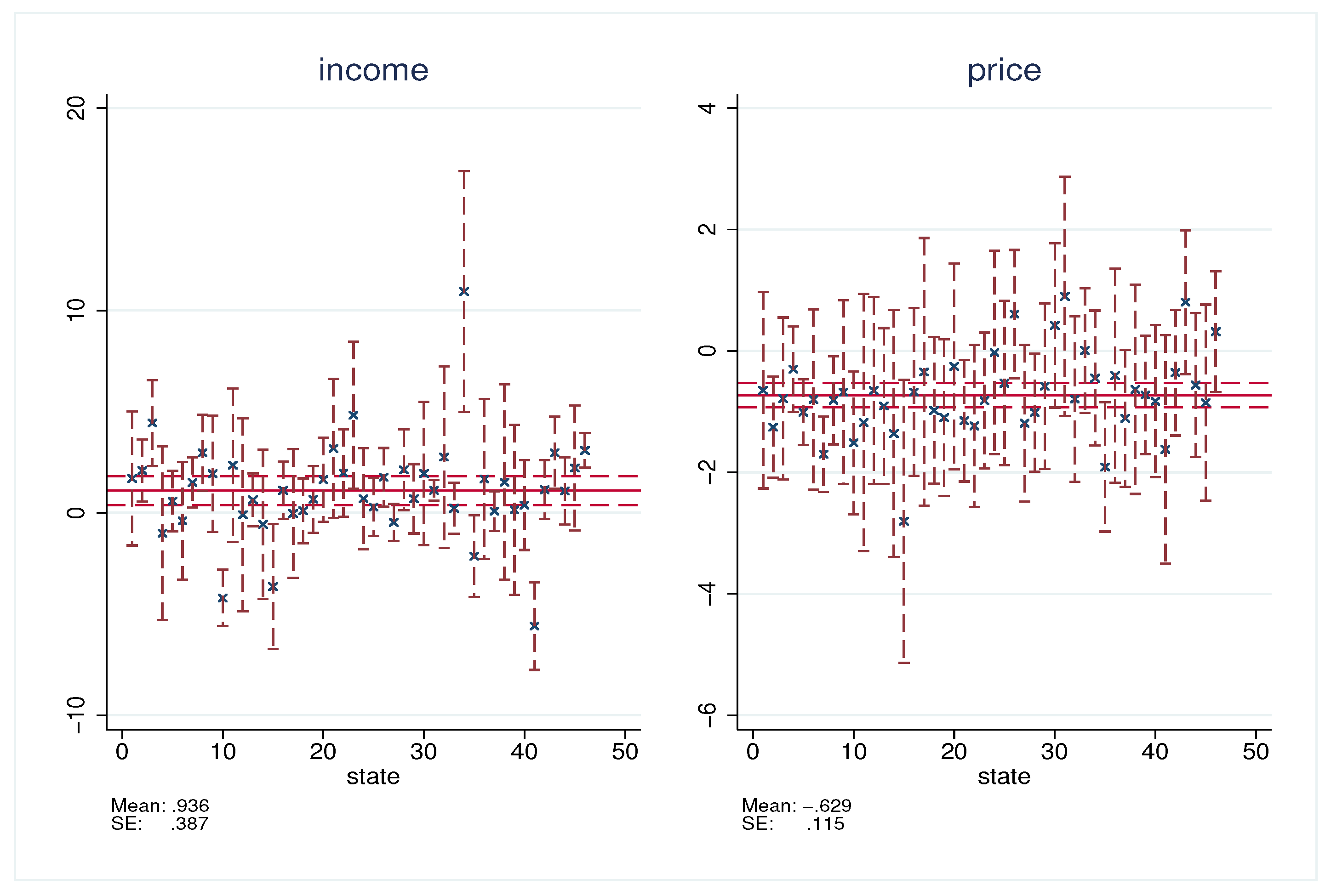
| income | 0.936 | 0.387 | 0.016 | 0.177 | 1.695 |
| price | −0.629 | 0.115 | 0.000 | −0.854 | −0.404 |
Publisher’s Note: MDPI stays neutral with regard to jurisdictional claims in published maps and institutional affiliations. |
© 2022 by the authors. Licensee MDPI, Basel, Switzerland. This article is an open access article distributed under the terms and conditions of the Creative Commons Attribution (CC BY) license (https://creativecommons.org/licenses/by/4.0/).
Share and Cite
Cao, S.; Zhou, Q. Common Correlated Effects Estimation for Dynamic Heterogeneous Panels with Non-Stationary Multi-Factor Error Structures. Econometrics 2022, 10, 29. https://doi.org/10.3390/econometrics10030029
Cao S, Zhou Q. Common Correlated Effects Estimation for Dynamic Heterogeneous Panels with Non-Stationary Multi-Factor Error Structures. Econometrics. 2022; 10(3):29. https://doi.org/10.3390/econometrics10030029
Chicago/Turabian StyleCao, Shiyun, and Qiankun Zhou. 2022. "Common Correlated Effects Estimation for Dynamic Heterogeneous Panels with Non-Stationary Multi-Factor Error Structures" Econometrics 10, no. 3: 29. https://doi.org/10.3390/econometrics10030029
APA StyleCao, S., & Zhou, Q. (2022). Common Correlated Effects Estimation for Dynamic Heterogeneous Panels with Non-Stationary Multi-Factor Error Structures. Econometrics, 10(3), 29. https://doi.org/10.3390/econometrics10030029