Emerging Trends in Optimal Structural Health Monitoring System Design: From Sensor Placement to System Evaluation


Abstract
1. Introduction
2. Overview of the Sensor Placement Optimisation Problem
3. Cost Functions
3.1. Information Theory
3.1.1. Fisher Information
3.1.2. Mutual Information
3.1.3. Information Entropy
3.2. Modal Identification Based Cost Functions
- Sensor quantity: how many sensors are required to enable successful modal identification?
- Sensor placement: where should the available sensors be placed in order to best capture the required data?
- Evaluation: how may the performance of the final, optimised sensor configuration be quantified?
3.2.1. Effective Independence (EI)
3.2.2. Modal Kinetic Energy (MKE)
3.2.3. Average Driving Point Residue (ADPR)
3.2.4. Modeshape Sensitivity
3.2.5. Strain Energy Distribution
3.2.6. Mutual Information
3.2.7. Information Entropy
3.3. SHM Classification Outcomes
3.4. Summary
4. Optimisation Methods
4.1. Sequential Sensor Placement Methods
4.2. Metaheuristic Methods
- generate an initial population (the First Generation) containing randomly-generated individuals. In an SPO context, each ‘individual’ is typically taken to comprise a sensor location subset;
- evaluate the fitness of each individual within the population against a pre-defined cost function;
- produce a new population by (a) selecting the best-fit individuals for reproduction and (b) breeding new individuals through crossover and mutation operations; and,
- repeat steps (2) and (3) above until some stopping criteria is reached.
4.2.1. Genetic Algorithms (GA)
4.2.2. Simulated Annealing (SA)
4.2.3. Ant Colony and Bee Swarm Metaphors
4.2.4. Mixed Variable Programming (MVP)
4.3. Summary
5. Emerging Trends and Future Directions
5.1. From Classifiers to Decisions
5.2. Quantifying the Value of SHM Systems
5.3. Robustness to Benign Effects
5.4. Robustness to Modelling and Prediction Errors
5.5. Robustness to Sensor and Sensor Network Failure
5.6. Scanning Laser Vibrometry
6. Concluding Comments
Author Contributions
Funding
Conflicts of Interest
Abbreviations
| SHM | Structural health monitoring |
| SPO | Sensor placement optimisation |
| DOFs | Degrees of freedom |
| FEA | Finite element analysis |
| EO | Evolutionary optimisation |
| FIM | Fisher information matrix |
| EOV | Experimental and operational variation |
| MAC | Modal assurance criterion |
| NMSE | Normalised mean squared error |
| GA | Genetic algorithm |
| EI | Effective independence |
| SSP | Sequential sensor placement |
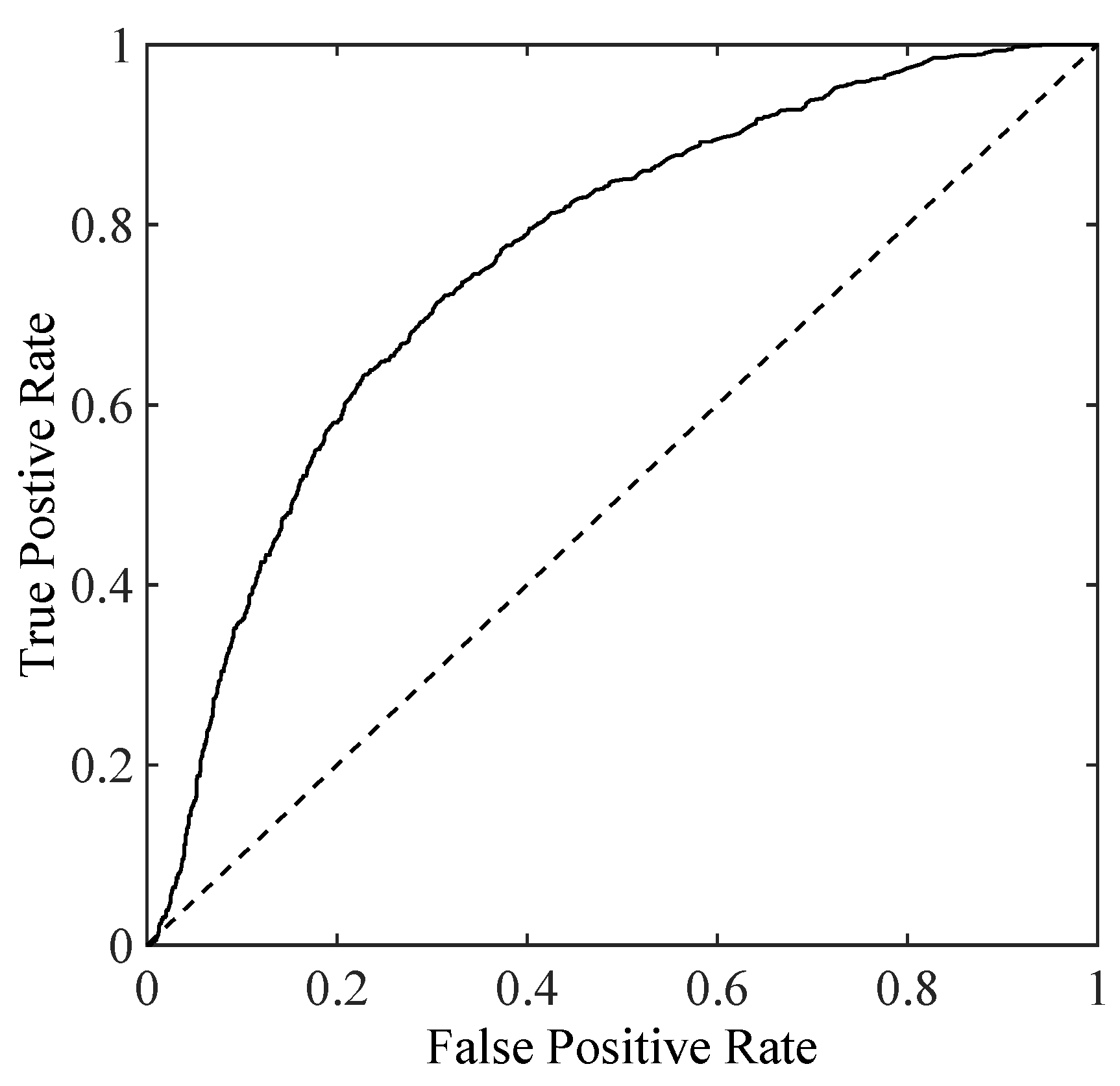
| ROC | Receiver operating characteristic |
References
- Barthorpe, R.J.; Worden, K. Sensor Placement Optimization. In Encyclopedia of Structural Health Monitoring; Boller, C., Chang, F., Fujino, Y., Eds.; John Wiley & Sons: Chichester, UK, 2009. [Google Scholar] [CrossRef]
- Yi, T.H.; Li, H.N. Methodology Developments in Sensor Placement for Health Monitoring of Civil Infrastructures. Int. J. Distrib. Sens. Netw. 2012, 8. [Google Scholar] [CrossRef]
- Ostachowicz, W.; Soman, R.; Malinowski, P. Optimization of sensor placement for structural health monitoring: A review. Struct. Health Monit. 2019, 18, 963–988. [Google Scholar] [CrossRef]
- Papadimitriou, C. Optimal sensor placement methodology for parametric identification of structural systems. J. Sound Vib. 2004, 278, 923–947. [Google Scholar] [CrossRef]
- Udwadia, F. Methodology for Optimum Sensor Locations for Parameter Identification in Dynamic Systems. ASCE J. Eng. Mech. 1994, 120. [Google Scholar] [CrossRef]
- Kammer, D. Sensor placement for on-orbit modal identification and correlation of large space structures. J. Guid. Control. Dyn. 1991, 14, 251–259. [Google Scholar] [CrossRef]
- Shah, P.; Udwadia, F. A Methodology for Optimal Sensor Locations for Identification of Dynamic Systems. J. Appl. Mech. 1978, 45, 188–196. [Google Scholar] [CrossRef]
- Kammer, D. Effect of model error on sensor placement for on-orbit modal identification of large space structures. J. Guid. Control. Dyn. 1992, 15, 334–341. [Google Scholar] [CrossRef]
- Kammer, D. Effects of noise on sensor placement for on-orbit modal identification of large space structures. J. Dyn. Syst. Meas. Control. Trans. ASME 1992, 114, 436–443. [Google Scholar] [CrossRef]
- Yao, L.; Sethares, W.; Kammer, D. Sensor placement for on-orbit modal identification via a genetic algorithm. AIAA J. 1993, 31, 1922–1928. [Google Scholar] [CrossRef]
- Kammer, D. Sensor set expansion for modal vibration testing. Mech. Syst. Signal Process. 2005, 19, 700–713. [Google Scholar] [CrossRef]
- Penny, J.; Friswell, M.; Garvey, S. Automatic choice of measurement locations for dynamic testing. AIAA J. 1994, 32, 407–414. [Google Scholar] [CrossRef]
- Salama, M.; Rose, T.; Garba, J. Optimal placement of excitations and sensors for verification of large dynamical systems. In Proceedings of the 28th Structures, Structural Dynamics and Materials Conference, Monterey, CA, USA, 6–8 April 1987. [Google Scholar] [CrossRef]
- Li, D.S.; Li, H.N.; Fritzen, C.P. The connection between effective independence and modal kinetic energy methods for sensor placement. J. Sound Vib. 2007, 305, 945–955. [Google Scholar] [CrossRef]
- Imamovic, N.; Ewins, D. Optimization of excitation DOF selection for modal tests. In Proceedings of the 15th International Modal Analysis Conference, Orlando, FL, USA, 3–6 February 1997. [Google Scholar]
- Imamovic, N. Validation of Large Structural Dynamics Models Using Modal Test Data. Ph.D. Thesis, Imperial College London, London, UK, 1998. [Google Scholar]
- Larson, C.B.; Zimmerman, D.C.; Marek, E.L. A comparison of modal test planning techniques: Excitation and sensor placement using the NASA 8-bay truss. In Proceedings of the 12th International Modal Analysis Conference, Honolulu, HI, USA, 31 January–3 February 1994; pp. 205–211. [Google Scholar]
- Shi, Z.; Law, S.; Zhang, L. Optimum sensor placement for structural damage detection. J. Eng. Mech. 2000, 126, 1173–1179. [Google Scholar] [CrossRef]
- Guo, H.; Zhang, L.; Zhang, L.; Zhou, J. Optimal placement of sensors for structural health monitoring using improved genetic algorithms. Smart Mater. Struct. 2004, 13, 528–534. [Google Scholar] [CrossRef]
- Hemez, F.; Farhat, C. An energy based optimum sensor placement criterion and its application to structural damage detection. In Proceedings of the SPIE International Society for Optical Engineering, Bergen, Norway, 13–15 June 1994; p. 1568. [Google Scholar]
- Said, W.M.; Staszewski, W.J. Optimal sensor location for damage detection using mutual information. In Proceedings of the 11 th International Conference on Adaptive Structures and Technologies (ICAST), Nagoya, Japan, 23–26 October 2000; pp. 428–435. [Google Scholar]
- Trendafilova, I.; Heylen, W.; Van Brussel, H. Measurement point selection in damage detection using the mutual information concept. Smart Mater. Struct. 2001, 10, 528–533. [Google Scholar] [CrossRef]
- Papadimitriou, C.; Beck, J.; Au, S.K. Entropy-based optimal sensor location for structural model updating. Jvc/J. Vib. Control. 2000, 6, 781–800. [Google Scholar] [CrossRef]
- Tharwat, A. Classification assessment methods. Appl. Comput. Inform. 2018. [Google Scholar] [CrossRef]
- Fawcett, T. An introduction to ROC analysis. Pattern Recognit. Lett. 2006, 27, 861–874. [Google Scholar] [CrossRef]
- Worden, K.; Burrows, A. Optimal sensor placement for fault detection. Eng. Struct. 2001, 23, 885–901. [Google Scholar] [CrossRef]
- Papadimitriou, C. Pareto optimal sensor locations for structural identification. Comput. Methods Appl. Mech. Eng. 2005, 194, 1655–1673. [Google Scholar] [CrossRef]
- Stephan, C. Sensor placement for modal identification. Mech. Syst. Signal Process. 2012, 27, 461–470. [Google Scholar] [CrossRef]
- Stabb, M.; Blelloch, P. A genetic algorithm for optimally selecting accelerometer locations. In Proceedings of the 13th International Modal Analysis Conference, Nashville, TN, USA, 13–16 February 1995; Volume 2460, p. 1530. [Google Scholar]
- Worden, K.; Burrows, A.; Tomlinson, G. A combined neural and genetic approach to sensor placement. In Proceedings of the 15th International Modal Analysis Conference, Nashville, TN, USA, 12–15 February 1995; pp. 1727–1736. [Google Scholar]
- Worden, K.; Staszewski, W. Impact location and quantification on a composite panel using neural networks and a genetic algorithm. Strain 2000, 36, 61–70. [Google Scholar] [CrossRef]
- Coverley, P.; Staszewski, W. Impact damage location in composite structures using optimized sensor triangulation procedure. Smart Mater. Struct. 2003, 12, 795. [Google Scholar] [CrossRef]
- De Stefano, M.; Gherlone, M.; Mattone, M.; Di Sciuva, M.; Worden, K. Optimum sensor placement for impact location using trilateration. Strain 2015, 51, 89–100. [Google Scholar] [CrossRef]
- Overton, G.; Worden, K. Sensor optimisation using an ant colony methapor. Strain 2004, 40, 59–65. [Google Scholar] [CrossRef]
- Scott, M.; Worden, K. A Bee Swarm Algorithm for Optimising Sensor Distributions for Impact Detection on a Composite Panel. Strain 2015, 51, 147–155. [Google Scholar] [CrossRef]
- Beal, J.M.; Shukla, A.; Brezhneva, O.A.; Abramson, M.A. Optimal sensor placement for enhancing sensitivity to change in stiffness for structural health monitoring. Optim. Eng. 2007, 9, 119–142. [Google Scholar] [CrossRef]
- Wolpert, D.H.; Macready, W.G. No free lunch theorems for optimization. IEEE Trans. Evol. Comput. 1997, 1, 67–82. [Google Scholar] [CrossRef]
- Cawley, P. Structural health monitoring: Closing the gap between research and industrial deployment. Struct. Health Monit. 2018, 17, 1225–1244. [Google Scholar] [CrossRef]
- Flynn, E.; Todd, M. A Bayesian approach to optimal sensor placement for structural health monitoring with application to active sensing. Mech. Syst. Signal Process. 2010, 24, 891–903. [Google Scholar] [CrossRef]
- Thöns, S. On the Value of Monitoring Information for the Structural Integrity and Risk Management. Comput. Civ. Infrastruct. Eng. 2018, 33, 79–94. [Google Scholar] [CrossRef]
- Peeters, B.; De Roeck, G. One-year monitoring of the Z24-Bridge: Environmental effects versus damage events. Earthq. Eng. Struct. Dyn. 2001, 30, 149–171. [Google Scholar] [CrossRef]
- Kullaa, J. Eliminating Environmental or Operational Influences in Structural Health Monitoring using the Missing Data Analysis. J. Intell. Mater. Syst. Struct. 2009, 20, 1381–1390. [Google Scholar] [CrossRef]
- Cross, E.J.; Worden, K.; Chen, Q. Cointegration: A novel approach for the removal of environmental trends in structural health monitoring data. Proc. R. Soc. A 2011, 467, 2712–2732. [Google Scholar] [CrossRef]
- Li, D.S.; Li, H.N.; Fritzen, C.P. Load dependent sensor placement method: Theory and experimental validation. Mech. Syst. Signal Process. 2012, 31, 217–227. [Google Scholar] [CrossRef]
- Papadimitriou, C.; Lombaert, G. The effect of prediction error correlation on optimal sensor placement in structural dynamics. Mech. Syst. Signal Process. 2012, 28, 105–127. [Google Scholar] [CrossRef]
- Castro-Triguero, R.; Murugan, S.; Gallego, R.; Friswell, M.I. Robustness of optimal sensor placement under parametric uncertainty. Mech. Syst. Signal Process. 2013, 41, 268–287. [Google Scholar] [CrossRef]
- Side, S.; Staszewski, W.; Wardle, R.; Worden, K. Fail-safe sensor distributions for damage detection. In Proceedings of the DAMAS’97 International Workshop on Damage Assessment using Advanced Signal Processing Procedures, Sheffield, UK, 30 June–2 July 1997; pp. 135–146. [Google Scholar]
- Kullaa, J. Distinguishing between sensor fault, structural damage, and environmental or operational effects in structural health monitoring. Mech. Syst. Signal Process. 2011, 25, 2976–2989. [Google Scholar] [CrossRef]
- Bhuiyan, M.; Wang, G.; Cao, J.; Wu, J. Deploying Wireless Sensor Networks with Fault-Tolerance for Structural Health Monitoring. IEEE Trans. Comput. 2015, 64, 382–395. [Google Scholar] [CrossRef]
- Yi, T.H.; Huang, H.B.; Li, H.N. Development of sensor validation methodologies for structural health monitoring: A comprehensive review. Measurement 2017, 109, 200–214. [Google Scholar] [CrossRef]
- Staszewski, W.; Lee, B.; Mallet, L.; Scarpa, F. Structural health monitoring using scanning laser vibrometry: I. Lamb wave sensing. Smart Mater. Struct. 2004, 13, 251. [Google Scholar] [CrossRef]
- Marks, R.; Clarke, A.; Featherston, C.A.; Pullin, R. Optimization of acousto-ultrasonic sensor networks using genetic algorithms based on experimental and numerical data sets. Int. J. Distrib. Sens. Netw. 2017, 13. [Google Scholar] [CrossRef]
- Gardner, P.; Liu, X.; Worden, K. On the application of domain adaptation in structural health monitoring. Mech. Syst. Signal Process. 2020, 138, 106550. [Google Scholar] [CrossRef]


| Predicted Class | |||
|---|---|---|---|
| Positive | Negative | ||
| Actual Class | Positive | TP | FP |
| Negative | FN | TN | |
| Predicted Location | ||||
|---|---|---|---|---|
| A | B | C | ||
| Actual Location | A | |||
| B | ||||
| C | ||||
© 2020 by the authors. Licensee MDPI, Basel, Switzerland. This article is an open access article distributed under the terms and conditions of the Creative Commons Attribution (CC BY) license (http://creativecommons.org/licenses/by/4.0/).
Share and Cite
Barthorpe, R.J.; Worden, K. Emerging Trends in Optimal Structural Health Monitoring System Design: From Sensor Placement to System Evaluation. J. Sens. Actuator Netw. 2020, 9, 31. https://doi.org/10.3390/jsan9030031
Barthorpe RJ, Worden K. Emerging Trends in Optimal Structural Health Monitoring System Design: From Sensor Placement to System Evaluation. Journal of Sensor and Actuator Networks. 2020; 9(3):31. https://doi.org/10.3390/jsan9030031
Chicago/Turabian StyleBarthorpe, Robert James, and Keith Worden. 2020. "Emerging Trends in Optimal Structural Health Monitoring System Design: From Sensor Placement to System Evaluation" Journal of Sensor and Actuator Networks 9, no. 3: 31. https://doi.org/10.3390/jsan9030031
APA StyleBarthorpe, R. J., & Worden, K. (2020). Emerging Trends in Optimal Structural Health Monitoring System Design: From Sensor Placement to System Evaluation. Journal of Sensor and Actuator Networks, 9(3), 31. https://doi.org/10.3390/jsan9030031