1. Introduction
A wireless sensor network (WSN) is a distributed system consisting of several nodes, and one or more base stations (BS). The nodes are typically small and cheap. BS’s have higher processing capabilities and a wired electrical power source. The sensor nodes are equipped with application-specific sensors and a mini central processing unit. There is also a wireless radio transceiver attached to each sensor node; it provides the node with the capability to communicate with each other and with the BS. These nodes often operate on their battery power and use unreliable radio channels corrupted by noise and fading. As a result, the primary concern, when designing and operating such a network, is to maximize the life span and the data throughput of the nodes [
1].
Packets are sent to the BS either in a single-hop manner or in a multi-hop manner. In case of single hop, the node sends the generated packet directly to the base station, wherein a multi-hop manner, source nodes send packets to BS via multi-node path, each node of the path forwards the received (or, in the case of the source node, the generated) packet to another node until the BS receives the packet [
2]. Packets are transmitted to the BS via unreliable radio channels corrupted by noise and fading [
3].
Many techniques have been developed to increase the energy efficiency of WSNs, covering almost all layers of communication protocols ranging from the physical layer to the application layer [
4,
5]. Routing is instrumental when designing and operating WSNs; the researchers in [
6] describe a group of routing metrics and constraints; they provide a guideline for the composition of these metrics to achieve efficient routing schemes.
Load balancing and reliable information transfer are contributory factors in energy-efficient communications. Lack of load balancing causes the death of some nodes too early, which breaks the connectivity of WSN and reduces the life span of the WSN [
7]. The lifespan is defined as the length of time interval until the first node goes flat [
8].
The reliability in WSN categorized into three classes: packet reliability, event reliability, and packet-event reliability. In this paper, we focus on packet reliability. It is classified to up-stream packets, (which mostly represents data packet), and down-stream packets, (which generally represent control packets) [
3]. Low reliability leads to high packet loss ratio in the case of low energy consumption. Most protocols achieve energy efficiency by enforcing uniform energy distribution and maximum longevity, but they do not provide reliable links where lost data means wasted energy. Also, they don’t use distinct measure for the uniformity of residual energy distribution.
In this paper, we try to strike a good balance between reliability and energy consumption (longevity). Our concern in the first part of this paper is to develop novel routing algorithms that maximize the minimum residual energy subject to a predefined reliability target. To achieve this, we propose the Maximum of the Minimum Residual Energy Protocol (MMREP). According to the proposed method, we select a path by which a packet is sent to the BS over the nodes, of which the minimum remaining energy is the maximum subject to the reliability constraint. The reliability constraint means that the packet will reach the BS with a given probability. This strategy can significantly extend the life span of WSNs.
In the second part of this paper, we improve the performance of the basic MMREP in terms of energy efficiency and complexity. We propose an Optimal Residual Energy Based Protocol (OREBP). In OREBP, we use the entropy-like function to measure the uniformity of the residual energy distribution. The packets are sent to the BS in a multi-hop manner. The protocol guarantees that the distribution of the residual energy will remain as close to uniform as possible. We will demonstrate that this method achieves optimal load balancing.
In this paper, we introduce two novel routing algorithms. They achieve an efficient load balancing under predefined reliability constraint. The key contributions of this paper are summarized as follows: First, we presented a mathematical analysis for the selection of relay nodes based on the remaining energy and reliability. Second, we proposed MMREP to select the path that maximizes the remaining energy of its nodes subject to the reliability constraint. Third, we introduced the entropy-like function to measure the uniformity of residual energy distribution. Fourth, we proposed OREBP, which selects the path based on the entropy of residual energy of the path.
The remainder of the paper is organized as follows:
In
Section 2, we provide an overview of related work in the literature.
In
Section 3, we introduce the framework in which the different communication protocols will be discussed.
In
Section 4, we describe MMREP to select the path which keeps the residual energy as maximum as possible.
In
Section 5, we describe OREBP to select the optimal path that maintains uniform residual energy distribution.
In
Section 6, we give the numerical results of a detailed performance analysis of the algorithms where their performances are compared with other protocols.
In
Section 7, some conclusions are drawn, and remarks on future research directions are given.
2. Related Work
Previous works were done in the field, classify energy-efficient routing protocols into homogeneous WSN protocols (where all the nodes are identical) and heterogeneous WSN protocols, where both are subdivided into static and mobile [
9]. Other researchers classify them based on network structure (flat and hierarchical); communication model (negotiation-based, query-based, and coherent-based); topology (location-based and mobile agent-based); and reliability (QoS-based and multipath-based) [
10].
Some researchers improved the energy efficiency of WSN by using hierarchical packet forwarding protocols. Low Energy Adaptive Clustering Hierarchy (LEACH) is a hierarchical cluster-based protocol. The network is divided into several clusters; a cluster head (CH) is selected to receive the packets from respective members of that cluster, and then, it forwards the packet directly to the BS. In LEACH, energy efficiency is achieved by clustering and data fusion. By clustering, just the CH has a direct long-distance transmission to the BS; other nodes send their data to CH in short-distance transmission. By data fusion, the CH removes redundant data and fuses the received packets into a single packet. The cluster heads are selected randomly and changed periodically in time to achieve load balancing [
11]. However, ignoring the energy level of the cluster head may make it a bottleneck node, and it does not consider reliability.
There are several modified versions of LEACH, these modifications based on three titles, selection of CH, clustering, and data transmission. In LEACH-C, the selection of CH is centric and performed by BS based on the remaining energy and location of nodes [
9]. In NEAHC, load balance and energy efficiency are achieved by selecting the CH based on remaining energy. Also, members with low energy are forced to switch between sleep and active status [
12]. The authors of [
13] propose the selection of CH and clustering based on practical swarm optimization and fuzzy logic; the fitness function depends on the distance between nodes and CH, the distance between CH and BS, and the minimum consumed energy. In [
14], the firefly heuristic algorithm is used to select the CH based on distance, energy, and delay. In terms of clustering, CACD algorithm constructs clusters based on the energy depletion of the clusters and node density [
15].
PEGASIS is an underlying chain-based routing protocol [
16], it is a modification of LEACH, the nodes are grouped into a chain using a greedy algorithm, and each of them acts as chain head in turn; each node fuse the received packet into its packets, the fused packet is forwarded to the closest neighbor until it arrives at the chain leader. The chain leader aggregates the packets together and sends them directly to the BS. By selecting the chain leader, regardless of its energy, can result in a shorter lifespan. CHIRON [
17] is a chain-based routing protocol that increases energy efficiency by dividing the network field into some smaller areas to create shorter chains for reducing data transmission delay and path duplication. The Energy-Efficient Chain-Based (EECB) routing protocol [
18] modified PEGASIS by selecting the chain leader based on the residual energy and distance from the BS. The scheme in [
19] selects the chain leaders from a group of nodes in the neighborhood of BS. The authors of [
20] used a heuristic Ant Colony optimization to reduce delay and to find the optimal path with minimum transmission distance.
Regarding the reliability, in [
8], an energy-efficient and reliable protocol is proposed, predefined reliability is achieved by multipath routing. But, only two-hop paths are assumed. Researchers of [
21], improve the reliability by finding the best location of CH. RE-AEDG [
22] and GIN [
23] protocols use the cooperative routing model to enhance reliability, where the transmitted packet is overheard by several neighbors and retransmitted by several neighbors too. Some researches use network coding to improve reliability [
24,
25]. Most of these protocols improve reliability by increasing the redundant data, which means wasted energy.
These protocols, however, do not achieve optimal energy balancing, and do not take the reliability into consideration when selecting an energy-efficient path. As a result, further investigation is needed into developing packet forwarding mechanisms.
3. The Model
WSNs consist of a number of nodes which are deployed randomly in a sensing field. The network is represented by a graph , where set refers to the nodes , while set denotes the edges and are the distances between the nodes, which are arranged in a distance matrix, and the distance represents the weight of the corresponding edge. Packets are forwarded from the nodes to the BS in the form of multi-hop routing. In multi-hop protocols, the nodes use each other to relay the packets until packet is finally received by the BS.
Based on the Rayleigh fading model [
18], the energy
needed for transmitting a single packet over distance
with the probability of successful transmission between node
and node
denoted by
is given as:
where
is the so-called modulation and coding constant [
26],
denotes the power of noise,
is the large-scale path loss exponent (usually
).
The reliability constraint is expressed by a predefined data loss percentage ; where the probability of overall success of packet transmission from the source node to the BS is supposed to fulfil , in case of using relay nodes to forward packets to the BS. We adjust to get same for all nodes, then .
The energy of the network at time is described by an energy state vector where represents the available battery power at node at time instant . We assume that all the nodes have the same initial energy at time instant , i.e., . When seeking a path for a maximum relay node from the source node to the BS, we search for a set of indices referring to the relay nodes participating in the packet transfer, where the first source node, , sends the packet to node then the packet is forwarded to node and so on, and finally from node to the BS. Each node has a copy of the routing table which is calculated and broadcasted by the BS.
In the forthcoming discussion, we assume that the BS has full information on the distance matrix of the network and, as a result, it has the routing table of all nodes. The BS updates its version of the energy state vector after receiving each packet, by which it perceives of the remaining energy and the existence of the nodes. With each round, it runs the proposed algorithms to calculate the optimal path from each node according to the energy state vector, the predefined data loss percentage , and predefined maximum number of hops. The updated routing table is then broadcast to all nodes. We also suppose deterministic transmission, where the nodes transmit the same amount of data in a predefined frequency (periodically), and each node forwards packets according to its routing table.
One may say that this procedure will increase the energy consumption due to the frequency of BS broadcasting. However, the energy needed for receiving is significantly less than the energy needed for transmission [
15]; it does not depend on the distance; it just depends on the size of the received information. The information received by the nodes is a short control message; it consists of the ID of the node, the ID of the next relay node, and the ID of the source node. Moreover, nodes eliminate the overhead required for chain or path setup, as with PEGASIS and LEACH [
8,
15]. The BS, with its high energy and high computational capabilities, does all the work—this configuration is used for the majority of IoT systems. Besides that, the proposed algorithms reduce the consumed energy in overhearing reception; the node receives just from the relay node specified by BS deterministically, which makes the algorithms beacon-less because the nodes don’t need to exchange routing information.
In the proposed protocols, aside from the necessity of determining the optimal energy consumption values that maximizes the residual energy of the path, it is also necessary to guarantee that the packets arrive at the BS with a given reliability
4. Maximizing the Minimal Residual Energy
In this section, we select a path by which a packet is sent to the BS with the minimum remaining energy is maximum subject to the constraint that the packet will reach the BS with a given probability.
Thus, the path over which the packet is forwarded to the BS (denoted by
) is optimal if:
subject to the constraint
. This strategy can be implemented when the hop count of packet transfer has been set prior to sending the packet to the BS.
4.1. Two-Hop Routing
Let us assume that packets are forwarded to the BS in a two-hop path, and the sender node is denoted by
, while the intermediate node relaying this packet to the BS is denoted by
. Then, there are two components that change in vector
compared to
,
and
Furthermore, to ensure that the packet sent by node
reaches the BS with a given probability
, then the reliability constraint can be expressed
. Thus, in the case of two-hop routing, one can determine the relay node
, by solving the following constrained optimization problem:
subject to the constraint
.
Solution
Let us assume that we have chosen a relay node denoted by index
, then the condition
can be paraphrased as:
From Equation (6), we can define
which expresses the relationship between
and
due to the constraint as:
The minimum residual energy (if node
is selected) will be maximum if the residual energy at the source node and the relay node are equal to each other, i.e.,
. So, from Equations (2) and (3):
and by using Equations (6) and (7), we have:
We can use Equation (8) to determine
. Since the source node
is given, we can calculate
for all possible relay nodes
. Then
can be selected by solving the problem:
This requires the solution of (8) times and then comparison of the value .
4.2. m-Hop Routing
Based on this reasoning, the protocol can easily be extended to m-hop routing as well. In this case, we assume that packets are forwarded to the BS via an m-hop path and the sender node is node and the sink node is the BS denoted by . The path containing the sender and the relay nodes is denoted by .
Then, there are m + 1 components changing in vector compared to , given as , j = 0, …, m. Similar to the previous constraint, if we want to ensure that the packet sent by node reaches the with a given probability , then the reliability constraint can be expressed as .
Thus, in the case of m-hop routing, we have to solve the following constrained optimization problem:
subject to the constraint
.
Solution
Let us assume that we have chosen a path . Along with this path, the reliability constraint can alternatively be given as .
From Equation (1) it becomes:
The minimum residual energy will be maximum if the residual energy at all the relay nodes are equal to each other, i.e.,
. So, from Equations (2) and (3):
The
equations above yield a solution to
. We can calculate
for all possible m-hop paths by fixing the path
. Then the optimal path
can be sought by solving the following problem:
This requires the solution of (11) times and then comparisons of the value . We will refer to this method of routing the packets to the BS as the maximum of minimum residual energy protocol (MMREP).
5. Optimal Path Selection Based on Energy Entropy
We can further generalize this method by introducing an entropy-like measure on energy distribution. The equality of residual energy of relay nodes can be extended for uniform distribution of residual energy across all the path’s nodes. This uniformity can be achieved by maximizing entropy. At instant
, the entropy is maximum because all the nodes have the same initial energy; to keep the entropy at maximum, the gradient of the entropy should be minimized. We can calculate the entropy of the normalized residual energy distribution on the nodes of the network
at time instant
. Hence, the entropy characterizing the current energy distribution is:
The gradient of the entropy can be calculated as follows:
Suppose that source node
is sending a packet via the relay nodes
where
is the last relay node, then the residual energy of nodes involved in packet forwarding will change as:
Further, the gradient of the entropy of the power distribution on a relay node is given as:
While the gradient of the entropy of the power distribution on the other nodes of the path is given as:
Thus, the change of the entropy is:
The optimal path is the one that keeps this gradient minimum, thus enforcing only small changes in the energy entropy, guaranteeing that the energy distribution falls as close to its maximum as possible. In this way, a more or less uniform residual energy distribution can be maintained while sending packets to the BS. The optimum choice of relay nodes (i.e., the optimal path) which minimizes the change in the gradient can thus be obtained as:
After each round, the BS updates the residual energy vector of all nodes, , finds the optimal path from node to the BS, and calculates the relay nodes of the path using OREBP. The BS broadcasts a new look-up-table containing the optimal routes of each node. This can help reduce the computational load on the nodes and improve their energy efficiency.
We will refer to this method of routing the packets to the BS as the Optimal Remaining Energy-Based Protocol (OREBP). The needed calculations increase as the number of maximum hops () increases; as the maximum number of hops () increases, more possible paths are available and more optimality is achieved.
6. Simulation Results
The performance of the proposed algorithms MMREP and OREBP, respectively are evaluated in comparison to the PEGASIS protocol. In PEGASIS, each node forwards the packet to its closest neighbor; when the packet arrives at the chain leader, it sends the packet directly to the base station.
PEGASIS does not take reliability into consideration, whereas MMREP and OREBP do. To introduce reliability constraints to PEGASIS and thus make it comparable with the proposed protocols, it is modified as follows: each packet should be forwarded to the BS with at least success probability
, where
is the source node and
is the destination node. From Equation (1)
,
is calculated as in [
26]. In case of an
-hop path,
. For the whole round, we will calculate the average success probability of all paths.
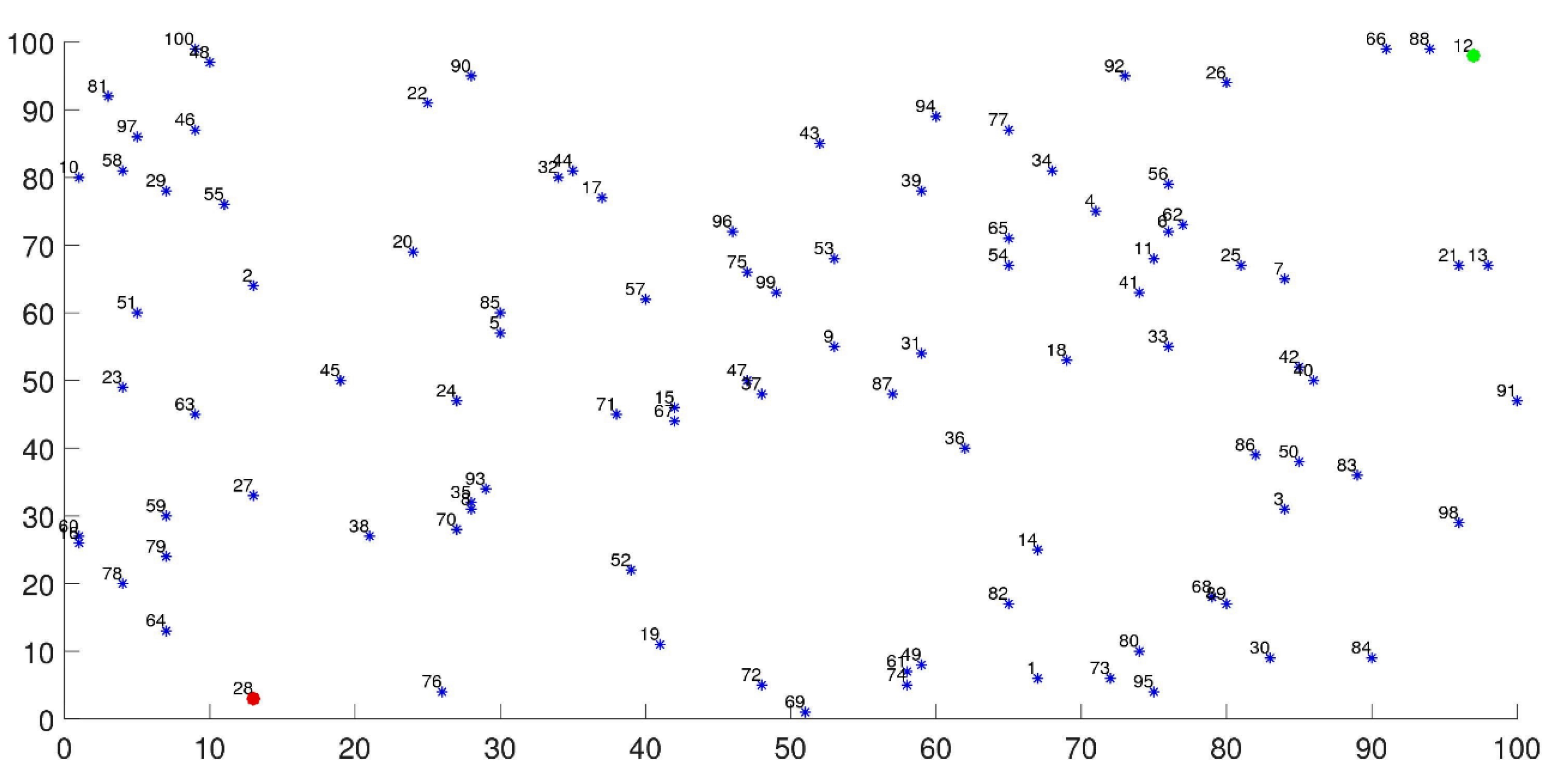
Figure 1 shows how 100 nodes are deployed randomly onto a grid of 100 m × 100 m according to a 2D normal distribution; the BS is allocated in the upper-right corner of the sensing field, as shown by the green point. while
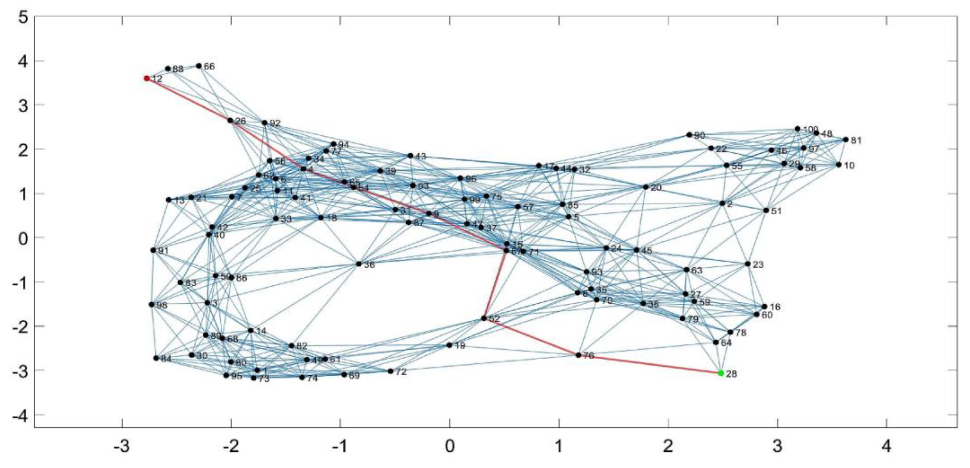
Figure 2 shows the network as a graph. The highlighted chain is constructed by the Dijkstra shortest path algorithm, as defined by the base station.
The transmission energy will be calculated according to the Rayleigh fading model (1) under the following assumptions:
We neglect the conditioning energy needed by the electronics.
is calculated based on reliability and the number of relay nodes , where . We assume that is the same for all nodes, then .
All the nodes have the same initial energy.
The life span is the number of packets transmitted over the chain until the first node goes flat. Each transmission round carries a single packet.
Each node has an adjustable power transmission, which enables it to access any node in the chain including the BS.
The path shown in
Figure 2 consists of seven nodes, numbered from 1 to 7, where node number 1 is the farthest from the BS, it shown as red point in
Figure 1.
Figure 3 shows the residual energy of the nodes of the chain for MMREP, OREBP, and PEGASIS respectively, when the first node goes flat. In the case of MMREP and OREBP, we note that almost all the nodes have the same level of residual energy, the residual energy is distributed more uniformly (near zero) for all nodes, In the case of PEGASIS, we note that as the node gets further away from the BS, it loses energy at a higher rate, the residual energy of the nodes decreases as the nodes gets farther from the BS. So, we note unevenly distribution of the residual energy.
Figure 4 shows the life span of a network which uses MMREP, OREBP, PEGASIS, subject to a reliability constraint, with different data loss percentage ε values, 0.025, 0.05, 0.075, 0.01, 0.125 and 0.15, respectively. Since PEGASIS does not consider ε when calculating transmission energy, the figure shows that it has a higher life span than MMREP and OREBP; it uses lower transmission energy, which causes a higher packet loss percentage, which means lower reliability; hence, the life span of a network with PEGASIS is the same regardless of data loss percentage ε. In the case of the proposed algorithms, however, life span increases with increasing data loss percentage ε, while the probability of successful packet transmission (1-ε) is decreasing. With MMREP and OREBP, the life span is a function of ε. The users can trade-off between the reliability represented by ε and the life span.
Figure 5 shows the success probability with OREBP and PEGASIS. We assume a predefined data loss rate
for OREBP. The success probability for PEGASIS is calculated as mentioned above. The figure shows the success probability against a variable number of hops ranging from one to six. OREBP always has a higher success probability than PEGASIS, although the value depends on the number of hops. The figure shows that using OREBP improves the reliability from 63% in case of a one-hop path to 71% in case of a six-hop path. Lost data means wasted energy. The figure shows that the success probability decreases with an increasing number of hops. In OREBP, we can control the success probability by trading off between predefined data loss
with life span, as shown in
Figure 4.
Figure 6 shows the relationship between the life span and the number of hops with MMREP, OREBP, and PEGASIS. We assume a predefined data loss rate (ε = 0.05). In the case of MMREP, OREBP, the consumed energy depends on ε. The probability of the overall success of packet transmission from the source node to the BS should satisfy
, where
is the number of the hops. The figure shows the life span against a variable number of hops ranging from one to four. We note that the life span with OREBP increases as the number of hops increases. But, in the case of MMREP, the relationship is unstable because the set of Equations (11) is solved numerically, where a set of solutions are found, so, one needs an algorithm to pick the suitable solution. In OREBP, life span increases as the number of maximum hops increases because there are more paths available to select from. With PEGASIS, the consumed energy is a function of single transmissions rather than the path overall transmissions, so it does not depend on the number of hops.
As the number of hops increases, not only the life span increases, but also the complexity of the algorithm increases.
Figure 7 shows the relationship among the maximum number of hops
, on the
x-axis, the life span
y-axis on the left, and the execution time (a proxy for the complexity) on the secondary
y-axis on the right. As expected, the figure shows that in OREBP as the number of hops increases, the life span increases, but the complexity of the protocol also increases. The user has the choice of trade-offs between the life span, the complexity, and the maximum number of hops.
All the figures show higher a life span with PEGASIS, but also a high percentage of lost data, which implies wasted energy. The results show that the performance of OREBP is better than the performance of MMREP. As we mentioned, MMREP is the basic idea of the algorithm, but we used the entropy principle to optimize it and to reduce its complexity.
7. Conclusions
In this paper, we introduced a protocol which maximizes the minimum residual energy subject to a predefined reliability constraint. We optimized the energy balancing of WSNs by a new protocol (OREBP) to achieve uniform energy consumption by maximizing an entropy-like measure. As demonstrated by the simulation results, the proposed protocols improve the energy efficiency of WSNs by maximizing the life span, subject to a reliability constraint. They also improve the energy consumption distribution among the nodes of the network. The performance of the proposed protocols is compared to the performance of PEGASIS. As shown, the proposed protocols still have a high degree of complexity. We defined four performance parameters: life span, data loss percentage, the maximum number of hops, and the complexity. The user has the choice to control the performance by striking an optimal trade-off among these parameters. To achieve this requires a solution of a complicated optimization problem.
