Article

Performance Comparison of Closed-Form Least Squares Algorithms for Hyperbolic 3-D Positioning

by
Mohamed Khalaf-Allah
Institute of Traffic Telematics, Technische Universität Dresden, 01062 Dresden, Germany
J. Sens. Actuator Netw. 2020, 9(1), 2; https://doi.org/10.3390/jsan9010002
Submission received: 19 November 2019 / Revised: 13 December 2019 / Accepted: 15 December 2019 / Published: 20 December 2019
(This article belongs to the Special Issue Localization in Wireless Sensor Networks)

Abstract

:
An accurate 3-D wireless local positioning system (LPS) is a highly demanded tool for increasing safety in, e.g., emergency response and security operations. An LPS is an attractive approach that can meet stringent requirements and can achieve acceptable accuracies for a long time during extended operations in global navigation satellite system (GNSS)-denied environments. In this work, three closed-form (CF) least squares (LS) algorithms were considered, where two of them were adapted to exploit the knowledge about nuisance parameters for accurate 3-D positioning based on time difference of arrival (TDoA) measurements. The algorithms utilize the single set (SS) of the TDoA measurements, an extended SS (ExSS) of the TDoA measurements, or the full set (FS) of the TDoA measurements, and were denoted, respectively, as the CFSSLS, CFExSSLS, and CFFSLS solutions. The performance of the algorithms was investigated with simulations and real-world measurements, where the wireless system transmitters were placed in a quasi-coplanar arrangement. At moderate to high signal-to-noise ratio (SNR) levels, the CFSSLS solution has the best performance, followed by the CFExSSLS solution and then by the CFFSLS solution. At low SNR levels, the CFFSLS algorithm outperformed the other two algorithms. Both the CFSSLS and CFFSLS solutions estimate nuisance parameters that are utilized in refining the vertical position estimate of the receiver. The CFFSLS solution delivers more accurate refined vertical position estimates since it utilizes more nuisance parameters, i.e., more information. The experimental results confirmed the simulation study in which the CFFSLS algorithm outperformed the other two algorithms, where the experimental environment was dominated by total non-line-of-sight (NLoS) conditions and low SNR levels at the receiver to be located. Therefore, it is recommended to use the FS TDoA measurements for 3-D positioning in bad signal conditions, such as high noise levels and NLoS propagation.

1. Introduction

Determining the position of a receiver based on signal measurements from an array of spatially separated transmitters with well-known locations has been, and is still, an important issue in wireless sensor networks, mobile communications, radar, sonar, and global navigation satellite system (GNSS) applications. Position information is also the key enabler for a constantly increasing number of innovative services and applications. New applications increase the demand for positioning systems where the GNSS signals are denied, e.g., indoors. Current local positioning systems (LPSs) may fail to meet the requirements of certain applications such as indoor emergency operations, e.g., fire-fighting, security and military missions, due to the need for a pre-installed radio frequency (RF) infrastructure. The rapid deployment of a portable infrastructure for positioning during emergency operations may not allow us to carry out extensive calibrations and signal characterization in the target environment, in order to optimize positioning algorithms and increase their position solution accuracy.
RF-based LPSs use wireless technologies to estimate the position of the receiver in areas where no GNSS reception is available. Therefore, positioning based on wireless technologies is an active research area. The commonly used signal measurements for positioning, i.e., location-dependent parameters, include time measurements, i.e., time of arrival (ToA), time difference of arrival (TDoA), and round-trip time of flight (RToF), phase measurements, i.e., phase of arrival (PoA) and phase difference of arrival (PDoA), frequency-based measurements, i.e., signal Doppler frequency (SDF) and frequency difference of arrival (FDoA) (also called differential Doppler (DD)), received signal strength (RSS), and angle of arrival (AoA) of the transmitted signal in addition to hybrid signal measurements, e.g., ToA/RSS, ToA/AoA or TDoA/FDoA. Distance information or range between the receiver and the transmitters can be extracted from ToA, TDoA, RToF, PoA, PDoA, and RSS measurements. The nonlinear relationships of these measurements with the receiver’s position render positioning a nontrivial task.
ToA techniques use the signal propagation time to calculate the distance between the transmitter and the receiver, provided the signal propagation speed in the medium is known [1]. Strict synchronization between transmitters and the receiver is required. The TDoA method exploits the difference in signals’ propagation times from different transmitters, measured at the receiver. Synchronization is required only between the transmitters. The positioning accuracy of ToA and TDoA approaches depends on the signal bandwidth and sampling rate at the receiver. The accuracy degrades in non-line-of-sight (NLoS) conditions. RToF measures the round-trip, i.e., transmitter–receiver–transmitter, signal propagation time to estimate the distance. Therefore, only moderate clock synchronization between the transmitters and the receiver is required. RToF estimation accuracy is also affected by the sampling rate and signal bandwidth, but even more severely due to the two-way signal propagation. Moreover, the response delay at the receiver further deteriorates the accuracy [1].
Phase measurement approaches exploit the phase or phase difference of the carrier signal to estimate the distances between the transmitters and the receiver. The transmitted signals are commonly assumed to be purely sinusoidal, having the same frequency and zero phase offset [2]. Line-of-sight (LoS) conditions are required for high positioning accuracy.
Techniques for radio source location based on the Doppler effect include SDF and FDoA approaches. SDF methods [3] estimate the Doppler frequency shifts in received signals from radio sources and can be implemented by a single portable receiver. Spectrum analysis techniques enable the simultaneous localization of multiple radio sources [4]. In FDoA methods [5], the signal of a stationary radio source is intercepted by at least two moving receivers, and the frequency difference between the receivers is measured at several positions along their trajectories in order to determine the radio source location. For accurate FDoA estimates, the receivers’ frequencies have to be precisely synchronized.
The RSS-based approach is a simple, cost-efficient, and widely used method [6]. The actual signal power strength received at the receiver is used to estimate the distance to the transmitter, where the higher the RSS value the smaller the distance. The positioning accuracy is generally poor due to multipath fading and especially in NLoS situations.
AoA-based approaches use antenna arrays [7] at the receiver side. The TDoA at individual elements of the array are calculated to estimate the angle at which the transmitted signal impinges on the receiver. AoA-based positioning provides accurate estimation at small transmitter–receiver distances. With increasing distances and multipath effects, the accuracy deteriorates significantly.
Most positioning systems use the conventional suboptimal two-step approach, in which measurements, i.e., location-dependent parameters, are first extracted from the signals and then used for position determination. On the other hand, direct position determination (DPD) [8,9,10] performs positioning in a single step and without first estimating the location-dependent parameters. However, the DPD often needs to minimize a nonconvex cost function in order to estimate the position, which demands high computational resources.
The focus in this article is on conventional hyperbolic positioning, i.e., TDoA-based positioning, where the position fix is computed from a set of intersecting hyperbolic curves generated by TDoA measurements. A summary of the most popular circular, i.e., ToA-based, and hyperbolic positioning algorithms is presented in ref. [11]. When the positioning algorithm assumes an additive measurement error model, the available approaches include the maximum likelihood (ML) and the least squares (LS) approaches, which are implemented as iterative or non-iterative, i.e., closed-form (CF) algorithms. The nonlinear hyperbolic equations were linearized by using the Taylor series expansion and solved iteratively in [12,13] using the LS estimator (LSE). If the initial guess of the position estimate is not accurate enough, the convergence to the global solution cannot be guaranteed. Gradient-based techniques, such as the quasi-Newton technique [14] and the Gauss–Newton-type Levenberg–Marquardt method [15], have also been used in iterative algorithms. The ML solution to the hyperbolic equations [16] is widely used due to the proven asymptotic consistency and efficiency of the ML estimator (MLE), which requires assumptions about the distribution of measurement errors. However, the iterative algorithm to find the solution is computationally intensive.
In this article, three CF LS algorithms, i.e., closed-form single set least squares (CFSSLS) [17], closed-form extended single set least squares (CFExSSLS), which is based on the direct method (DM) algorithm in ref. [18], and closed-form full set least squares (CFFSLS) [19], are presented to estimate the 3-D position of a receiver using wireless signal TDoA measurements. Two algorithms, namely, CFSSLS and CFFSLS, estimate nuisance parameters. Therefore, both algorithms are extended, according to refs. [19,20], respectively, to benefit from the nuisance parameter information in refining, i.e., minimizing the error in, the vertical position estimates. Moreover, a design parameter is introduced to control the amount of nuisance parameter information to be used. The DM algorithm in ref. [18], which requires exactly five transmitters, is extended to work with an arbitrary number of transmitters, i.e., N 5 , in order to obtain an LS position solution called the CFExSSLS algorithm. With coplanar transmitters, only 2-D position estimates can be obtained. To obtain 3-D position estimates, a height sensor might be required, or transmitters have to be placed at enough different heights to create the necessary good geometry for 3-D positioning. Simulations and experiments are carried out to confirm the capacity of the adapted algorithms to obtain 3-D position estimates with coplanar transmitters in challenging wireless signal conditions and without any extra sensors.
The rest of the article is organized as follows. Related work is discussed in Section 2. In Section 3, CF LS algorithms for TDoA-based 3-D positioning are developed. The utilization of nuisance parameters is introduced in order to refine the vertical position estimates when transmitters are placed in a coplanar arrangement. The setup and results of the simulation study and the conducted experiments are presented in Section 4. The findings are then discussed in Section 5 and conclusions are given in Section 6.

2. Related Work

In the following, some useful material has been adopted from ref. [19] and is indicated by citing at the end of the adoption. CF, i.e., analytical, methods were developed to overcome convergence problems, where a nuisance parameter, i.e., the range from the receiver to the master transmitter, is introduced to the set of the linearized equations. CF or analytical solutions are desirable because they usually have fewer computational loads than iterative methods or ML approaches [19]. Moreover, CF algorithms achieve estimation accuracies at acceptable levels, are mathematically simple, robust, and easy to implement for practical real-time applications, where low computational time and memory storage requirements are of high priority to meet imposed power constraints. Another important class of techniques is the DMs, e.g., refs. [21,22,23], which are algebraic, i.e., exact, solutions to the TDoA equations. However, their accuracy depends heavily on the accuracy of the measurements and works with a certain number of equations, i.e., they do not make use of the additional available measurements but the exactly required. Nevertheless, DMs may be desirable since they do not involve any matrix operations. DMs and CF LS algorithms still have two major advantages: They do not need an initial position estimate to run, and they do not require any probabilistic assumptions about the distribution of the measurement errors and therefore can be employed when the precise characterization of measurement errors cannot be determined.
The total number of TDoA measurements that can be generated with N transmitters is N ( N 1 ) 2 and is referred to as the full set (FS) measurements [24]. If only measurements with respect to a single master transmitter are considered, they are referred to as the single set (SS) measurements, and their total number is N 1 . Any transmitter can be considered as master, and thus, a number of N SSs can be constructed [19]. Any SS represents an independent set of measurements. The FS extends any SS by considering all possible linear combinations of the SS measurements. Thus, the FS also contains only N 1 independent measurements, and the remaining ones (constructed by linear combinations) are dependent, i.e., redundant, measurements. When the SS and some extra measurements (less than the FS) are used for the position estimation, the set of measurements is referred to as the extended single set (ExSS).
CF unconstrained and constrained LS solutions using an SS of the TDoA measurements are well described in ref. [17] and can be denoted as CFSSLS solutions. The CFSSLS algorithms developed in refs. [25,26] are called the spherical interpolation (SI) and the linear correction LS (LCLS), respectively. Both algorithms require range measurements which may not be available or may not be accurate enough due to clock synchronization errors, and are, respectively, equivalent to the unconstrained CFSSLS and constrained CFSSLS solutions in ref. [17] that depend only on TDoA measurements, as correctly indicated in ref. [27]. The constrained CFSSLS solution of ref. [17] was repeated in ref. [28] with corrections stated in ref. [29]. The extension of the CFSSLS solution as suggested in ref. [28] yielded an algorithm that utilizes two SSs of TDoA measurements made with respect to two reference transmitters, i.e., the total number of used measurements is 2 ( N 1 ) , where only N 1 measurements are independent [19]. The DM solution in ref. [21] requires exactly four transmitters and uses an SS of the TDoA measurements, i.e., three independent measurements. The DM solution in ref. [18] uses exactly N = 5 transmitters and depends on an ExSS, where the number of TDoA measurements used is ( N 1 ) + ( N 2 ) = 7 , i.e., N 1 = 4 independent and N 2 = 3 dependent (redundant) measurements. Both DM solutions in refs. [22,23] require exactly four transmitters to work. The method in ref. [22] uses four TDoA measurements; an SS, i.e., three independent measurements, in addition to one dependent measurement from the FS. The algorithm in ref. [23] utilizes five TDoA measurements from two SSs, where one measurement is common to both SSs. The CF LS solution using an FS of the TDoA measurements is introduced in ref. [19] and can be denoted as CFFSLS solution. This CFFSLS algorithm was used in ref. [30] with a data-selective procedure to discard bad measurements.

3. Materials and Methods

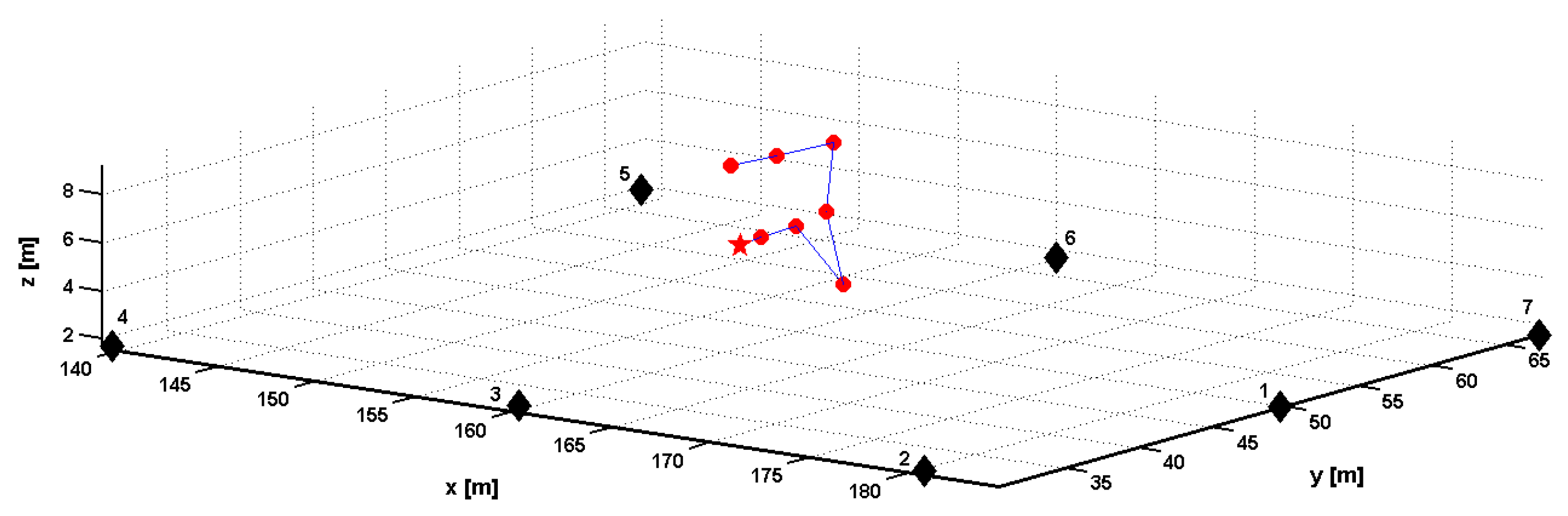
Simulations were conducted to investigate the performance of the proposed algorithms in order to better interpret the results of the real measurements. The performance of the algorithms was evaluated in terms of the root mean square error (RMSE) of the 3-D position estimates at a range of signal-to-noise ratio (SNR) levels. Details on the simulation setup and results are presented in Section 4.1 and 
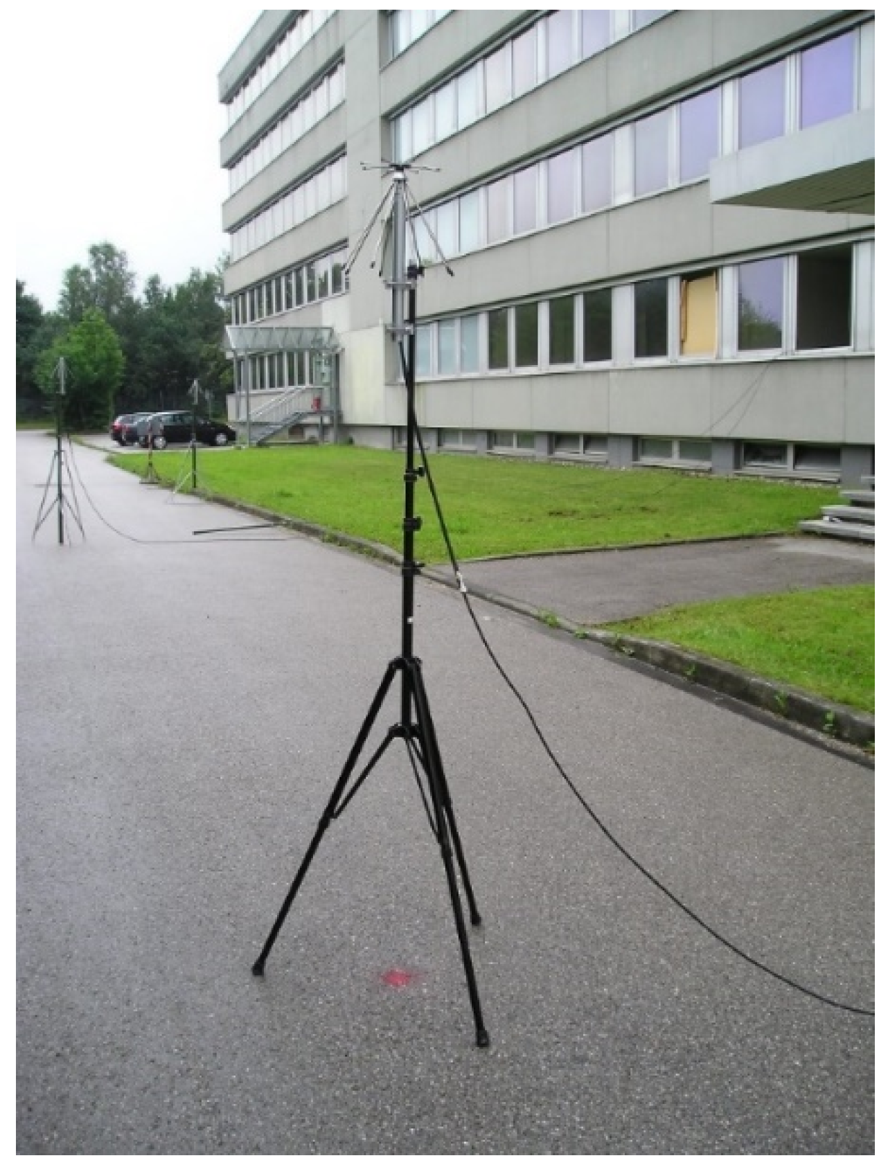
Section 4.2, respectively. To obtain real-world measurements, a wireless transmitter system was utilized to estimate the position of an indoor passive receiver using TDoA measurements. The system consists of a set of transmitting stations (TSs) located around the target building, user terminals (UTs) or receivers inside the building, and a monitoring and control unit (MCU) for steering the TSs and for broadcasting information to the UTs. TSs broadcast multicarrier navigation signals at 420 with 40 MHz bandwidth. The signal design allows minimizing multipath effects in harsh indoor environments, such as massive multilevel buildings made of concrete, steel, and metal-shielded windows. System architecture, details, and measurement examples are given in ref. [31] and references therein.
The following mathematical treatment is partially adopted from ref. [19] for convenience and is indicated by a citation before the equation. Consider an array of N transmitters located at known positions a i = [ x i , y i , z i ] T , in a 3-D Cartesian coordinate system, where i = 1, …, N and T is the transpose operator, and a passive receiver, at an unknown position a r = [ x r , y r , z r ] T , observing signals radiating from the transmitters. The receiver measures the TDoA of a pair of signals radiated by any pair of transmitters i and j, where i j . The TDoA measurement, τ i j , is related to the range difference, d i j , by the relation: d i j = c · τ i j , where c is the known propagation speed of the signal in the medium. Thus, d i j is expressed in the error-free case as [19]:
d i j = a j a r a i a r ,
where i = 1, …, N, j = 1, …, N, i j , and · denotes the Euclidean vector norm. The problem, thus, is to estimate the vector a r given a set of d i j , i.e., τ i j , noisy measurements and using the known vectors a i , which in turn might contain uncertainties.

3.1. Closed-Form Single Set Least Squares Solution

LSE makes no assumptions about the statistical characteristics of the measurement errors and therefore is an attractive alternative if the statistics of measurement errors cannot be determined accurately. Moreover, a CF estimator would be advantageous for practical real-time applications. The LSE minimizes a squared error function called the cost function. In the absence of measurement errors and transmitter position uncertainties, the LSE minimization will yield a zero-cost function. From Equation (1), we can get [19]:
a j a r 2 = [ d i j + a i a r ] 2 .
With straightforward algebra, Equation (2) yields [19]:
d i j · a i a r + [ a j a i ] T · a r = a j 2 a i 2 d i j 2 2 .
Without loss of generality, the first transmitter is considered as the master transmitter. Thus, Equation (3) is rewritten as [19]:
d 1 j · a 1 a r + [ a j a 1 ] T · a r = b 1 j ,
Where b 1 j = a j 2 a 1 2 d 1 j 2 2 and j = 2, …, N. The LSE would minimize a cost function, f c S S , which is expressed as [19]:
f c S S = j = 2 N ( d 1 j · a 1 a r + [ a j a 1 ] T · a r b 1 j ) 2 .
Equation (4) can be expressed in matrix form as H SS s SS = b SS , where [19]:
H SS = [ d 12 d 13 [ a 2 a 1 ] T [ a 3 a 1 ] T d 1 N [ a N a 1 ] T ] ,
b SS = [ b 12 b 13 b 1 N ] T ,
and:
s SS = [ a 1 a r a r ] .
Note that H SS is a ( N 1 ) × 4 matrix, b SS is a ( N 1 ) × 1 column vector, and s SS is a 4 × 1 column state vector, where the range a 1 a r to the master transmitter is a nuisance parameter. The cost function in Equation (5) can, thus, be rewritten using the matrix notation as f c S S = H SS s SS b SS 2 . The unconstrained CFSSLS solution of s SS reads [19]:
s ^ SS = ( H SS T H SS ) 1 H SS T b SS .
and the corresponding estimate of a r is given as [19]:
a ^ r = [ 0 1 1 1 ] s ^ SS .
We originally estimate the 4 × 1 state vector s SS . Therefore, we need at least four independent TDoA measurements with respect to a common master transmitter. That is, at least five transmitters are required in order to obtain a 3-D CF solution [19].
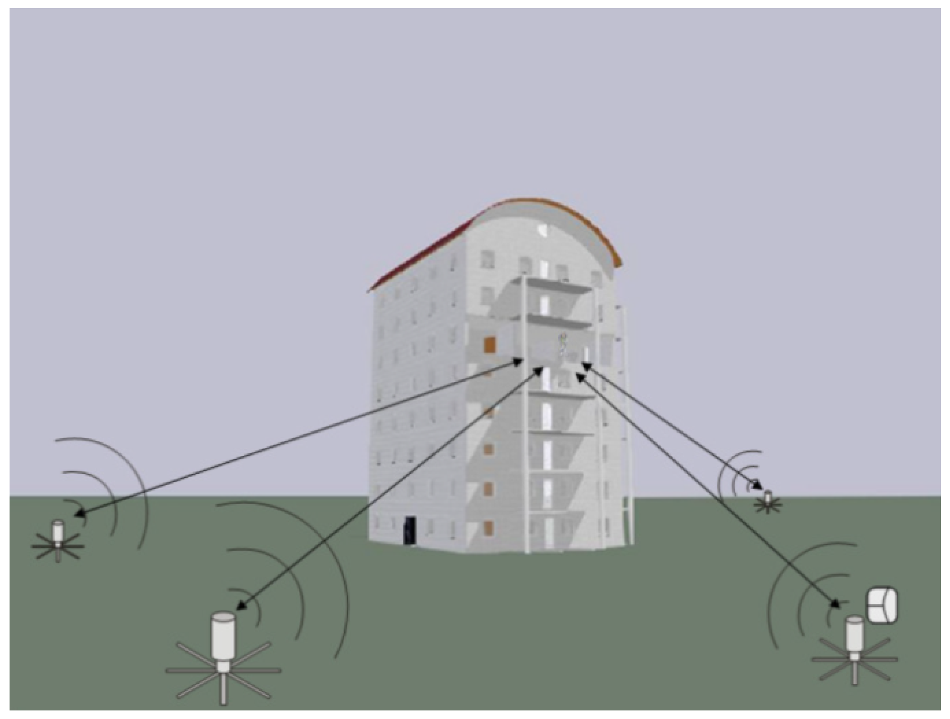
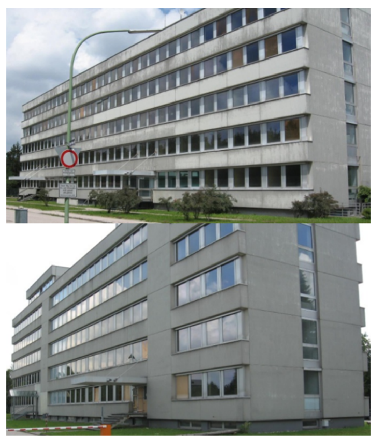
In a practical LPS, transmitters are often installed in coplanar or quasi-coplanar arrangements, see Figure 1. Such an arrangement is a major challenge for accurate 3-D positioning, namely, the vertical component of the 3-D position estimate is of poor accuracy, and therefore, the LPS would be useless for applications requiring accurate 3-D position estimates. The problem can be fixed by utilizing the nuisance parameter of the CFSSLS solution [20], which is the first element in the state vector, s SS , in Equation (8).
When coplanar or quasi-coplanar transmitters are used for TDoA measurements at the receiver, the CFSSLS solution of Equation (10) delivers acceptable accuracies for the 2-D, i.e., horizontal, position estimate, x ^ r , y ^ r , and poor estimates for the vertical position, z ^ r . Using the horizontal position estimate of the receiver, x ^ r , y ^ r , and the known horizontal coordinates of the first, i.e., master, transmitter, x 1 , y 1 
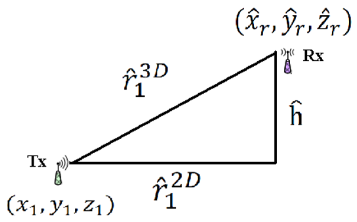
, the horizontal range from the receiver to the first (master) transmitter, r ^ 1 2 D , see Figure 2, can be estimated with acceptable accuracy as:
r ^ 1 2 D = ( x 1 x ^ r ) 2 + ( y 1 y ^ r ) 2 .
The 3-D range from the receiver to the master transmitter, a 1 a r , i.e., the nuisance parameter, which is the first element in the state vector, s SS , in Equation (8), is estimated by the CFSSLS algorithm as s ^ SS ( 1 ) and can be denoted as r ^ 1 3 D , see Figure 2. We can also see from Figure 2 that the difference, h = z r z 1 , between the vertical position of the receiver (Rx), z r , and the vertical position of the master transmitter (Tx), z 1 is estimated as:
h ^ = ( r ^ 1 3 D ) 2 ( r ^ 1 2 D ) 2 .
Thus, the estimate of the receiver’s vertical position, z ^ r , can be refined by:
z ^ r r e f i n e d = z 1 + α · h ^ ,
where α is a design parameter value, set by the system user, to adjust the amount of information obtained via Equation (12), i.e., the amount of information obtained by the utilization of the nuisance parameter. Thus, full information is included when α = 1 . When α = 0 , the vertical position of the receiver is set at the height of the master transmitter, i.e., nuisance parameter information is not included. The steps of the CFSSLS algorithm and the utilization of the nuisance parameter are exhibited in Algorithm 1.
Algorithm 1: The CFSSLS algorithm and refinement of the vertical position estimate.
0. Input: The known transmitters’ coordinates, i.e., a i = [ x i , y i , z i ] T , and the SS range difference measurements, i.e., d 1 j , as defined by Equation (4).
1. Compute: The matrix H SS and the vector b SS as defined by Equations (6) and (7), respectively.
2. Estimate: The state vector s SS by LS estimation via Equation (9).
3. CFSSLS Output: The receiver’s 3-D position estimate, i.e., a ^ r = [ x ^ r , y ^ r , z ^ r ] T , via Equation (10).
4. Estimate: The horizontal range, i.e., r ^ 1 2 D , from the receiver to the master transmitter via Equation (11).
5. Estimate: The difference, i.e., h ^ , between the vertical positions of the receiver and master transmitter via Equation (12).
6. Refine: The vertical position estimate of the receiver via Equation (13).
7. Output: The final 3-D position estimate of the receiver, i.e., a ^ r = [ x ^ r , y ^ r , z ^ r r e f i n e d ] T , where x ^ r , y ^ r were estimated in step 3 and z ^ r r e f i n e d was estimated in step 6.

3.2. Closed-Form Extended Single Set Least Squares Solution

The CF algorithm presented in ref. [18] is essentially based on transforming the hyperbolic equations into a set of vector equations by squaring the set of equations in Equation (1) and then differencing them. It requires a minimum of five transmitters, i.e., N = 5 , and uses an SS of the TDoA measurements in addition to extra measurements made by the successive pairs of the rest transmitters, so that the following ( N 1 ) + ( N 2 ) = 7 measurements are used: d 21 , d 31 , d 41 , d 51 , d 32 , d 43   and   d 54 . For an arbitrary number of transmitters, i.e., N 5 , the simultaneous equations are expressed in algebraic form, see ref. [18] for detailed derivation, as
a 11 · x r + a 12 · y r + a 13 · z r = b 1 a 21 · x r + a 22 · y r + a 23 · z r = b 2 a ( N 2 ) 1 · x r + a ( N 2 ) 2 · y r + a ( N 2 ) 3 · z r = b N 2
where:
a 11 = 2 d 21 ( x 2 x 1 ) 2 d 31 ( x 3 x 1 ) a 12 = 2 d 21 ( y 2 y 1 ) 2 d 31 ( y 3 y 1 ) a 13 = 2 d 21 ( z 2 z 1 ) 2 d 31 ( z 3 z 1 ) b 1 = 1 d 21 ( x 2 2 + y 2 2 + z 2 2 x 1 2 y 1 2 z 1 2 ) 1 d 31 ( x 3 2 + y 3 2 + z 3 2 x 1 2 y 1 2 z 1 2 ) + d 32
The other constants in the set of equations in Expression (14) can be similarly written as in Expression (15). Expression (14) can be put in the matrix form H ExSS s ExSS = b ExSS , where
H ExSS = [ a 11 a 12 a 13 a 21 a 22 a 23 a ( N 2 ) 1 a ( N 2 ) 2 a ( N 2 ) 3 ] ,
b ExSS = [ b 1 b 2 b N 2 ] T ,
and:
s ExSS = a r .
The dimension of the H ExSS matrix is ( N 2 ) × 3 , b ExSS is a ( N 2 ) × 1 column vector and s ExSS is a 3 × 1 column state vector. The matrix notation of the cost function to be minimized by the LSE is given by f c E x S S = H ExSS s ExSS b ExSS 2 . The unconstrained CF LS solution reads
a ^ r = ( H ExSS T H ExSS ) 1 H ExSS T b ExSS .
This is referred to as the CFExSSLS estimator. Note that only the unknown position vector of the receiver is estimated without any nuisance parameters. Therefore, this algorithm will deliver horizontal position estimates with acceptable accuracy and poor vertical position estimates if coplanar transmitters are used for 3-D positioning. The steps of the CFExSSLS solution are given in Algorithm 2.
Algorithm 2: The CFSSExLS algorithm.
0. Input: The known transmitters’ coordinates, i.e., a i = [ x i , y i , z i ] T , and the ExSS range difference measurements, i.e., d i 1 , d 32 , d 43 , ,   and   d N , N 1 .
1. Compute: The matrix H ExSS and the vector b ExSS as defined by Equations (16) and (17), respectively.
2. CFExSSLS Output: The receiver’s 3-D position estimate, i.e., a ^ r = [ x ^ r , y ^ r , z ^ r ] T , by the LS estimation in Equation (19).

3.3. Closed-Form Full Set Least Squares Solution

The set of measurement equations in the SS case is given in Equation (4). Accordingly, the set of measurement equations in the FS case can be straightforwardly written as [19]:
d 1 j · a 1 a r + [ a j a 1 ] T · a r = b 1 j , j = 2 , , N d 2 j · a 2 a r + [ a j a 2 ] T · a r = b 2 j , j = 3 , , N d N 1 , N · a N 1 a r + [ a N a N 1 ] T · a r = b N 1 , N ,
where also without loss of generality, the first, second, … and (N − 1)th transmitters are considered in order as reference transmitters, and the corresponding range difference measurements d i j = d j i are considered only once. Expression (20) can also be written in the matrix form H FS s FS = b FS , where [19]:
H FS = [ d 12 0 d 13 d 1 N 0 0 [ a 2 a 1 ] T 0 [ a 3 a 1 ] T 0 [ a N a 1 ] T 0 d 23 0 0 d 24 0 0 d 2 N 0 0 [ a 3 a 2 ] T 0 [ a 4 a 2 ] T 0 [ a N a 2 ] T 0 0 d N 1 , N [ a N a N 1 ] T ] ,
b F S = [ b 12 b 13 b 1 N b 23 b 24 b 2 N b N 1 , N ] T ,
and:
s F S = [ a 1 a r a 2 a r a N 1 a r a r ] T .
The H FS matrix has a dimension of N ( N 1 ) 2 × ( N + 2 ) , b FS is a N ( N 1 ) 2 × 1 column vector, and s FS is a ( N + 2 ) × 1 column state vector. The matrix notation of the cost function to be minimized by the LSE is given as f c F S = H FS s FS b FS 2 , and the unconstrained CFFSLS solution for s FS is written as:
s ^ FS = ( H FS T H FS ) 1 H FS T b FS .
Thus, the estimate of a r reads:
a ^ r = [ 0 0 1 1 1 ] s ^ FS .
Note that the number of nuisance parameters, i.e., a i a r , where i = 1 , , N 1 , in the ( N + 2 ) × 1 column state vector s FS given in Equation (23) increased to N 1 nuisance parameters, which are 3-D range estimates to the transmitters that were considered as master transmitters in the H FS matrix given in Equation (21), i.e., all transmitters with the indices 1 to N 1 [19].
The nuisance parameters can also be exploited to refine the vertical position estimate of the receiver using the TDoA measurements from coplanar or quasi-coplanar transmitters in a similar way to the procedure explained in Section 3.1 for the CFSSLS solution. Using the horizontal position estimate of the receiver, x ^ r , y ^ r , delivered by the CFFSLS solution, see Equations (24) and (25), and the known horizontal coordinates of the transmitters with the indices 1 to N 1 , i.e., x i , y i , where i = 1 , , N 1 , the horizontal ranges from the receiver to these transmitters, r ^ i 2 D , can be estimated with acceptable accuracy as:
r ^ i 2 D = ( x i x ^ r ) 2 + ( y i y ^ r ) 2 .
The 3-D ranges from the receiver to these transmitters, a i a r , i.e., the nuisance parameters, which are the first N 1 elements in the state vector, s FS , in Equation (23), are estimated by the CFFSLS algorithm as s ^ FS ( i ) , i = 1 , , N 1 and can be denoted as r ^ i 3 D . The differences, h i = z r z i , between the vertical position of the receiver, z r , and the vertical position of the transmitters, z i , are estimated as:
h ^ i = ( r ^ i 3 D ) 2 ( r ^ 1 2 D ) 2 .
We can determine the minimum vertical difference estimate, denoted as h ^ s e l e c t e d , from the difference estimates, h ^ i , according to:
h ^ s e l e c t e d = min i = 1 , , N 1 ( h ^ i ) .
Using h ^ s e l e c t e d and the vertical position of the corresponding transmitter, z s e l e c t e d , the estimate of the receiver’s vertical position, z ^ r , can be refined as:
z ^ r r e f i n e d = z s e l e c t e d + α · h ^ s e l e c t e d ,
where α is a design parameter value already defined. The steps of the CFFSLS algorithm and the utilization of the nuisance parameters are listed in Algorithm 3.
Algorithm 3: The CFFSLS algorithm and refinement of the vertical position estimate.
0. Input: The known transmitters’ coordinates, i.e., a i = [ x i , y i , z i ] T , and the FS range difference measurements, i.e., d 1 j , d 2 j , ,   and   d N 1 , N , as defined by the set of equations in (20).
1. Compute: The matrix H FS and the vector b FS as defined by Equations (21) and (22), respectively.
2. Estimate: The state vector s FS by LS estimation via Equation (24).
3. CFFSLS Output: The receiver’s 3-D position estimate, i.e., a ^ r = [ x ^ r , y ^ r , z ^ r ] T , via Equation (25).
4. Estimate: The horizontal ranges, i.e., r ^ i 2 D , from the receiver to the transmitters i = 1 , , N 1 via Equation (26).
5. Estimate: The differences, i.e., h ^ i , between the vertical positions of the receiver and transmitters i = 1 , , N 1 via Equation (27).
6. Find: The minimum vertical difference estimate, i.e., h ^ s e l e c t e d , via Equation (28).
7. Refine: The vertical position estimate of the receiver via Equation (29).
8. Output: The final 3-D position estimate of the receiver, i.e., a ^ r = [ x ^ r , y ^ r , z ^ r r e f i n e d ] T , where x ^ r , y ^ r were estimate in step 3 and z ^ r r e f i n e d was estimated in step 7.

4. Results

4.1. Simulation Setup

Computer simulations were conducted using MATLAB to evaluate the performance of the proposed TDoA-based CF LS algorithms in terms of the RMSE at a range of SNR levels from −5 to 40 dB. The range difference measurement was simulated as true value, d i j , where i j , added with error. The error has two components: A constant bias (positive or negative), b, and a zero-mean Gaussian noise. The SNR of any range difference signal is defined as [32]:
S N R = 10 l o g d i j 2 σ i 2   [ dB ] .
Thus, the variance of the Gaussian noise, σ i 2 , is computed as [32]:
σ i 2 = d i j 2 10 S N R / 10 .
The constant bias is defined as:
b = ± 0.1 · d i j 2 .
A seven-transmitter geometry, listed in Table 1, was considered to resemble the experimental transmitters’ geometrical arrangement in order to get representative simulation results. The receiver was placed at 160, 50, and 6 m. The layout of the receiver and transmitters is shown in Figure 3.
Five error input conditions were considered: noise only, positive bias only, noise plus positive bias, negative bias only, and noise plus negative bias. The statistical result of 10,000 independent runs in each error input condition was considered for the RMSE performance, except in the bias only error input conditions, where only a single simulation run was necessary since the bias was constant over the range of considered SNR levels, and therefore, the root square error (RSE) of the position estimate is obtained. The RMSE performance was separated into the horizontal, i.e., xy, and the vertical, i.e., z, spaces, and were, respectively, defined as:
x y   R M S E = 1 n i = 1 n [ ( x r x ^ r i ) 2 + ( y r y ^ r i ) 2 ]
and:
z   R M S E = 1 n i = 1 n [ ( z r z ^ r i ) 2 ] ,
where n is the number of simulation runs. Thus, the overall 3-D RMSE, i.e., xyz RMSE, is defined as:
x y z   R M S E = 1 n i = 1 n [ ( x r x ^ r i ) 2 + ( y r y ^ r i ) 2 + ( z r z ^ r i ) 2 ] .

4.2. Simulation Results

4.2.1. Noise Only Results

Figure 4 plots the xy RMSE of the CFSSLS, CFExSSLS, and CFFSLS solutions versus the SNR. We see that the CFSSLS algorithm performed best followed by the CFExSSLS algorithm at high SNR levels. The CFSSLS algorithm utilizes only the independent measurements, i.e., all noises appear just once, unlike the CFExSSLS algorithm that also utilizes some dependent measurements, and therefore, some noises affect more than once and increase the overall estimation error. The CFFSLS algorithm performance seems to be insensitive to noise, as shown by its almost constant accuracy over the range of SNR levels. Here, noises affect several times, positively and negatively, through propagation into the extra dependent measurements utilized in the algorithm. The performance of the CFExSSLS algorithm deteriorates rapidly below the 10 dB SNR level, while the CFSSLS solution accuracy starts to decrease below the 5 dB SNR level. At very high noise levels, below 5 dB, the CFFSLS algorithm delivers the best possible solution. The insensitivity of the CFFSLS solution to noise indicates the upper bound on the horizontal position accuracy attainable at high noise levels, which is the case in environments that are challenging to wireless signals. Figure 5 shows a similar trend in the vertical space. However, the vertical position estimates of the three algorithms in their original formulation are useless due to the quasi-coplanar arrangement of the involved transmitters; thus, only the horizontal position estimates can be accepted.
Figure 6 shows the z RMSE of the CFSSLS and CFFSLS algorithms when the nuisance parameters are utilized to refine the vertical position estimates as explained in Section 3.1 and Section 3.3. The CFExSSLS solution does not estimate any nuisance parameters to be utilized in a similar procedure. The accuracy of the vertical position estimates was reduced to a couple of meters. The accuracy of the CFSSLS refined solution ranged between about 2.10 and 3.35 m, and that of the CFFSLS refined solution between 1.50 and 2.50 m. The better accuracy was generally obtained at lower SNR levels, especially for the CFSSLS solution, while the less accurate estimates of the CFFSLS solution were obtained in the 10 to 20 dB SNR levels. The accuracy of the CFFSLS solution decreases slightly after 0 dB to reach less than 2.5 m at 15 dB and then starts again to increase to an almost constant accuracy of less than 2 m at SNR ≥ 30 dB. Both algorithms deliver similar accuracies between about 8 and 15 dB. However, the accuracy differences over the range of SNR levels are still not greatly significant, they are less than 1.5 and 1 m for the CFSSLS and CFFSLS solutions, respectively, and depend on the geometry of receiver and transmitters. The CFFSLS algorithm delivered more accurate refined vertical position estimates due to the utilization of more nuisance parameters, which is equivalent to the utilization of more information.

4.2.2. Positive Bias Only Results

From Figure 7, we see that in the case of positive bias only measurement errors, the CFSSLS algorithm delivers the most accurate horizontal position estimate. This result is consistent since all biases contribute to the CFSSLS solution only once, unlike the CFExSSLS and CFFSLS solutions, where bias errors contribute more than once due to the utilization of extra dependent measurements beyond the SS independent set of TDoA measurements. It would further be expected that the horizontal positioning accuracy of the CFExSSLS solution has to be higher than that of the CFFSLS solution, since it utilizes fewer dependent measurements. However, as can be seen from Figure 7, the horizontal positioning accuracy of both the CFExSSLS and CFFSLS algorithms are identical, indicating the canceling-out of some bias effects when using the FS of TDoA measurements, resulting in the identical horizontal accuracy of the CFExSSLS and CFFSLS solutions. A similar and more obvious trend for the vertical positioning accuracy is seen from Figure 8, despite the fact that these vertical position estimates are useless due to the quasi-coplanar arrangement of the transmitters. The most accurate vertical position estimate is obtained by the CFSSLS algorithm followed by the CFExSSLS algorithm and then by the CFFSLS algorithm. No canceling-out of bias errors in the FS TDoA equations obviously appeared in the vertical, i.e., one-dimensional, space. Figure 9 confirms again that the accuracy of the CFFSLS refined vertical position estimate is higher than that of the CFSSLS result, since more nuisance parameters are utilized by the CFFSLS algorithm to refine the vertical position estimate. The accuracies of the CFFSLS and CFSSLS refined vertical position estimates are 0.30 and less than 1.10 m, respectively.

4.2.3. Noise Plus Positive Bias Results

Figure 10 plots the xy RMSE of the CFSSLS, CFExSSLS, and CFFSLS solutions when simulated measurements are corrupted by noise and positive bias. At high SNR levels, the best performance is obtained by the CFSSLS algorithm, as expected, and both the CFExSSLS and CFFSLS solutions are identical, in accordance with the results from Figure 7, as long as measurement errors are dominated by positive bias. The CFFSLS solution is almost insensitive to the noise level and outperforms the CFSSLS solution at high noise levels, i.e., below 5 dB. The z RMSE trend, shown in Figure 11, is similar to that in the noise-only case plotted in Figure 5. At high SNR levels, the CFSSLS algorithm performs best and is followed by the CFExSSLS algorithm. As the noise level increases, the CFFSLS solution outperforms the CFExSSLS and CFSSLS below 15 and 5 dB, respectively. We repeat again that all these vertical position estimates are useless for 3-D applications due to the quasi-coplanar arrangement of the transmitters. The z RMSE of the refined vertical position estimates of the CFSSLS and CFFSLS algorithms are plotted in Figure 12. The CFFSLS solution outperforms the CFSSLS solution due to the utilization of more nuisance parameters. The vertical position estimates are accurate enough for many 3-D applications.

4.2.4. Negative Bias Only Results

From Figure 13, we see that the CFExSSLS algorithm performs much better than the CFFSLS algorithm and approaches the performance of the CFSSLS solution in horizontal space, xy, unlike with positive bias only errors, see Figure 7, in which the CFExSSLS estimation approaches towards the CFFSLS solution, where both have identical performance. Figure 14 shows that the vertical positioning performance of the CFExSSLS algorithm is better than the other two solutions. When comparing Figure 13 with Figure 7 and Figure 14 with Figure 8, it seems that negative bias errors enhance the horizontal and vertical positioning performance of the CFExSSLS algorithm, while the relative performances of the CFSSLS and CFFSLS algorithms are not greatly affected. Figure 15 shows that the accuracy of the CFSSLS refined vertical position estimation is slightly better than that of the CFFSLS solution, i.e., it reverses the result in Figure 9, which indicates that negative bias errors degrade the advantage of using more nuisance parameters.

4.2.5. Noise Plus Negative Bias Results

Figure 16 plots the xy RMSE of the CFSSLS, CFExSSLS, and CFFSLS solutions when simulated measurements are corrupted by noise and negative bias. At high SNR levels, the best performance is obtained by the CFSSLS algorithm and the CFExSSLS solution approaches the CFSSLS solution very tightly when measurement errors are dominated by negative bias, which is a result obtained in the previous subsection, see Figure 13. The constant performance of the CFFSLS algorithm outperforms the CFExSSLS and CFFSLS solutions below the 15 and 5 dB SNR levels, respectively. The z RMSE performance in Figure 17, despite its uselessness for 3-D positioning, shows that at high SNR levels, the CFExSSLS algorithm performs better than the other two solutions, a result obtained from Figure 14. The performances of the CFExSSLS and CFSSLS solutions deteriorate further also below the 15 and 5 dB SNR levels, respectively. The z RMSE of refined vertical position estimates of the CFSSLS and CFFSLS algorithms are always below 2.5 m as depicted in Figure 18.

4.3. Experimental Setup and Results

Real-world TDoA measurements were obtained in a multilevel massive building of 66.25 m length and 11.94 m width, see Figure 19. The test building is made of 60 cm thick reinforced concrete with metal shielded windows. Seven transmitters were installed outside the building, see Figure 20, and a test receiver indoors observed the TDoA of the transmitted signal at eight reference test positions. The layout of the receiver test positions and the transmitters is illustrated in Figure 21. The coordinates of the transmitters and the test receiver positions are listed in Table 1 and Table 2, respectively. Table 2 also includes the number of TDoA measurement epochs (runs) at each receiver test position. This total NLoS situation and the material properties of the test building are extremely challenging to wireless signals when used for positioning. NLoS bias errors and high-level noise are expected in this experimental scenario. Figure 22 shows the error of the SS range difference measurements at the eight receiver test positions, and Figure 23 illustrates the histograms of these measurement errors. From both figures, we can see that the measurement errors are a mix of positive and negative biases added to non-uniform noises and some outliers. The mean errors of these SS measurements at the test positions are listed in Table 3.
Table 4 lists the RMSE of the horizontal, vertical, and overall 3-D positioning performance of the CFSSLS, CFExSSLS, and CFFSLS algorithms. The horizontal positioning accuracies of the CFSSLS, CFExSSLS, and CFFSLS solutions were, respectively, 3.57, 2.91, and 2.90 m. As mentioned before, the vertical position estimates without refinement are useless. The refined vertical positioning of both the CFSSLS and CFFSLS solution were similar, i.e., 2.59 and 2.61 m, respectively. Thus, the overall 3-D positioning accuracy of the CFFSLS algorithm, i.e., 3.90 m, is higher than the accuracy of the CFSSLS algorithm, i.e., 4.41 m, during the experiments, in which total NLoS conditions and low SNR levels prevailed.

5. Discussion

There are no positioning algorithms that best fit in all environments, situations, and wireless signal conditions. Positioning algorithms are usually developed for certain special cases because real environments are complex, and the geometries of receivers and transmitters are quite variable [11]. Despite improvements in wireless, hardware, and software technologies, the development of low-cost and high-accuracy positioning systems is still a challenging task. Therefore, new positioning systems and approaches will be developed in the next few years since the current technology has not yet matured.
The experimental testing and evaluation of any indoor positioning system is a difficult task due to the need for a network deployment and for testing in several types of buildings [33]. If a particular system is intended to be widely deployed, specific testing and evaluation in expected deployment environments may make sense. However, the repeatability of tests in the same environment is difficult to achieve because it is almost impossible to repeat the same environmental and signal conditions. Therefore, measures should be developed in order to create almost constant testing and evaluation conditions, in order to maximize repeatability and enable objective and fair performance comparisons. Repeatability can easily be achieved by simulations. However, simulation may not always be able to exactly resemble the varying conditions of the real world.
As previously indicated in ref. [19], the TDoA-based positioning technique has increasing practical and theoretical importance in a wide range of applications. The TDoA measurements used in CF parametric estimation also depend on some nuisance parameters. The question of whether it is advantageous to exploit the knowledge about the nuisance parameters was addressed. Knowledge about the nuisance parameters is equivalent to having a more precise probabilistic model [34] for the stochastic connection between the TDoA measurements and the receiver’s position. Thus, it contributes to uncertainty and estimation error reduction. The optimal exploitation of the knowledge about nuisance parameters or the contribution of this knowledge to theoretical lower bounds, e.g., the Cramer–Rao lower bound (CRLB), on the estimation errors are issues that still need further research efforts [19]. The system designer often wants to know in advance the best an estimator can perform as a check against available designs in certain situations. The CRLB provides a benchmark for the best positioning accuracy for any unbiased estimator, e.g., the CFSSLS estimator. Both the CFExSSLS and CFFSLS are biased estimators since they use dependent TDoA measurements. If perfect knowledge of the real world is available, the CFSSLS estimator can deliver the best performance. However, an estimator designed to approach the CRLB is not robust if the estimator is not perfectly matched to the real world. The CRLB provides no indication of what to do to achieve the predicted performance in the presence of uncertainty. Therefore, the practical meaning of the CRLB is no other than to say that the designer must have perfect knowledge about the real world to obtain small estimation errors. Investigating the performance of estimators given some level of uncertainty yields the best an estimator can do. In this regard, a CRLB lacks a practical meaning, because it assumes that even smaller errors can be achieved, but without providing any indications of how to attain the predicted performance given the present level of uncertainty. Therefore, the CRLB might not always represent an objective to achieve when designing a practical estimator.
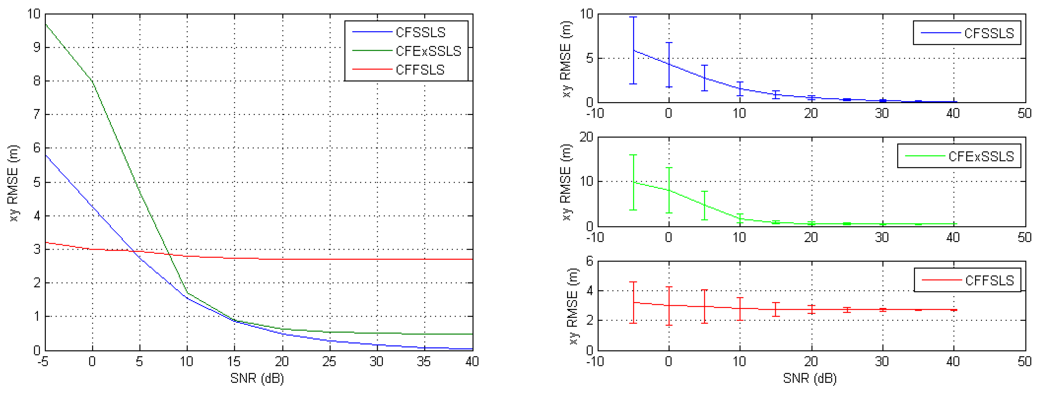
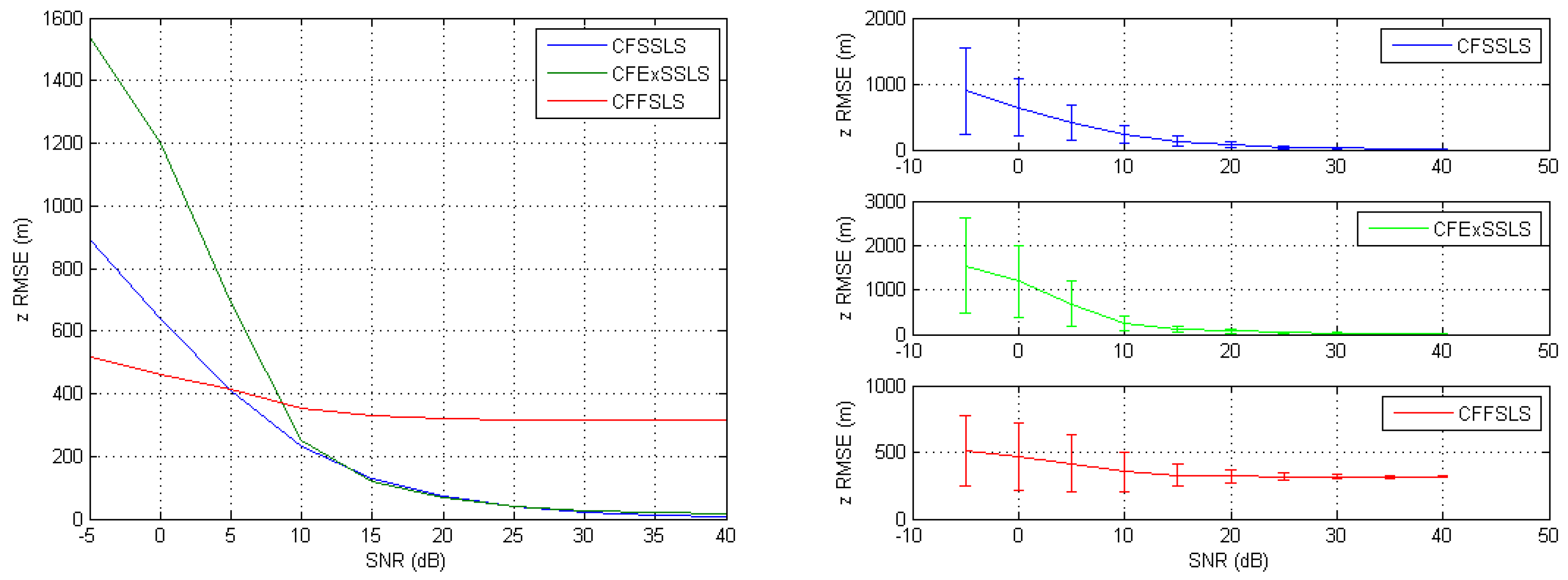
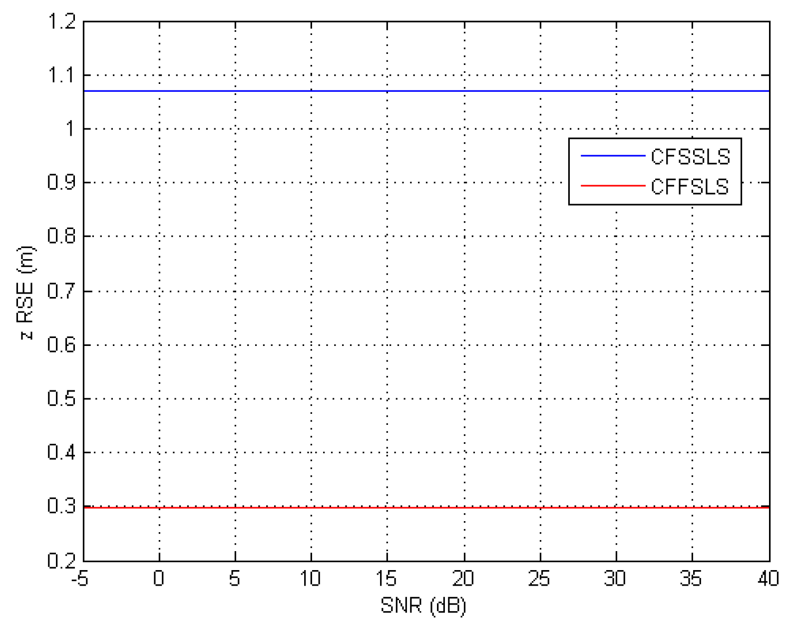
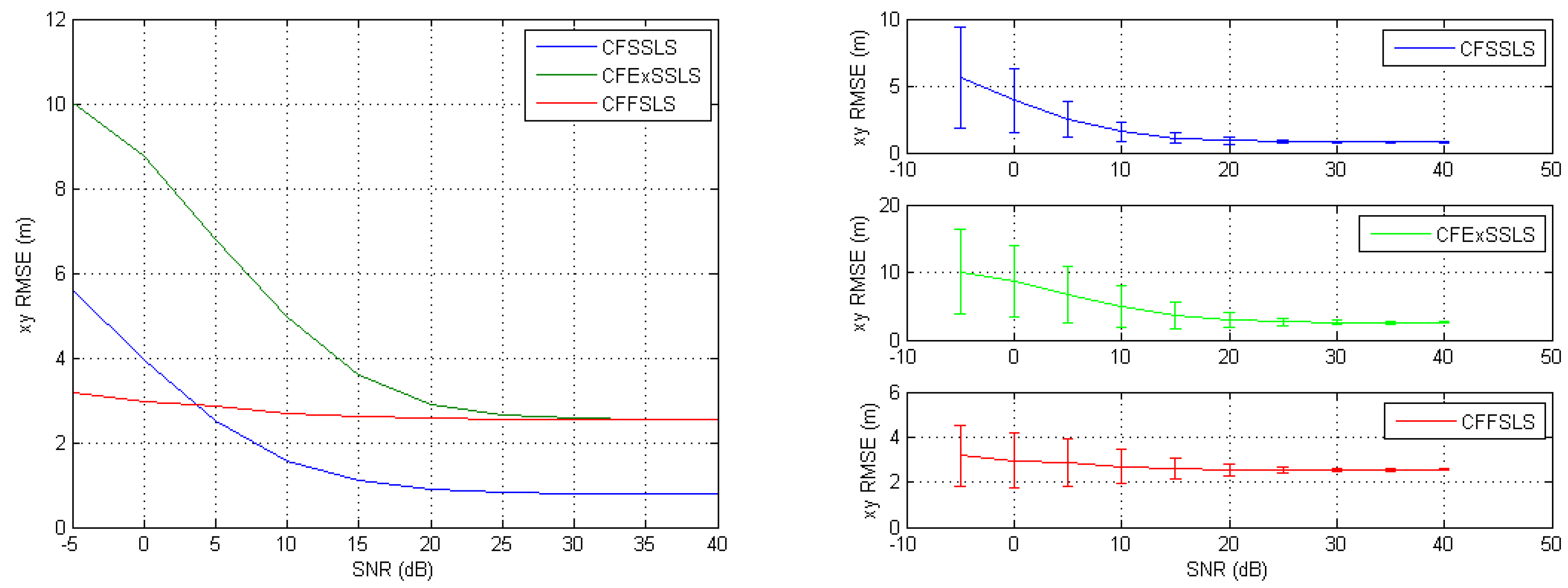
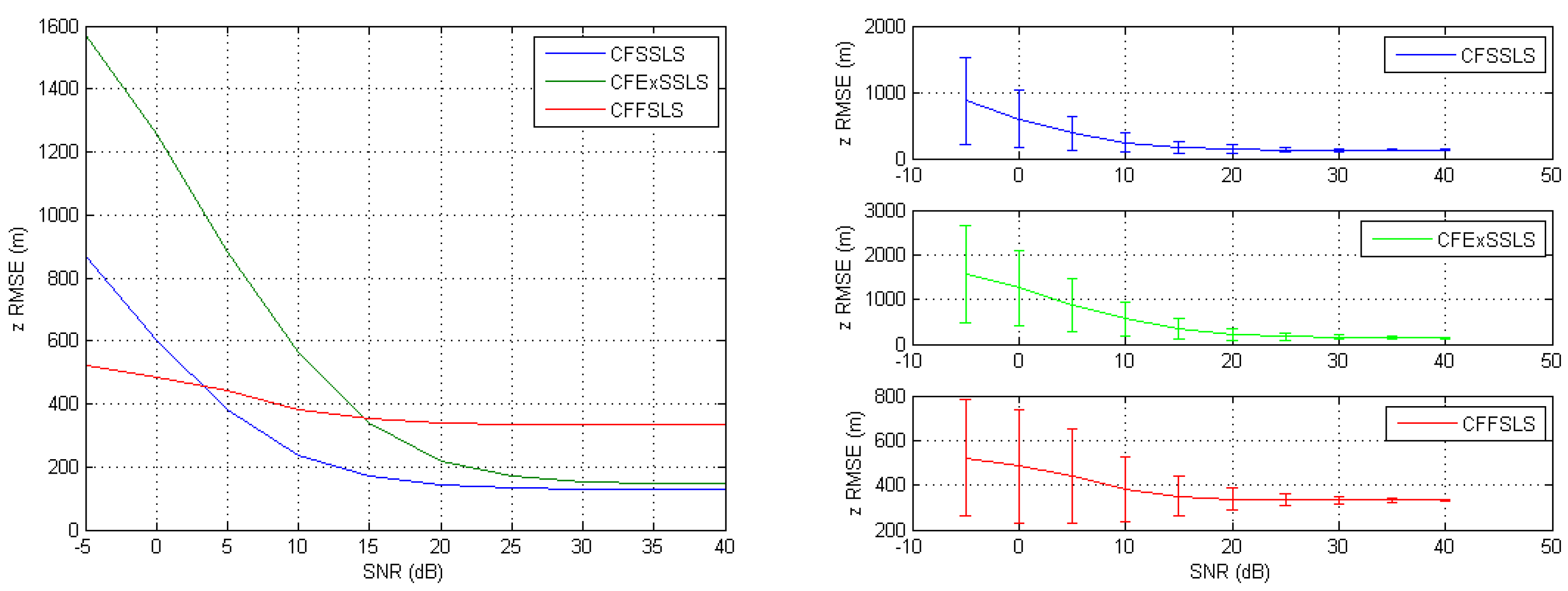
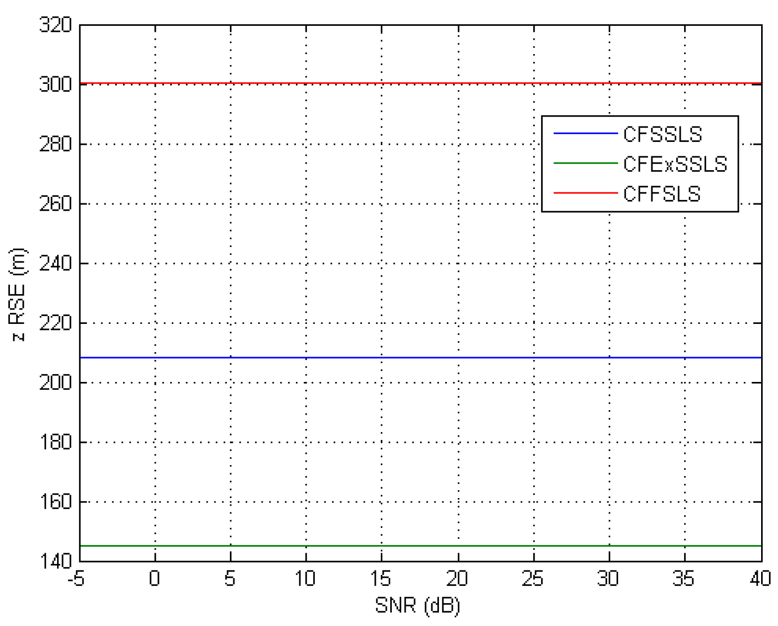
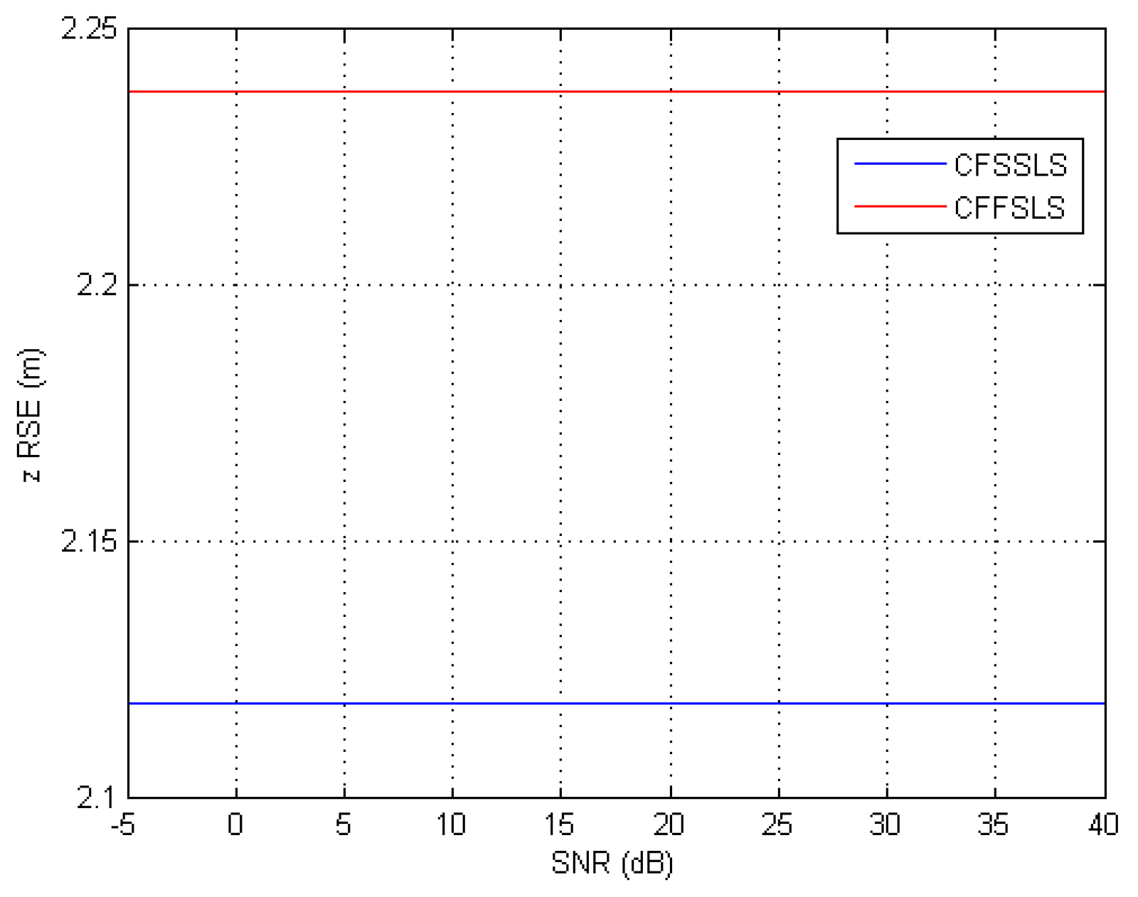
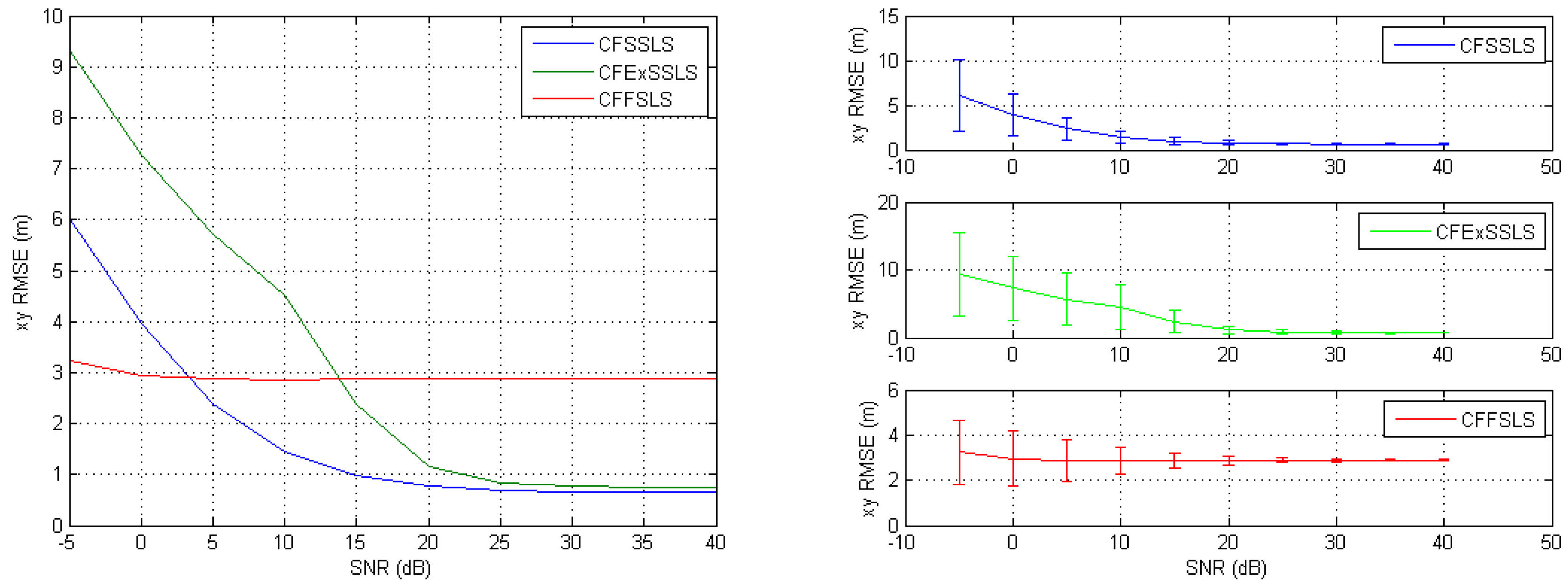
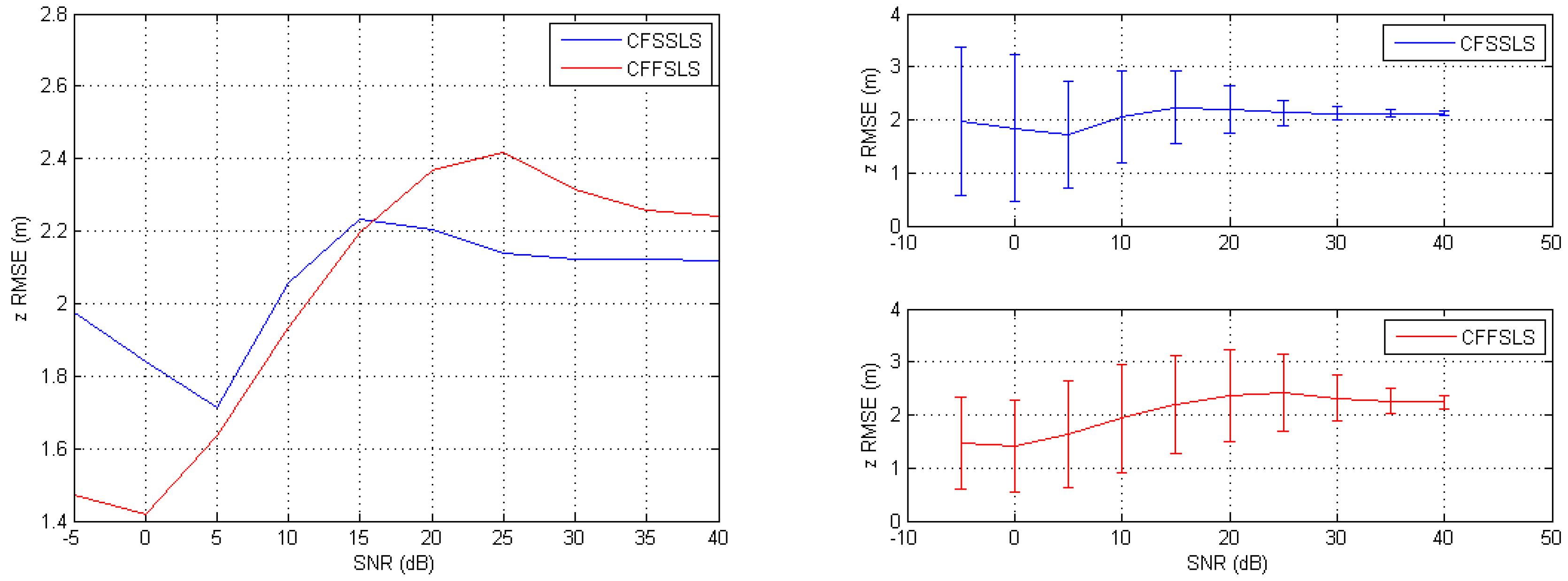
When simulated TDoA measurements were only corrupted by noise, the best position estimates were obtained by the CFSSLS, CFExSSLS, and CFFSLS solutions (ordered from best to worst), respectively, at moderate to high SNR levels. At low SNR levels, i.e., high noise levels, the CFFSLS algorithm delivers the best estimates. The CFFSLS algorithm is a biased solution, where noises contribute many times in different combinations leading to cancel-out effects, which are indicated by the constant accuracy, i.e., steady-state behavior, over the range of investigated SNR levels. The CFSSLS and CFFSLS algorithms can refine the vertical position estimate if they utilize the nuisance parameters. Generally, the CFFSLS solution delivers more accurate refined vertical position estimates as it utilizes more nuisance parameters, i.e., more information, than the CFSSLS solution.
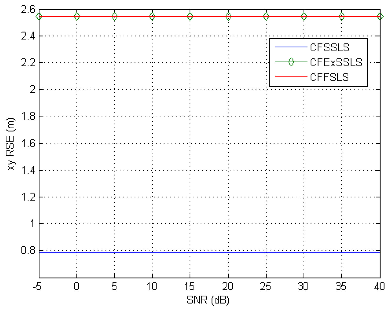
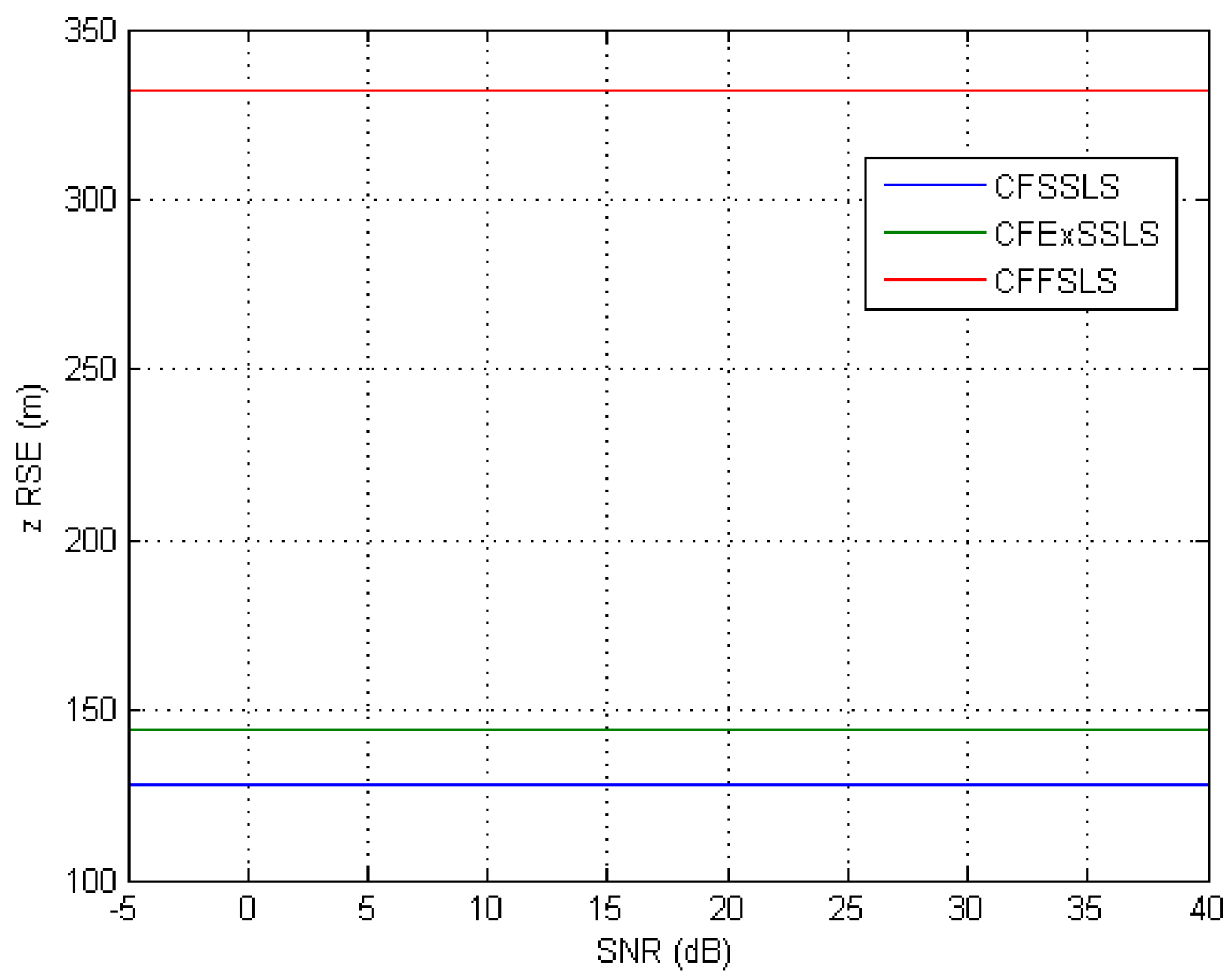
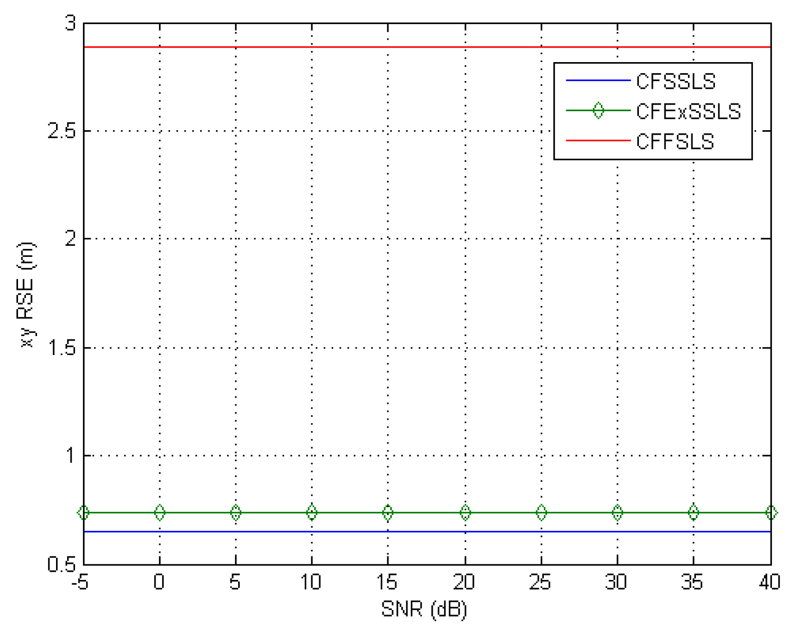
When only positive bias errors were present in the simulated TDoA measurements, the most accurate position estimates were obtained by the CFSSLS, CFExSSLS, and CFFSLS solutions (ordered from more to less accurate), respectively. In the horizontal space, using the FS TDoA measurements cancels out some bias effects and renders the CFExSSLS and CFFSLS solutions identical. The refined vertical position estimate of the CFFSLS algorithm is more accurate than that of the CFSSLS algorithm due to the utilization of more nuisance parameters.
The results of the two error input conditions, noise only and positive bias only, were consistently combined when simulated TDoA measurement errors were corrupted by noise and positive bias. The best performance is obtained by the CFSSLS algorithm followed by the CFExSSLS algorithm and then by the CFFSLS algorithm at moderate to high SNR levels. Both the CFExSSLS and CFFSLS horizontal position estimates are identical at high SNR levels. The CFFSLS solution is insensitive to the SNR level and, therefore, outperforms the other two solutions at low SNR, i.e., high noise, levels. The refined vertical position estimates of the CFFSLS solution is more accurate due to the utilization of more nuisance parameters.
The simulations showed that negative bias only errors generally favored the CFExSSLS algorithm more than the other two solutions. In the horizontal space, the CFSSLS algorithm performed best and closely followed by the CFExSS solution. In the vertical space, the CFExSSLS algorithm was less affected than the other two algorithms. Negative biases also did not favor the utilization of more nuisance parameters for refining the vertical position estimation. The accuracy of the CFSSLS refined vertical position estimation is slightly better than that of the CFFSLS solution. Similar conclusions also apply when noise is added to negative bias errors.
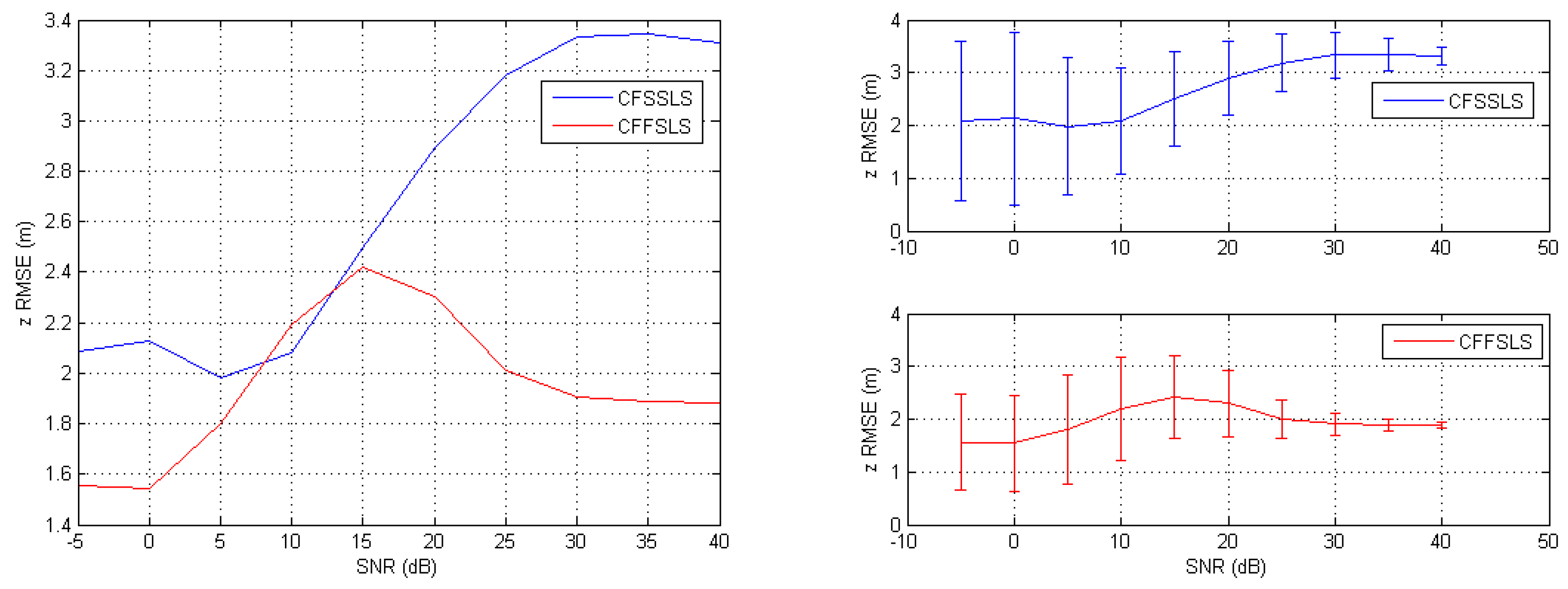
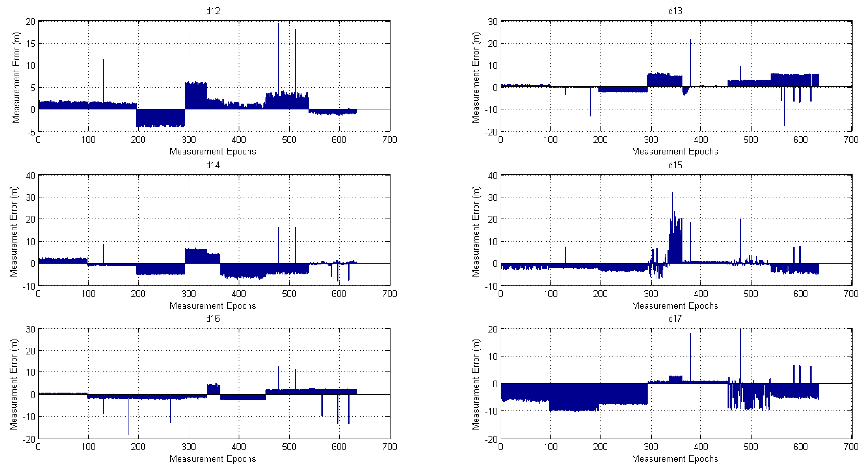
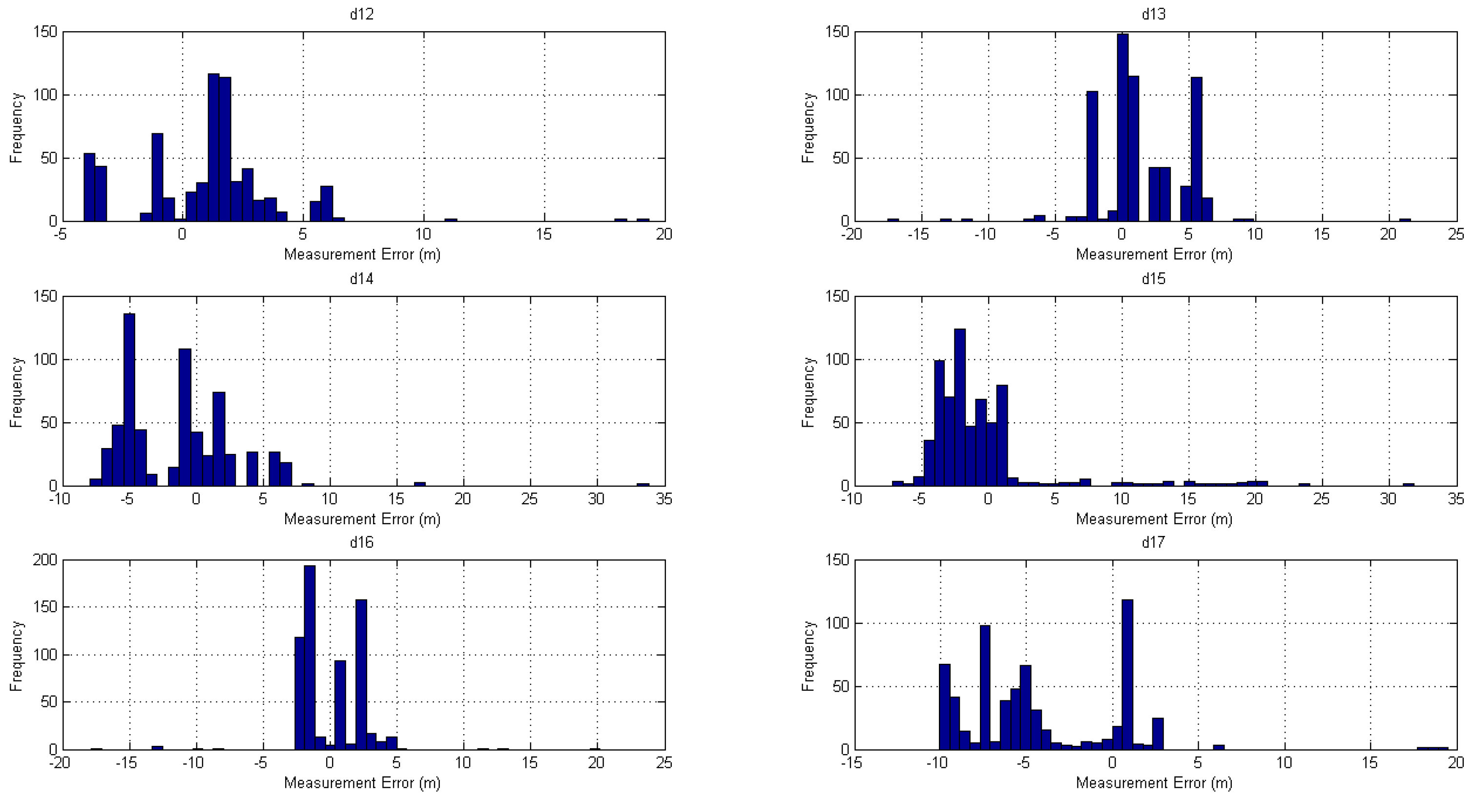
The experimental measurement errors contained a mix of the error conditions studied in the simulations. The CFFSLS algorithm had a better performance in the RMSE sense, since total NLoS conditions and non-uniform SNR levels prevailed during the experiments.
Thus, the concept of obtaining useful receiver’s vertical position estimates by the utilization of nuisance parameters in the coplanar transmitters’ setting was proved. However, a comprehensive evaluation of the approach is still needed, by repeating the experiments many times on different days and in several test buildings with different characteristics, in order to meet the recommendations provided in ref. [33].

6. Conclusions

It was demonstrated with simulations and experiments that with quasi-coplanar arrangement of transmitters and at moderate to high SNR levels, the CFSSLS solution had the best performance, followed by the CFExSSLS solution and then by the CFFSLS solution. At low SNR levels, the CFFSLS algorithm outperformed the other two algorithms. Both the CFSSLS and CFFSLS solutions estimate nuisance parameters. It was also demonstrated that the exploitation of these parameters was useful, in accordance with intuition, to significantly increase, i.e., refine, the accuracy of the receiver’s vertical position estimates. This study invites for more specific investigations to test and evaluate the presented approaches for potential positioning applications, in order to demonstrate that more conclusive results may be found for certain sets of error conditions, since different sets of error conditions seem to favor one algorithm over the other. Therefore, more research is needed to further develop and test the proposed ideas in a wider range of environments and error conditions.

Funding

This research received no external funding.

Acknowledgments

Open Access Funding by the Publication Fund of the TU Dresden.

Conflicts of Interest

The author declares no conflict of interest.

Abbreviations

AoAAngle of Arrival
CFClosed-Form
CFExSSLSClosed-Form Extended Single Set Least Squares
CFFSLSClosed-Form Full Set Least Squares
CFSSLSClosed-Form Single Set Least Squares
CRLBCramer–Rao Lower Bound
DMDirect Method
DPDDirect Position Determination
ExSSExtended Single Set
FSFull Set
GNSSGlobal Navigation Satellite System
LCLSLinear Correction Least Squares
LoSLine-of-Sight
LPSLocal Positioning Systems
LSLeast Squares
LSELeast Squares Estimation or Estimator
MCUMonitoring and Control Unit
MLMaximum Likelihood
MLEMaximum Likelihood Estimator
NLoSNon-Line-of-Sight
PDoAPhase Difference of Arrival
PoAPhase of Arrival
RFRadio Frequency
RMSERoot Mean Square Error
RSERoot Square Error
RSSReceived Signal Strength
RToFRound-Trip Time of Flight
SISpherical Interpolation
SNRSignal-To-Noise Ratio
SSSingle Set
ToATime of Arrival
TDoATime Difference of Arrival
TSTransmitting Station
UTUser Terminal

References

  1. Dargie, W.; Poellabauer, C. Fundamentals of Wireless Sensor Networks: Theory and Practice; John Wiley & Sons: New York, NY, USA, 2010. [Google Scholar]
  2. Zafari, F.; Gkelias, A.; Leung, K. A Survey of Indoor Localization Systems and Technologies. arXiv 2019, arXiv:1709.01015v3. [Google Scholar] [CrossRef] [Green Version]
  3. Kelner, J.M.; Ziolkowski, C.; Nowosielski, L.; Wnuk, M.T. Localization of emission source in urban environment based on the Doppler effect. In Proceedings of the 2016 IEEE 83rd Vehicular Technology Conference (VTC Spring), Nanjing, China, 15–18 May 2016; pp. 1–5. [Google Scholar]
  4. Gajewski, P.; Ziółkowski, C.; Kelner, J.M. Using SDF method for simultaneous location of multiple radio transmitters. In Proceedings of the 19th International Conference on Microwaves, Radar & Wireless Communications (MIKON-2012), Warsaw, Poland, 21–223 May 2012; Volume 2, pp. 634–637. [Google Scholar]
  5. Amar, A.; Weiss, A.J. Localization of narrowband radio emitters based on Doppler frequency shifts. IEEE Trans. Signal Process. 2008, 56, 5500–5508. [Google Scholar] [CrossRef]
  6. Yang, Z.; Zhou, Z.; Liu, Y. From RSSI to CSI: Indoor localization via channel response. ACM Comput. Surv. 2013, 46, 25. [Google Scholar] [CrossRef]
  7. Xiong, J.; Jamieson, K. ArrayTrack: A fine-grained indoor location system. In Proceedings of the 10th USENIX Symposium on Networked Systems Design and Implementation (NSDI 13), Lombard, IL, USA, 2–5 April 2013; pp. 71–84. [Google Scholar]
  8. Amar, A.; Weiss, A.J. Direct position determination in the presence of model errors—Known waveforms. Digit. Signal Process. 2006, 16, 52–83. [Google Scholar] [CrossRef]
  9. Qin, T.; Li, L.; Ba, B.; Wang, D. A fast ML-based single-step localization method using EM algorithm based on time delay and Doppler shift for a far-field scenario. Sensors 2018, 18, 4139. [Google Scholar] [CrossRef] [PubMed] [Green Version]
  10. Tzoreff, E.; Weiss, A.J. Expectation-maximization algorithm for direct position determination. Signal Process. 2017, 133, 32–39. [Google Scholar] [CrossRef]
  11. Li, X.; Deng, Z.D.; Rauchenstein, L.T.; Carlson, T.J. Contributed Review: Source-localization algorithms and applications using time of arrival and time difference of arrival measurements. Rev. Sci. Instrum. 2016, 87, 921–960. [Google Scholar] [CrossRef]
  12. Foy, W. Position-location solutions by Taylor-series estimation. IEEE Trans. Aerosp. Electron. Syst. 1976, 12, 187–194. [Google Scholar] [CrossRef]
  13. Torrieri, D. Statistical theory of passive location systems. IEEE Trans. Aerosp. Electron. Syst. 1984, 20, 183–197. [Google Scholar] [CrossRef] [Green Version]
  14. Fletcher, R.; Powell, M. A rapidly convergent descent method for minimization. Comput. J. 1963, 6, 163–168. [Google Scholar] [CrossRef]
  15. Marquardt, D. Algorithm for least-squares estimation of nonlinear parameters. SIAM J. Appl. Math. 1963, 11, 431–441. [Google Scholar] [CrossRef]
  16. Chen, J.; Hudson, R.; Yao, K. Maximum-likelihood source localization at unknown sensor location estimation for wideband signals in the near-field. IEEE Trans. Signal Process. 2002, 50, 1843–1854. [Google Scholar] [CrossRef]
  17. Stoica, P.; Li, J. Source localization from range-difference measurements. IEEE Signal Process. Mag. 2006, 23, 63–65. [Google Scholar] [CrossRef]
  18. Bakhoum, E. Closed-Form Solution of Hyperbolic Geolocation Equations. IEEE Trans. Aerosp. Electron. Syst. 2006, 42, 1396–1404. [Google Scholar] [CrossRef]
  19. Khalaf-Allah, M. An extended closed-form least-squares solution for three-dimensional hyperbolic geolocation. In Proceedings of the 2014 IEEE Symposium on Industrial Electronics Applications (ISIEA), Kota Kinabalu, Malaysia, 28 September–1 October 2014; pp. 7–11. [Google Scholar]
  20. Khalaf-Allah, M.; Qaisar, S.U. Nuisance Parameter Exploitation for Accurate 3D Hyperbolic Geolocation—Field Results. In Proceedings of the International Radar Symposium (IRS-2013), Dresden, Germany, 19–21 January 2013; pp. 1025–1030. [Google Scholar]
  21. Kleusberg, A. Die direkte Lösung des räumlichen Hyperbelschnitts. Z. Für Vermess. 1994, 119, 188–192. [Google Scholar]
  22. Bucher, R.; Misra, D. A Synthesizable VHDL Model of the Exact Solution for Three-dimensional Hyperbolic Positioning System. VLSI Des. 2002, 15, 507–520. [Google Scholar] [CrossRef] [Green Version]
  23. Yua, K.; Montilleta, J.-P.; Rabbachina, A.; Cheonga, P.; Oppermanna, I. UWB Location and tracking for wireless embedded networks. Signal Process. 2006, 86, 2153–2171. [Google Scholar] [CrossRef]
  24. So, H.; Chan, Y.; Chan, F. Closed-Form Formulae for Time-Difference-of-Arrival Estimation. IEEE Trans. Signal Process. 2008, 56, 2614–2620. [Google Scholar] [CrossRef] [Green Version]
  25. Smith, J.; Abel, J. Closed-form least-squares source location estimation from range difference measurements. IEEE Trans. Acoust. Speech Signal Process. 1987, 35, 1661–1669. [Google Scholar] [CrossRef]
  26. Huang, Y.; Benesty, J.; Elko, G.; Mersereau, R. Real-time passive source localization: A practical linear-correction least-squares approach. IEEE Trans. Speech Audio Process. 2001, 9, 943–956. [Google Scholar] [CrossRef]
  27. Wei, H.-W.; Ye, S.-F. Comments on “A Linear Closed-Form Algorithm for Source Localization From Time-Difference of Arrival”. IEEE Signal Process. Lett. 2008, 15, 895. [Google Scholar] [CrossRef]
  28. Gillette, M.; Silverman, H. A linear closed-form algorithm for source localization from time-differences of arrival. IEEE Signal Process. Lett. 2008, 15, 1–4. [Google Scholar] [CrossRef]
  29. Kim, B. Comments on “A Linear Closed-Form Algorithm for Source Localization From Time-Difference of Arrival”. IEEE Signal Process. Lett. 2008, 15, 900. [Google Scholar] [CrossRef]
  30. Apolinário, J.A.; Yazdanpanah, H.; Nascimento, A.S.; de Campos, M.L.R. A Data-selective LS Solution to TDOA-based Source Localization. In Proceedings of the IEEE International Conference on Acoustics, Speech and Signal Processing (ICASSP), Brighton, UK, 12–17 May 2019; pp. 4400–4404. [Google Scholar]
  31. Schmitz-Peiffer, A.; Nuckelt, A.; Middendorf, M.; Burazanis, M. A new Navigation System for Indoor Positioning (InLite). In Proceedings of the International Conference on Indoor Positioning and Indoor Navigation (IPIN), Zürich, Switzerland, 15–17 September 2010. [Google Scholar]
  32. Wu, P.; Su, S.; Zuo, Z.; Guo, X.; Sun, B.; Wen, X. Time Difference of Arrival (TDoA) Localization Combining Weighted Least Squares and Firefly Algorithm. Sensors 2019, 19, 2554. [Google Scholar] [CrossRef] [Green Version]
  33. Joint Technical Committee ISO/IEC JTC 1. Automatic identification and data capture techniques. In Information Technology—Real Time Locating Systems—Test and Evaluation of Localization and Tracking Systems; ISO/IEC 18305, International Standard, 1st ed.; Information technology, Subcommittee SC 31; ISO/IEC: Geneva, Switzerland, 2016. [Google Scholar]
  34. Beyerer, J. Is it useful to know a nuisance parameter? Signal Process. 1998, 68, 107–110. [Google Scholar] [CrossRef]
Figure 1. Coplanar transmitters’ arrangement of a local positioning system (LPS).
Jsan 09 00002 g001
Figure 2. Geometry of the receiver (Rx) relative to the master transmitter (Tx).
Jsan 09 00002 g002
Figure 3. Layout of the receiver (red star) and transmitters (black diamonds) in the conducted simulations.
Jsan 09 00002 g003
Figure 4. Horizontal root mean square error (RMSE) (left) and corresponding error bars (right) of the closed-form single set least squares (CFSSLS), closed-form extended single set least squares (CFExSSLS) and closed-form full set least squares (CFFSLS) algorithms with noise only measurement errors.
Jsan 09 00002 g004
Figure 5. Vertical RMSE (left) and corresponding error bars (right) of the CFSSLS, CFExSSLS and CFFSLS algorithms with noise only measurement errors.
Jsan 09 00002 g005
Figure 6. Refined vertical RMSE (left) and corresponding error bars (right) of the CFSSLS and CFFSLS algorithms with noise only measurement errors.
Jsan 09 00002 g006
Figure 7. Horizontal root square error (RSE) of the CFSSLS, CFExSSLS and CFFSLS algorithms with positive bias only measurement errors.
Jsan 09 00002 g007
Figure 8. Vertical root square error (RSE) of the CFSSLS, CFExSSLS and CFFSLS algorithms with positive bias only measurement errors.
Jsan 09 00002 g008
Figure 9. Refined vertical root square error (RSE) of the CFSSLS and CFFSLS algorithms with positive bias only measurement errors.
Jsan 09 00002 g009
Figure 10. Horizontal RMSE (left) and corresponding error bars (right) of the CFSSLS, CFExSSLS and CFFSLS algorithms with noise plus bias measurement errors.
Jsan 09 00002 g010
Figure 11. Vertical RMSE (left) and corresponding error bars (right) of the CFSSLS, CFExSSLS and CFFSLS algorithms with noise plus bias measurement errors.
Jsan 09 00002 g011
Figure 12. Refined vertical RMSE (left) and corresponding error bars (right) of the CFSSLS and CFFSLS algorithms with noise plus bias measurement errors.
Jsan 09 00002 g012
Figure 13. Horizontal root square error (RSE) of the CFSSLS, CFExSSLS and CFFSLS algorithms with negative bias only measurement errors.
Jsan 09 00002 g013
Figure 14. Vertical root square error (RSE) of the CFSSLS, CFExSSLS and CFFSLS algorithms with negative bias only measurement errors.
Jsan 09 00002 g014
Figure 15. Refined vertical root square error (RSE) of the CFSSLS and CFFSLS algorithms with negative bias only measurement errors.
Jsan 09 00002 g015
Figure 16. Horizontal RMSE (left) and corresponding error bars (right) of the CFSSLS, CFExSSLS and CFFSLS algorithms with noise plus negative bias measurement errors.
Jsan 09 00002 g016
Figure 17. Vertical RMSE (left) and corresponding error bars (right) of the CFSSLS, CFExSSLS and CFFSLS algorithms with noise plus negative bias measurement errors.
Jsan 09 00002 g017
Figure 18. Refined vertical RMSE (left) and corresponding error bars (right) of the CFSSLS and CFFSLS algorithms with noise plus negative bias measurement errors.
Jsan 09 00002 g018
Figure 19. Front and back views of the test building.
Jsan 09 00002 g019
Figure 20. Transmitters during setup and deployment outside the test building.
Jsan 09 00002 g020
Figure 21. Layout of the receiver test positions (red star as the starting position and red circles) and transmitters (black diamonds) in the experiments.
Jsan 09 00002 g021
Figure 22. Errors of the single set (SS) range difference measurements at the eight receiver test positions.
Jsan 09 00002 g022
Figure 23. Histograms of the SS range difference measurement errors at the eight receiver test positions.
Jsan 09 00002 g023
Table 1. The 3-D coordinates of the seven transmitters used in simulations and experiments.
Transmitterx (m)y (m)z (m)
Tx 1184.4450.001.61
Tx 2180.6630.761.72
Tx 3160.0530.841.82
Tx 4139.6130.541.78
Tx 5139.1167.491.88
Tx 6159.9667.721.68
Tx 7184.6067.531.62
Table 2. The 3-D coordinates of the eight receivers’ test positions.
Test Positionx (m)y (m)z (m)Number of Measurement Epochs
Pos 1160.2445.765.9597
Pos 2159.7947.735.9498
Pos 3159.7050.295.9496
Pos 4164.2147.424.5644
Pos 5164.3246.127.8526
Pos 6160.4151.879.2290
Pos 7160.1548.359.2386
Pos 8159.6545.819.2395
Total = 632
Table 3. Rounded mean errors (m) of the SS range difference measurements at the eight receiver test positions.
Test Positiond12d13d14d15d16d17
Pos 11.660.821.98−1.820.62−5.80
Pos 21.46−0.27−0.85−2.10−1.81−9.42
Pos 3−3.72−2.18−4.96−3.41−1.96−7.47
Pos 45.805.676.27−0.93−1.250.67
Pos 52.144.844.1015.264.112.59
Pos 60.980.12−5.570.93−2.111.00
Pos 73.402.79−3.880.582.45−4.11
Pos 8−0.974.74−0.20−3.292.04−4.43
Table 4. Horizontal, vertical, refined vertical, and refined 3-D RMSE of the investigated algorithms in the experiments.
Algorithmxy RMSE (m)z RMSE (m)z RMSE Refined (m)xyz RMSE Refined (m)
CFSSLS3.57557.112.594.41
CFExSSLS2.91534.10--
CFFSLS2.90317.482.613.90

