Statistical Properties of Energy Detection for Spectrum Sensing by Using Estimated Noise Variance

Abstract

In energy detection for cognitive radio spectrum sensing, the noise variance is usually assumed given, by which a threshold is set to guarantee a desired constant false alarm rate (CFAR) or a constant detection rate (CDR). However, in practical situations, the exact information of noise variance is generally unavailable to a certain extent due to the fact that the total noise consists of time-varying thermal noise, receiver noise, and environmental noise, etc. Hence, setting the thresholds by using an estimated noise variance may result in different false alarm probabilities from the desired ones. In this paper, we analyze the basic statistical properties of the false alarm probability by using estimated noise variance, and propose a method to obtain more suitable CFAR thresholds for energy detection. Specifically, we first come up with explicit descriptions on the expectations of the resultant probability, and then analyze the upper bounds of their variance. Based on these theoretical preparations, a new method for precisely obtaining the CFAR thresholds is proposed in order to assure that the expected false alarm probability can be as close to the predetermined as possible. All analytical results derived in this paper are testified by corresponding numerical experiments.

1. Introduction

Cognitive radio [1,2,3,4] is a potential technology to realize flexible and efficient usage of frequency spectrum, and is a promising approach in dealing with the spectrum scarcity in future wireless communication networks. However, a key step to make it a reality is to effectively address some estimation issues, such as transmitter power estimation [5] and monitoring in wireless networks. Spectrum sensing is among the most important ones, which aims to detect whether licensed spectrum is accessible. Some existing spectrum sensing methods in the literature are by way of matched filtering, waveform-based sensing [6], cyclostationary-based sensing [7,8], and energy detection [9,10,11,12], etc. Clearly, energy detection is the most popular way to perform spectrum sensing.

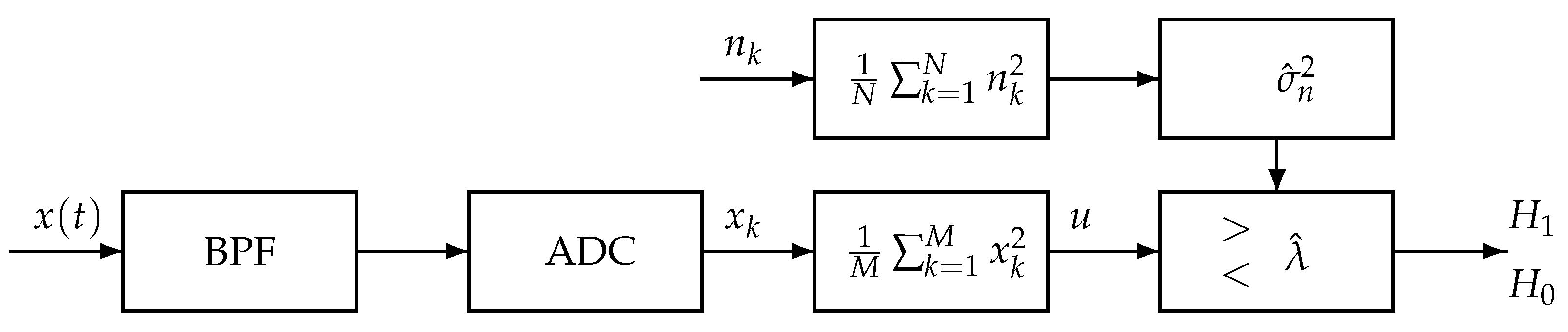
In this paper, the energy detection scheme is carried out under the framework shown in Figure 1, which is a generation of the detection scheme described in [13]. The similar part is that the input signal $x\left(t\right)$ is first passing a Band-Pass Filter (BPF) and next the signal is digitized by an analog to digital converter (ADC), then, a simple square and average device is used to estimate the received signal energy. For a real input signal, the estimated energy, $u=\frac{1}{M}{\sum }_{k=1}^M{x}_k^2$, is then compared with a threshold, $\lambda$, to decide if a signal is present ($H_1$) or not ($H_0$). The threshold for energy detection used in [13] is constructed using the information of noise variance and signal-to-noise ratio. In the proposed framework shown by Figure 1, the noise variance is estimated from another available channel, ${\widehat{\sigma }}_n^2=\frac{1}{N}{\sum }_{k=1}^N{n}_k^2$, and then the estimated noise variance is used to construct the detection threshold. This setting of detection is more applicable, since the real complicated noise is derived from various sources and thus its variance may change from time to time. Though the method using estimated noise variance to construct the threshold has been proposed in the literature, e.g., [14,15,16,17], they did not analyze the effect caused by using the estimation variance. An interesting double threshold detection method is presented in [18] using exact noise variance to separate three cases of detection: spectrum free, spectrum occupied and not certain. In this paper, we will calculate the expectation of the detection event by using the estimated variance and thus a much more accurate threshold may be derived for detection.

Figure 1. Energy detector using estimated noise variance by available similar channel. The noise variance is estimated by ${\widehat{\sigma }}_n^2=\frac{1}{N}{\sum }_{k=1}^N{n}_k^2$ from the other available similar channel. Then the empirical average energy $u=\frac{1}{M}{\sum }_{k=1}^M{x}_k^2$ is detected by principle constant false alarm rate (CFAR) or constant detection rate (CDR) with the threshold $\widehat{\lambda }$ using the estimated noise variance ${\widehat{\sigma }}_n^2$.

The threshold is determined typically based on two principles: constant false alarm rate (CFAR) and constant detection rate (CDR), which will be further explained in Section 2. In both cases, the noise variance (power) is generally supposed to be known to determine the threshold, as shown in [19,20]. However, noise variance may vary significantly in both temporal and spatial dimension due to the fact that the total noise is composed of thermal noise, receiver noise, and environmental noise. Generally, one may take the estimated noise variance, to some certain extent, as the noise variance in the calculation of the threshold in energy detection accordingly. The following two examples are given in [13] for practical performance of energy detection. One example is that a certain channel is reserved for special applications by spectrum regulators. The special channel can only be used to estimate noise variance, and can never be used by a secondary user. For instance, channel 37 (from 608 to 614 MHz) in FCC is used in very few occasions but for radioastronomy. Another example is the detection of DTV pilot signals, in which the noise variance can be estimated from some frequency bin not corresponding to the pilot frequency under the low SNR scenario. In both examples, a threshold is computed from the estimated noise variance based on CFAR or CDR principles. Then, the threshold is used in the subsequent detection to determine whether a signal is present or not by comparing with the detected energy from the channel of interest or from the known pilot frequency bin.

What are the encountered problems for detection using estimated noise variance? For CFAR principle, the resultant false alarm rate ${\widehat{P}}_{fa}$ may not be guaranteed as the preassigned level $P_{fa}$. Since the resultant rate ${\widehat{P}}_{fa}$ is actually a random variable. Indeed, the estimated noise variance ${\widehat{\sigma }}_n^2$ is a random variable. Thus the CFAR threshold, denoted by ${\widehat{\lambda }}_{fa}$, using variance ${\widehat{\sigma }}_n^2$ is also a random variable, which implies that the resulted probability of false alarm for energy detection, denoted as ${\widehat{P}}_{fa}$, is also a random variable. Obviously, it is generally impossible to expect that ${\widehat{P}}_{fa}$ equals the preassigned $P_{fa}$. Let us show a simple example here for demonstration of the theoretical results. Let $M=60$, $N=30$, if we want to set a threshold by the standard energy detection method (replacing the noise variance by its estimation) to guarantee $E{\widehat{P}}_{fa}=0.05$, the preassigned false alarm rate to set the threshold should be cautious and it is found by Theorem 1 that it should be approximately $P_{fa}^0=0.00033955$, which is much smaller than the desired rate $0.05$. However, if the sample number N increases to 100, the preassigned false alarm rate could be $P_{fa}^0=0.0129$. As the sample number N increases, the preassigned rate approaches to $0.05$ itself.

In this paper we analyze the difference between $P_{fa}$ and $E{\widehat{P}}_{fa}$. It is found in [13] that the expectation of ${\widehat{P}}_{fa}$, which is actually calculated using an approximated random variable therein, is greater than $P_{fa}$ for some predesigned $P_{fa}$, say, $0.01$, which is shown in Figure 2 therein. Hence, to make a proper choice of the threshold, it is critical to answer the following questions:

Figure 2. Plots of Examples 1 and 2. (a) Average false alarm probability ${\overline{\widehat{P}}}_{fa}>P_{fa}$ vs. P_fa = 0, 0.05, …, 1. (b) ${\overline{\widehat{P}}}_{fa}$ vs. M = N = 1, 2, …, 100

• What is the expectation of ${\widehat{P}}_{fa}$?
• What is the variance of ${\widehat{P}}_{fa}$? (equivalently, the second moment of $E{\widehat{P}}_{fa}^2$)
• What is the limitation of $E{\widehat{P}}_{fa}$ for a fixed $P_{fa}$ as N, the number of samples used to estimate the noise variance, and M, the number of samples used to perform detection, tend to infinity?

Although a part of these issues, e.g., the first and third for the case of $M=N$, have been tackled and initially studied in [13]. Yet, the study failed to find an explicit form for $E{\widehat{P}}_{fa}$, which leaves a large space for further advance. Motivated by this, we investigate the problems by explicitly describing $E{\widehat{P}}_{fa}$ and establishing an upper bound for $E{\widehat{P}}_{fa}^2$, which well answers the first issue and the second partly. Moreover, with an approximation of $E{\widehat{P}}_{fa}$ based on an estimated distribution of the resulted threshold ${\widehat{\lambda }}_{fa}$, the third question is analyzed for some special cases. Nevertheless, some new CFAR thresholds for energy detection are proposed by confirming that $E{\widehat{P}}_{fa}$ equals to the predesigned false alarm probability $P_{fa}$.

The rest of this paper is organized as follows. The model setting and hypothesis testing of energy detection by a known noise variance is introduced in Section 2, where the CFAR thresholds are derived in an exact way and an approximating way, respectively, by assuming Gaussian signals. Section 3 numerically investigates the selection of CFAR based on an estimated noise variance to set a CFAR threshold. In Section 4, we analyze some basic statistical properties of the resulted probability of false alarm ${\widehat{P}}_{fa}$ given by (21) along with ${\widehat{\tilde{P}}}_{fa}$, the estimated case given by (24). Specifically, we come up with explicit descriptions for the expectations of ${\widehat{P}}_{fa}$ and ${\widehat{\tilde{P}}}_{fa}$ by Theorems 1 and 3, respectively, and some discussions on the corresponding properties. In Section 5, upper bounds on $E{\widehat{P}}_{fa}^2$ and $E{\widehat{\tilde{P}}}_{fa}^2$ are derived by Theorems 5 and 6, respectively, due to the difficulty in finding the exact explicit forms by any known special functions. In Section 6, new CFAR thresholds are proposed, aiming to assure that $E{\widehat{P}}_{fa}$ or $E{\widehat{\tilde{P}}}_{fa}$ equals to the predetermined false alarm probability $P_{fa}$. Concluding remarks and future research are listed in Section 7. All analytical results derived in this paper are regarding CFAR thresholds. However, as a matter of fact, similar results also hold for the CDR case.

2. Model Setting and Hypothesis Testing with Known Noise Variance

Spectrum sensing is an important task for a secondary user in a cognitive radio network in order to determine whether a licensed band is currently occupied by a primary user or not. This is can be formulated into a binary hypothesis testing problem: [13,20]:

$$\begin{array}{c}\hfill x\left(k\right)=\left\{\begin{array}{cc}n\left(k\right),\hfill & H_0\left(\mathrm{vacant}\right),\hfill \\ s\left(k\right)+n\left(k\right),\hfill & H_1\left(\mathrm{occupied}\right),\hfill \end{array}\right.\end{array}$$

(1)

where $s\left(k\right)$, $n\left(k\right)$, and $x\left(k\right)$ represents the primary user’s signal, the noise, and the received signal, respectively. The noise is assumed to be Gaussian random process of zero mean and variance ${\sigma }_n^2$, whereas the signal is also assumed to be iid Gaussian random process of zero mean and variance of ${\sigma }_s^2$. The signal to noise ratio is defined as the ratio of signal variance to the noise variance

$$\begin{array}{c}\hfill \mathrm{SNR}={\sigma }_s^2/{\sigma }_n^2.\end{array}$$

(2)

The test statistics generated from the energy detector as shown in Figure 1 are

$$\begin{array}{c}\hfill u=\frac{1}{M}\sum _{k=1}^M{x}_k^2.\end{array}$$

(3)

Under the hypotheses $H_0$ and $H_1$, the test statistic u is a random variable whose probability density function (PDF) is chi-square distributed. Let us denote a chi-square distributed random variable X with M degrees of freedom as $X\sim {\chi }_M^2$, and recall its PDF as

$$\begin{array}{c}\hfill f_{\chi }(x,M)=\left\{\begin{array}{cc}\frac{1}{2^{M/2}\mathsf{\Gamma }(M/2)}{x}^{M/2-1}{e}^{-x/2},\hfill & \mathrm{for} x>0,\hfill \\ 0,\hfill & \mathrm{otherwise},\hfill \end{array}\right.\end{array}$$

(4)

where $\mathsf{\Gamma }(·)$ denotes Gamma function, given in (15).

Clearly, under hypothesis $H_0$, $Mu/{\sigma }_n^2\sim {\chi }_M^2$; and $Mu/{\sigma }_t^2\sim {\chi }_M^2$ under $H_1$ with ${\sigma }_t^2=(1+\mathrm{SNR}){\sigma }_n^2$. Thus, the PDF of test statistics u, given by test, is

$$\begin{array}{c}\hfill f_u\left(x\right)\sim \left\{\begin{array}{cc}\frac{{\sigma }_n^2}{M}{f}_{\chi }(\frac{x{\sigma }_n^2}{M},M),\hfill & \mathrm{under}{H}_0;\hfill \\ \frac{{\sigma }_t^2}{M}{f}_{\chi }(\frac{x{\sigma }_t^2}{M},M),\hfill & \mathrm{under}{H}_1.\hfill \end{array}\right.\end{array}$$

(5)

When M is sufficiently large, we can approximate the PDF of u using Gaussian distribution:

$$\begin{array}{c}\hfill {\tilde{f}}_u\left(x\right)\sim \left\{\begin{array}{cc}\mathcal{N}({\sigma }_n^2,2{\sigma }_n^4/M),\hfill & \mathrm{under}{H}_0;\hfill \\ \mathcal{N}({\sigma }_t^2,2{\sigma }_t^4/M),\hfill & \mathrm{under}{H}_1.\hfill \end{array}\right.\end{array}$$

(6)

For a given threshold $\lambda$, the probability of false alarm is given by

$$\begin{array}{c}\hfill P_{fa}=\mathrm{prob}[u>\lambda |H_0]=\mathsf{\Gamma }\left(\frac{M}{2},\frac{M\lambda }{2{\sigma }_n^2}\right),\end{array}$$

(7)

where $\mathsf{\Gamma }(a,x)$ is the upper incomplete gamma function in (16). In addition, its approximating form of $P_{fa}$ corresponding to distribution (6) for large M is

$$\begin{array}{c}\hfill {\tilde{P}}_{fa}=Q\left(\frac{\lambda -{\sigma }_n^2}{{\sigma }_n^2/\sqrt{M/2}}\right),\end{array}$$

(8)

where $Q(·)$ is defined in (14).

If the required probability of false alarm rate ($P_{fa}$) is predetermined, the threshold (${\lambda }_{fa}$) can be set accordingly by

$$\begin{array}{c}\hfill {\lambda }_{fa}=\frac{2{\sigma }_n^2}{M}{\mathsf{\Gamma }}^{-1}\left(M/2,P_{fa}\right),\end{array}$$

(9)

where ${\mathsf{\Gamma }}^{-1}(a,x)$ is the inverse function of $\mathsf{\Gamma }(a,x)$. Furthermore, for the approximation case:

$$\begin{array}{c}\hfill {\tilde{\lambda }}_{fa}={\sigma }_n^2\left(1+\frac{Q^{-1}\left(P_{fa}\right)}{\sqrt{M/2}}\right),\end{array}$$

(10)

where $Q^{-1}\left(x\right)$ is the inverse function of $Q\left(x\right)$.

Similarly, under hypothesis $H_1$, for a given threshold $\lambda$, the probability of detection is given by

$$\begin{array}{c}\hfill P_d=\mathrm{prob}[u>\lambda |H_1]=\mathsf{\Gamma }\left(\frac{M}{2},\frac{M\lambda }{2{\sigma }_t^2}\right),\end{array}$$

(11)

where $\mathsf{\Gamma }(a,x)$ is the upper incomplete gamma function. So, we derive the threshold to achieve a target probability of detection at the required signal level or SNR:

$$\begin{array}{c}\hfill {\lambda }_d=\frac{2{\sigma }_n^2(1+\mathrm{SNR})}{M}{\mathsf{\Gamma }}^{-1}\left(M/2,P_d\right).\end{array}$$

(12)

Furthermore, the corresponding approximating case is

$$\begin{array}{c}\hfill {\tilde{\lambda }}_d={\sigma }_n^2(1+\mathrm{SNR})\left(1+\frac{Q^{-1}\left(P_d\right)}{\sqrt{M/2}}\right).\end{array}$$

(13)

The probability of false alarm is fixed to a small value (e.g., 5%) if it is required to guarantee a reuse probability of the unused spectrum, and meanwhile the detection probability should be maximized as much as possible. This is referred to as constant false alarm rate (CFAR) principle [13,19]. On the other hand, if it is required to guarantee a non-interference probability to the primary users, the probability of detection should be set to a high level (e.g., 95%) and the probability of false alarm should be minimized as much as possible. This is called the constant detection rate (CDR) principle [13,19]. By the similarity of (9) and (12), it is clear that the derivation of the threshold values for CFAR and CDR are similar, so the analytic results derived by assuming CFAR based detection can be applied to CDR based detection with minor modifications and vice versa. From now on, we will mainly focus on the discussion of CFAR threshold, since similar conclusions follow directly by minor changes.

Let us introduce some special functions and related notations for ease of reading. The complement of the standard normal distribution function is often denoted as $Q\left(x\right)$, i.e.,

$$\begin{array}{c}\hfill Q\left(x\right)={\int }_x^{\infty }\frac{1}{\sqrt{2\pi }}{e}^{-\frac{t^2}{2}}dt,\end{array}$$

(14)

and is simply referred to as Q-function, in the context of engineering. This represents the tail probability of the standard Gaussian distribution. The Gamma function and regularized upper incomplete Gamma function are defined as

$$\begin{array}{c}\mathsf{\Gamma }\left(k\right)={\int }_0^{\infty }{t}^{k-1}{e}^{-t}dt,\hfill \end{array}$$

(15)

$$\begin{array}{c}\mathsf{\Gamma }(k,x)=\frac{1}{\mathsf{\Gamma }\left(k\right)}{\int }_x^{\infty }{t}^{k-1}{e}^{-t}dt\hfill \end{array}$$

(16)

for $k>0$, respectively. The more complicated Beta function and Beta distribution function are respectively listed below

$$\begin{array}{c}B(a,b)={\int }_0^1{t}^{a-1}{(1-t)}^{b-1}dt,\hfill \end{array}$$

(17)

$$\begin{array}{c}B(x,a,b)=\frac{1}{B(a,b)}{\int }_0^x{t}^{a-1}{(1-t)}^{b-1}dt.\hfill \end{array}$$

(18)

for $a>0$, $b>0$ and $x\in [0,1]$. A well-known relation between Beta and Gamma function is

$$\begin{array}{c}\hfill B(a,b)=\frac{\mathsf{\Gamma }\left(a\right)\mathsf{\Gamma }\left(b\right)}{\mathsf{\Gamma }(a+b)}.\end{array}$$

We simply use $Q^{-1}\left(x\right)$, ${\mathsf{\Gamma }}^{-1}(k,x)$ and $B^{-1}(x,a,b)$ to present the inverse functions of $Q\left(x\right)$, $\mathsf{\Gamma }(k,x)$ and $B(x,a,b)$ respectively.

3. Energy Detection Performance Using Estimated Noise Variance

As already mentioned in the introduction, the exact noise variance is generally unavailable; even historic records are sometimes out of use, due to timely changes of thermal conditions and environmental conditions, and so on. So, practically the threshold values in (9) and (12), or the approximating cases (10) and (13), are usually calculated from an estimated noise variance ${\widehat{\sigma }}_n^2$ to a certain extent. In this section, we numerically study the performance of energy detection by replacing the noise variance in these formulas by an estimated noise variance ${\widehat{\sigma }}_n^2$. Specifically, we investigate the difference $E{\widehat{P}}_{fa}-P_{fa}$ by numerical experiments.

We want to find out the performance of energy detection by simply replacing the exact noise variance ${\sigma }_n^2$ in (9) and (12) with the estimated noise variance ${\widehat{\sigma }}_n^2$, i.e., calculate the thresholds as

$$\begin{array}{c}{\widehat{\lambda }}_{fa}=\frac{2{\widehat{\sigma }}_n^2}{M}{\mathsf{\Gamma }}^{-1}\left(M/2,P_{fa}\right),\hfill \end{array}$$

(19)

$$\begin{array}{c}{\widehat{\lambda }}_d=\frac{2{\widehat{\sigma }}_n^2(1+\mathrm{SNR})}{M}{\mathsf{\Gamma }}^{-1}\left(M/2,P_d\right),\hfill \end{array}$$

(20)

and then by (7) and (11) respectively the resulted performance probabilities are

$$\begin{array}{c}{\widehat{P}}_{fa}=\mathrm{prob}[u>{\widehat{\lambda }}_{fa}|H_0]=\mathsf{\Gamma }\left(\frac{M}{2},\frac{M{\widehat{\lambda }}_{fa}}{2{\sigma }_n^2}\right),\hfill \end{array}$$

(21)

$$\begin{array}{c}{\widehat{P}}_d=\mathrm{prob}[u>{\widehat{\lambda }}_d|H_1]=\mathsf{\Gamma }\left(\frac{M}{2},\frac{M{\widehat{\lambda }}_d}{2{\sigma }_t^2}\right).\hfill \end{array}$$

(22)

Similarly, in the approximating case, the CFAR threshold ${\tilde{\lambda }}_{fa}$ by replacing with the estimated noise variance ${\widehat{\sigma }}_n^2$ is

$$\begin{array}{c}\hfill {\widehat{\tilde{\lambda }}}_{fa}={\widehat{\sigma }}_n^2\left(1+\frac{Q^{-1}\left(P_{fa}\right)}{\sqrt{M/2}}\right),\end{array}$$

(23)

which is corresponding to (10). Thus the resulted performance probability is

$$\begin{array}{c}\hfill {\widehat{\tilde{P}}}_{fa}=\mathrm{prob}[u>{\widehat{\tilde{\lambda }}}_{fa}]=Q\left(\frac{{\widehat{\tilde{\lambda }}}_{fa}-{\sigma }_n^2}{{\sigma }_n^2/\sqrt{M/2}}\right).\end{array}$$

(24)

Due to the CFAR and CDR principles having an essentially similar structure, we actually investigate the CFAR case only, i.e., by formulas (19) and (21) to check the evolvement of $E{\widehat{P}}_{fa}$ as the predetermined $P_{fa}$ varying from 0 to 1, or for a fixed $P_{fa}$ as the number of samples tends to infinity. A technical treatment of estimating $E{\widehat{P}}_{fa}$ in the following experiments is replacing it by the corresponding empirical average ${\overline{\widehat{P}}}_{fa}$ over a class of sample paths.

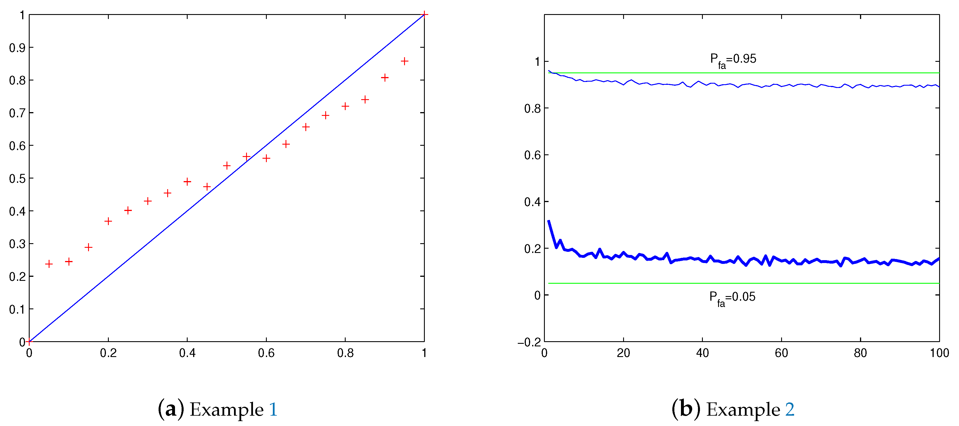
Example 1.

We first investigate the difference between $E{\widehat{P}}_{fa}$ and the predesigned $P_{fa}$ as $P_{fa}$ changes along the interval $[0,1]$ with M and N fixed. In model (1), let ${\sigma }_n^2=1$ and $M=60$. Consider a given false alarm rate $P_{fa}$, we use $N=30$ iid Gaussian noises to estimate the variance ${\widehat{\sigma }}_n^2$, and then substitute ${\widehat{\sigma }}_n^2$ in (19) to derive the threshold ${\widehat{\lambda }}_{fa}$. The energy detection performance by the obtained threshold ${\widehat{\lambda }}_{fa}$ is evaluated by the corresponding false alarm probability ${\widehat{P}}_{fa}$ by (21). As aforementioned, it is important to check whether $E{\widehat{P}}_{fa}=P_{fa}$. In order to estimate $E{\widehat{P}}_{fa}$, repeat independently the aforementioned procedure and calculation for 600 times to calculate the average false alarm probability

$${\overline{\widehat{P}}}_{fa}=\frac{1}{600}\sum _{i=1}^{600}{\widehat{P}}_{fa}\left({\omega }_i\right)$$

to serve as an empirical approximation of $E{\widehat{P}}_{fa}$, where ${\widehat{P}}_{fa}\left({\omega }_i\right)$ denotes the calculated probability along the i-th sample path $\omega \left(i\right)$. We let $P_{fa}=0,0.05,\dots ,1$, totally 21 points, to do an experiment. The result is shown in Figure 2a, where ${\overline{\widehat{P}}}_{fa}$ is plotted by ’+’. We see that ${\overline{\widehat{P}}}_{fa}>P_{fa}$ when $P_{fa}$ is close to 0, while ${\overline{\widehat{P}}}_{fa}<P_{fa}$ when $P_{fa}$ is near 1.

Example 2.

This time we investigate the difference between $E{\widehat{P}}_{fa}$ and the predesigned $P_{fa}$ with a fixed $P_{fa}$ as $M=N$ tends to infinity. Still let ${\sigma }_n^2=1$ in model (1). With the same procedure of Example 1 to calculate ${\overline{\widehat{P}}}_{fa}$ by 600 independent sample paths. We let $P_{fa}=0.05$ and $0.95$ respectively, and $M=N=1,2,\dots ,100$ to do an experiment. The result is shown in Figure 2b, where ${\overline{\widehat{P}}}_{fa}$ for $P_{fa}=0.05$ is plotted by thick line, and $P_{fa}=0.95$ by ordinary line. We see that ${\overline{\widehat{P}}}_{fa}>P_{fa}$ when $P_{fa}=0.05$, and ${\overline{\widehat{P}}}_{fa}<P_{fa}$ when $P_{fa}=0.95$. Furthermore, it seems that ${\overline{\widehat{P}}}_{fa}$, and thus $E{\widehat{P}}_{fa}$, for a fixed $P_{fa}$ has a limitation as $M=N$ tends to infinity.

The phenomena discovered by these numerical experiments will be explained in the next two sections by developing an exact formula for $E{\widehat{P}}_{fa}$ and an upper bound for its variance. Nevertheless, the case for approximating CFAR threshold has also been analyzed meanwhile.

4. Calculations of $E{\widehat{P}}_{fa}$ and $E{\widehat{\tilde{P}}}_{fa}$

In this section, we will derive explicit formulas for the expectation of ${\widehat{P}}_{fa}$ given by (19) and (21) with respect to predesigned false alarm probability $P_{fa}$, and the expectation of ${\widehat{\tilde{P}}}_{fa}$ given by (23) and (24). Moreover, some basic properties are deduced analytically and numerically, which further explains some discoveries in the former section.

Denote $Y=\frac{1}{N}{\sum }_{k=1}^N{Y}_k^2$ as the estimated noise variance from the reference channel (Ch${}_0$) known to be vacant, where N is the number of samples used to estimate noise variance. Denote u by (3) as the energy detection test statistics from the channel of interest (Ch${}_1$). Here we assume the number of samples, as aforementioned, used to perform spectrum sensing is M.

Notice that the estimated noise variance, $Y=\frac{1}{N}{\sum }_{k=1}^N{Y}_k^2$, is a random variable itself, the probability of false alarm or detection is conditioned on one observation of the random variable, e.g., y. Let us consider the case of CFAR. By (7) and (19), the probability of false alarm can be written as

$$\begin{array}{c}\hfill {\widehat{P}}_{fa}=\mathrm{prob}[u>{\widehat{\lambda }}_{fa}]=\mathsf{\Gamma }\left(\frac{M}{2},\frac{y}{{\sigma }_n^2}{\mathsf{\Gamma }}^{-1}\left(M/2,P_{fa}\right)\right),\end{array}$$

(25)

where ${\widehat{\lambda }}_{fa}$ is the threshold value calculated from (19) by given false alarm probability $P_{fa}$, and y is a realization of random variable Y.

Since ${\widehat{P}}_{fa}$ given by (25) is a random variable depending on y, it is natural to consider its expectation with respect to y. Let us summarize a theoretical result regarding $E{\widehat{P}}_{fa}$ as a theorem below.

Theorem 1.

When using estimated threshold ${\widehat{\lambda }}_{fa}$ of CFAR given by (19) for model (1), we have

$$\begin{array}{c}\hfill E{\widehat{P}}_{fa}=B\left(\frac{N}{N+2x},\frac{N}{2},\frac{M}{2}\right),\end{array}$$

(26)

where $x={\mathsf{\Gamma }}^{-1}\left(M/2,P_{fa}\right)$ and Beta distribution $B(x,a,b)$ is defined by (18).

Proof of Theorem 1.

By integrating (25) over the PDF of Y, the expected probability of false alarm can be derived as

$$\begin{array}{ll}E{\widehat{P}}_{fa}& =E\mathsf{\Gamma }\left(\frac{M}{2},\frac{y}{{\sigma }_n^2}{\mathsf{\Gamma }}^{-1}\left(M/2,P_{fa}\right)\right)\\ & ={\int }_0^{\infty }\mathsf{\Gamma }\left(\frac{M}{2},\frac{t}{N}{\mathsf{\Gamma }}^{-1}\left(M/2,P_{fa}\right)\right)f_{\chi }\left(t,N\right)dt,\end{array}$$

(27)

where we use the fact $t=Ny/{\sigma }_n^2\sim {\chi }_N^2$ in the second step. Letting $x={\mathsf{\Gamma }}^{-1}\left(M/2,P_{fa}\right)$, we derive

$$\begin{array}{ll}E{\widehat{P}}_{fa}& ={\int }_0^{\infty }\mathsf{\Gamma }\left(M/2,tx/N\right)f_{\chi }\left(t,N\right)dt\\ & ={\int }_0^{\infty }\frac{1}{\mathsf{\Gamma }(M/2)}{\int }_{tx/N}^{\infty }{s}^{M/2-1}{e}^{-s}ds\frac{1}{2^{N/2}\mathsf{\Gamma }(N/2)}{t}^{N/2-1}{e}^{-t/2}dt.\end{array}$$

(28)

Differentiating by x, we have

$$\begin{array}{ll}\frac{d\left(E{\widehat{P}}_{fa}\right)}{dx}& =\frac{-1}{\mathsf{\Gamma }\left(\frac{M}{2}\right)\mathsf{\Gamma }\left(\frac{N}{2}\right)2^{N/2}}{\int }_0^{\infty }{\left(\frac{tx}{N}\right)}^{M/2-1}{e}^{-\frac{tx}{N}}\frac{t}{N}{t}^{N/2-1}{e}^{-t/2}dt\\ & =\frac{-x^{M/2-1}{(1/N)}^{M/2}}{\mathsf{\Gamma }\left(\frac{M}{2}\right)\mathsf{\Gamma }\left(\frac{N}{2}\right)2^{N/2}}{\int }_0^{\infty }{t}^{\frac{M+N}{2}-1}{e}^{-\left(\frac{x}{N}+\frac{1}{2}\right)t}dt.\end{array}$$

(29)

Introduce transformation $u=\left(\frac{x}{N}+\frac{1}{2}\right)t$. By the fact that $x>0$, we proceed as

$$\begin{array}{ll}\frac{d\left(E{\widehat{P}}_{fa}\right)}{dx}& =\frac{-x^{M/2-1}{(1/N)}^{M/2}}{\mathsf{\Gamma }\left(\frac{M}{2}\right)\mathsf{\Gamma }\left(\frac{N}{2}\right)2^{N/2}}·\frac{1}{{\left(\frac{x}{N}+\frac{1}{2}\right)}^{\frac{M+N}{2}}}{\int }_0^{\infty }{u}^{\frac{M+N}{2}-1}{e}^{-u}du\\ & =\frac{-x^{M/2-1}{(1/N)}^{M/2}}{2^{N/2}{\left(\frac{x}{N}+\frac{1}{2}\right)}^{\frac{M+N}{2}}}·\frac{\mathsf{\Gamma }\left(\frac{M+N}{2}\right)}{\mathsf{\Gamma }\left(\frac{M}{2}\right)\mathsf{\Gamma }\left(\frac{N}{2}\right)}\\ & =\frac{-x^{M/2-1}{(1/N)}^{M/2}{(1/2)}^{N/2}}{B(\frac{M}{2},\frac{N}{2}){\left(\frac{x}{N}+\frac{1}{2}\right)}^{\frac{M+N}{2}}},\end{array}$$

(30)

where $B(\frac{M}{2},\frac{N}{2})$ is Beta function in (17). Integrating (30) over $(x,\infty )$, by noticing $E{\widehat{P}}_{fa}=0$ for $x=\infty$ in (27), we derive

$$\begin{array}{cc}\hfill E{\widehat{P}}_{fa}& ={\int }_x^{\infty }\frac{u^{M/2-1}{(1/N)}^{M/2}{(1/2)}^{N/2}}{B(\frac{M}{2},\frac{N}{2}){\left(\frac{u}{N}+\frac{1}{2}\right)}^{\frac{M+N}{2}}}du.\hfill \end{array}$$

(31)

Let $w=\frac{2u}{N}$. The integral turns to be

$$\begin{array}{ll}E{\widehat{P}}_{fa}& =\frac{1}{B(\frac{M}{2},\frac{N}{2})}{\int }_{\frac{2x}{N}}^{\infty }\frac{w^{\frac{M}{2}-1}}{{(w+1)}^{\frac{M+N}{2}}}dw\\ & =\frac{1}{B(\frac{M}{2},\frac{N}{2})}{\int }_0^{\frac{N}{N+2x}}{s}^{\frac{N}{2}-1}{(1-s)}^{\frac{M}{2}-1}ds\\ & =B\left(\frac{N}{N+2x},\frac{N}{2},\frac{M}{2}\right),\end{array}$$

(32)

where $B(x,a,b)$ is the Beta distribution function in (18). In the second step, we use the transformation $w=\frac{1}{s}-1$.  □

Based on Theorem 1, we conclude a further theoretical discovery as the following theorem, which is actually being pointed out in the numerical experiments of the former section.

Theorem 2.

There exists a $p_0\in \left(0,1\right)$ such that

$$\begin{array}{c}\hfill E{\widehat{P}}_{fa}>P_{fa}for P_{fa}\in (0,p_0),E{\widehat{P}}_{fa}<P_{fa}for P_{fa}\in (p_0,1),\end{array}$$

(33)

where $E{\widehat{P}}_{fa}$ is defined by (27), and can be calculated by (26).

Proof. 

Let $P_{fa}=p$ to be brief. Introduce a function $\psi \left(p\right)=E{\widehat{P}}_{fa}-p$. By (26), we have

$$\begin{array}{ll}{\psi }^{\prime }\left(p\right)& =\frac{d\left(B\left(\frac{N}{N+2x},\frac{N}{2},\frac{M}{2}\right)\right)}{dx}·\frac{dx}{dp}-1\\ & =\frac{1}{B(\frac{N}{2},\frac{M}{2})}{\left(\frac{N}{N+2x}\right)}^{\frac{N}{2}-1}{\left(\frac{2x}{N+2x}\right)}^{\frac{M}{2}-1}·\frac{2N\mathsf{\Gamma }(M/2)x^{1-\frac{M}{2}}{e}^x}{{(N+2x)}^2}-1\\ & =\frac{C(M,N)e^x}{{(N+2x)}^{\frac{M+N}{2}}}-1,\end{array}$$

(34)

where $C(M,N)=\frac{\mathsf{\Gamma }\left(\frac{M+N}{2}\right)}{\mathsf{\Gamma }\left(\frac{N}{2}\right)}{N}^{\frac{N}{2}}{2}^{\frac{M}{2}}$. By the fact $x={\mathsf{\Gamma }}^{-1}\left(M/2,p\right)$, i.e., $p=\mathsf{\Gamma }(M/2,x)$, we have used the following calculation

$$\begin{array}{c}\hfill \frac{dx}{dp}=\frac{1}{\frac{dp}{dx}}=\frac{-\mathsf{\Gamma }(M/2)}{x^{\frac{M}{2}-1}{e}^{-x}}\end{array}$$

in the above second step. Note $x=\infty$ when $p=0$, so ${\psi }^{\prime }\left(0\right)>0$ by (34). Note further $x=0$ if $p=1$, by (34) we have ${\psi }^{\prime }\left(1\right)>0$. Together with the fact that $\psi \left(0\right)=\psi \left(1\right)=0$, we know that ${\psi }^{\prime }$ is negative somewhere.

To find more information about the sign of ${\psi }^{\prime }\left(x\right)$, we recall the famous Stirling’s approximation formula for Gamma function (see page 400 of [21]):

$$\begin{array}{c}\hfill \mathsf{\Gamma }(n+1)=\sqrt{2\pi n}{\left(\frac{n}{e}\right)}^n{e}^{{\lambda }_n}\end{array}$$

(35)

where $\frac{1}{12n+1}<{\lambda }_n<\frac{1}{12n}$, and an inequality (see page 88 of [21]):

$$\begin{array}{c}\hfill {\left(1+\frac{1}{n}\right)}^{n+\alpha }\le e\le {\left(1+\frac{1}{n}\right)}^{n+\beta },\end{array}$$

(36)

where $\alpha \le \frac{1}{ln2}-1=0.4427\cdots$ and $\beta \ge \frac{1}{2}$.

By (35), we get

$$\begin{array}{c}\hfill C(M,N)=e^{\theta }\sqrt{\frac{M+N-2}{N-2}}\frac{{(M+N-2)}^{\frac{M+N}{2}-1}{N}^{\frac{N}{2}}}{{(N-2)}^{\frac{N}{2}-1}{e}^{\frac{M}{2}}}\end{array}$$

with $\theta \in \left(\frac{-6M-1}{\left(6\right(M+N)-11)(6N-12)},\frac{-6M+1}{\left(6\right(M+N)-12)(6N-11)}\right)$. Thus,

$$\begin{array}{c}\hfill {\psi }^{\prime }\left(p\right)=e^{\theta }\sqrt{\frac{M+N-2}{N-2}}\frac{{(M+N-2)}^{\frac{M+N}{2}-1}{N}^{\frac{N}{2}}}{{(N+2x)}^{\frac{M+N}{2}}{(N-2)}^{\frac{N}{2}-1}}{e}^{x-\frac{M}{2}}-1.\end{array}$$

By (36),

$$\begin{array}{c}\hfill {\left(\frac{N}{N-2}\right)}^{\frac{N}{2}-1}={\left(1+\frac{2}{N-2}\right)}^{\frac{N-2}{2}}<e.\end{array}$$

Together with the facts that $e^{\theta }<1$ and

$$\begin{array}{c}\hfill \frac{N}{\sqrt{(N-2)(M+N-2)}}<1\end{array}$$

for $M\ge 6$, we declare that the derivative of $\psi \left(p\right)$ at p, corresponding $x=\frac{M}{2}-1$, i.e., ${\psi }^{\prime }\left({\mathsf{\Gamma }}^{-1}(\frac{M}{2},\frac{M}{2}-1)\right)<0$.

On the other hand, by noticing the increase rates of function $e^x$ and ${(N+2x)}^{\frac{M+N}{2}}$ in (34), we know that ${\psi }^{\prime }\left(p\right)$ at most has two zeros in $(0,1)$. Hence, we conclude that ${\psi }^{\prime }\left(p\right)$ starts as a positive value ${\psi }^{\prime }\left(0\right)>0$, then decreases to a negative minimum, and finally increases to a positive value ${\psi }^{\prime }\left(1\right)>0$. This means that $\psi \left(p\right)$ starts as 0 increases to a positive maximum, and then decreases to negative minimum, finally increases to 0, which is just the assertion desired.  □

Now let us consider the counterparts for the approximating threshold of CFAR criterion, i.e., the expectation of ${\widehat{\tilde{P}}}_{fa}$ given by (23) and (24).

Theorem 3.

When using estimated threshold ${\widehat{\tilde{\lambda }}}_{fa}$ of CFAR given by (23) for model (1), we have

$$\begin{array}{c}\hfill E{\widehat{\tilde{P}}}_{fa}=Q\left(\frac{x\sqrt{N/2}}{\sqrt{A\left(x\right)}}\right)-Q\left(\sqrt{\frac{N}{2}}\right),\end{array}$$

(37)

where $A\left(x\right)=x^2+x\sqrt{2M}+\frac{M+N}{2}$ and $x=Q^{-1}\left(P_{fa}\right)$.

Remark 1.

Based on Theorem 3, we now consider the limitation of $E{\widehat{\tilde{P}}}_{fa}$ as M and N tend to infinity for fixed $P_{fa}$. By (37), for a fixed $x=Q^{-1}\left(P_{fa}\right)$, we have

$$\begin{array}{c}\hfill \underset{M,N\to \infty }{lim}E{\widehat{\tilde{P}}}_{fa}=Q\left(\frac{x}{\sqrt{1+\mu }}\right).\end{array}$$

(38)

if $M=\mu N$. Thus, if $M=N$ tends to infinity, we derive the discovery in [13]:

$$\begin{array}{c}\hfill \underset{M=N\to \infty }{lim}E{\widehat{\tilde{P}}}_{fa}=Q\left(\frac{x}{\sqrt{2}}\right).\end{array}$$

(39)

These properties also hold for $E{\widehat{P}}_{fa}$ since the distribution of ${\widehat{P}}_{fa}$ tends to be the distribution of ${\widehat{\tilde{P}}}_{fa}$.

Proof of Theorem 3.

Integrating (24) with respect to y, and noticing that $y\sim \mathcal{N}({\sigma }_n^2,2{\sigma }_n^4/N)$, we have

$$\begin{array}{c}\hfill E{\widehat{\tilde{P}}}_{fa}={\int }_{R}Q\left(\frac{y(1+Q^{-1}\left(P_{fa}\right)/\sqrt{M/2})-{\sigma }_n^2}{{\sigma }_n^2/\sqrt{M/2}}\right)\frac{1}{\sqrt{2\pi }{\sigma }_n^2/\sqrt{N/2}}{e}^{-\frac{{(y-{\sigma }_n^2)}^2}{4{\sigma }_n^4/N}}dy.\end{array}$$

(40)

Letting $x=Q^{-1}\left(P_{fa}\right)$ and $t=(y-{\sigma }_n^2)/{\sigma }_n^2$. we derive

$$\begin{array}{c}\hfill E{\widehat{\tilde{P}}}_{fa}={\int }_{R}Q(t\sqrt{M/2}+(t+1)x)\frac{\sqrt{N/2}}{\sqrt{2\pi }}{e}^{-\frac{N{t}^2}{4}}dt.\end{array}$$

(41)

For simplicity, introduce $\alpha =\sqrt{M/2}$ and $\beta =\sqrt{N/2}$. Differentiating ${\overline{\tilde{P}}}_{fa}$ over x, we get

$$\begin{array}{ll}\frac{d\left(E{\widehat{\tilde{P}}}_{fa}\right)}{dx}& ={\int }_R\frac{\partial Q(\alpha t+tx+x)}{\partial x}\frac{\beta }{\sqrt{2\pi }}{e}^{-\frac{{\left(\beta t\right)}^2}{2}}dt\\ & =-{\int }_R\frac{t+1}{\sqrt{2\pi }}{e}^{-\frac{{(\alpha t+tx+x)}^2}{2}}\frac{\beta }{\sqrt{2\pi }}{e}^{-\frac{{\left(\beta t\right)}^2}{2}}dt\\ & =-\frac{\beta }{2\pi }{\int }_R(1+t)exp\left\{-\frac{1}{2}[x^2+2xt(x+\alpha )+A{t}^2]\right\}dt,\end{array}$$

(42)

where $A\left(x\right)={(x+\alpha )}^2+{\beta }^2$ and hereafter denote A sometimes for brief. It follows

$$\begin{array}{ll}\frac{d\left(E{\widehat{\tilde{P}}}_{fa}\right)}{dx}& =-\frac{\beta }{2\pi }{\int }_R(1+t)exp\left\{-\frac{1}{2}\left[A{\left(t+\frac{x(x+\alpha )}{A}\right)}^2+\frac{{\left(\beta x\right)}^2}{A}\right]\right\}dt\\ & =-\frac{\beta }{2\pi }{e}^{-\frac{{\left(\beta x\right)}^2}{2A}}{\int }_R\left(1+u-\frac{x(x+\alpha )}{A}\right)e^{-\frac{A}{2}{u}^2}du\\ & =-\frac{\beta }{2\pi }{e}^{-\frac{{\left(\beta x\right)}^2}{2A}}\left(1-\frac{x(x+\alpha )}{A}\right){\int }_R{e}^{-\frac{A}{2}{u}^2}du\\ & =-\frac{\beta }{2\pi }{e}^{-\frac{{\left(\beta x\right)}^2}{2A}}\left(1-\frac{x(x+\alpha )}{A}\right)·\sqrt{\frac{2\pi }{A}}\\ & =-\frac{\beta }{\sqrt{2\pi }}{e}^{-\frac{{\left(\beta x\right)}^2}{2A}}\frac{\alpha x+{\alpha }^2+{\beta }^2}{A\sqrt{A}}\\ & =-\frac{1}{\sqrt{2\pi }}{e}^{-\frac{{\left(\beta x\right)}^2}{2A}}·{\left(\frac{\beta x}{\sqrt{A}}\right)}^{\prime }.\end{array}$$

(43)

In the second step we use the transformation $u=t+\frac{x(x+\alpha )}{A}$ to simplify the expression.

Now integrating (43) over $(x,\infty )$, and by the fact that $E{\widehat{\tilde{P}}}_{fa}=0$ for $x=\infty$ in (40), we find

$$\begin{array}{ll}E{\widehat{\tilde{P}}}_{fa}& ={\int }_x^{\infty }\frac{1}{\sqrt{2\pi }}{e}^{-\frac{{\left(\beta v\right)}^2}{2A\left(v\right)}}·{\left(\frac{\beta v}{\sqrt{A\left(v\right)}}\right)}^{\prime }dv\\ & ={\int }_x^{\infty }\frac{1}{\sqrt{2\pi }}{e}^{-\frac{{\left(\beta v\right)}^2}{2A\left(v\right)}}d\left(\frac{\beta v}{\sqrt{A\left(v\right)}}\right).\end{array}$$

(44)

Let us study the function $\varphi \left(x\right)=\frac{\beta x}{\sqrt{A\left(x\right)}}$ before introducing a transformation. Clearly,

$$\begin{array}{c}\hfill \underset{x\to -\infty }{lim}\varphi \left(x\right)=-\beta ,\underset{x\to \infty }{lim}\varphi \left(x\right)=\beta ,{\varphi }^{\prime }\left(x\right)=\frac{1}{A\sqrt{A}}(\alpha x+{\alpha }^2+{\beta }^2).\end{array}$$

Note $A>0$ and denote $x_0=-\frac{{\alpha }^2+{\beta }^2}{\alpha }$, we derive ${\varphi }^{\prime }\left(x\right)<0$ for $x<x_0$, and ${\varphi }^{\prime }\left(x\right)>0$ for $x>x_0$. Thus, $\varphi \left(x\right)$ has one unique minimum at $x_0$. Hence, $\varphi \left(x\right)$ increases from the minimum to $-\beta$ as $x\to -\infty$, and increases from the minimum to $\beta$ as $x\to \infty$.

Now introduce a transformation for (44) as $w=\varphi \left(v\right)$. Based on the above analysis for function $\varphi (·)$, if the integration region $[x,\infty )\subseteq [x_0,\infty )$, then the region for w turns to be $\left[\varphi \right(x),\beta )$; otherwise, the region for v can be divided into two monotonic parts as $[x,x_0]$ and $[x_0,\infty )$, and thus, the regions for w are $[\varphi \left(x\right),\varphi \left(x_0\right)]$ and $[\varphi \left(x_0\right),\beta )$. Then, for the case $x\ge x_0$, by the fact that ${\overline{\tilde{P}}}_{fa}=0$ for $x=\infty$ in (41), we proceed (44) as

$$\begin{array}{cc}\hfill E{\widehat{\tilde{P}}}_{fa}& ={\int }_{\varphi \left(x\right)}^{\beta }\frac{1}{\sqrt{2\pi }}{e}^{-\frac{w^2}{2}}dw=Q\left(\varphi \left(x\right)\right)-Q\left(\beta \right).\hfill \end{array}$$

(45)

For the case $x<x_0$, similarly,

$$\begin{array}{ll}E{\widehat{\tilde{P}}}_{fa}& =\left({\int }_{\varphi \left(x\right)}^{\varphi \left(x_0\right)}+{\int }_{\varphi \left(x_0\right)}^{\beta }\right)\frac{1}{\sqrt{2\pi }}{e}^{-\frac{w^2}{2}}dw\\ & =Q\left(\varphi \right(x\left)\right)-Q\left(\beta \right).\end{array}$$

These finish the proof.  □

Corresponding to Theorem 2, we also have:

Theorem 4.

There exists a ${\tilde{p}}_0\in \left(0,\frac{1}{2}\right)$ such that

$$\begin{array}{c}\hfill E{\widehat{\tilde{P}}}_{fa}>P_{fa}for P_{fa}\in (0,{\tilde{p}}_0),E{\widehat{\tilde{P}}}_{fa}<P_{fa}for P_{fa}\in ({\tilde{p}}_0,1),\end{array}$$

(46)

where $E{\widehat{\tilde{P}}}_{fa}$ can be calculated by (37). Furthermore, the critical point ${\tilde{p}}_0$ is close to $\frac{1}{2}$ for large $M,N$.

Remark 2.

By Theorem 4, we know that $E{\widehat{\tilde{P}}}_{fa}=P_{fa}$ at a point close to $p=\frac{1}{2}$. This property holds for $E{\widehat{P}}_{fa}$ since the distribution of ${\widehat{P}}_{fa}$ tends to that of ${\widehat{\tilde{P}}}_{fa}$.

Proof. 

Let $P_{fa}=p$ to be brief. Introduce a function

$$\phi \left(p\right)=E{\widehat{\tilde{P}}}_{fa}-p=Q\left(\frac{x\sqrt{N/2}}{\sqrt{A\left(x\right)}}\right)-Q\left(\sqrt{\frac{N}{2}}\right)-Q\left(x\right),$$

where $x=Q^{-1}\left(p\right)$. So, we have

$$\begin{array}{ll}\frac{d\phi }{dp}& =-\frac{1}{\sqrt{2\pi }}{e}^{-\frac{{\left(\beta x\right)}^2}{2A}}·{\left(\frac{\beta x}{\sqrt{A}}\right)}^{\prime }·\frac{dx}{dp}-1\\ & =\frac{\alpha x+{\alpha }^2+{\beta }^2}{A\sqrt{A}}\beta e^{\frac{x^2{(x+\alpha )}^2}{2A}}-1,\end{array}$$

where $x=Q^{-1}\left(p\right)$, $A={(x+\alpha )}^2+{\beta }^2$, $\alpha =\sqrt{M/2}$, and $\beta =\sqrt{N/2}$. Clearly, $x=\infty$ is corresponding to $p=0$, thus, ${\phi }^{\prime }\left(0\right)>0$. Together with the facts that $\phi \left(0\right)=0$ and $\phi \left(\frac{1}{2}\right)=-Q\left(\beta \right)<0$, we know that there exists a ${\tilde{p}}_0\in (0,\frac{1}{2})$ such that $\phi \left({\tilde{p}}_0\right)=0$. When $x<0$, corresponding to $p>\frac{1}{2}$, clearly,

$$\frac{\beta }{\sqrt{A}}<1$$

for $x<0$, we have $Q\left(x\beta /\sqrt{A}\right)-Q\left(\beta \right)<0$, and thus $\phi \left(p\right)<0$ for $p>\frac{1}{2}$, which finishes the proof of the first assertion.

By (38), i.e.,

$$\begin{array}{c}\hfill \underset{M=\mu N\to \infty }{lim}E{\widehat{\tilde{P}}}_{fa}=Q\left(\frac{x}{\sqrt{1+\mu }}\right),\end{array}$$

we have

$$\begin{array}{c}\hfill \underset{M=\mu N\to \infty }{lim}\phi \left(p\right)=Q\left(\frac{x}{\sqrt{1+\mu }}\right)-Q\left(x\right).\end{array}$$

Thus, for large M and N, we know that the zero of $\phi \left(p\right)$, i.e., ${\tilde{p}}_0$, is close to $p=\frac{1}{2}$, which is corresponding to $x=0$. This finishes the second assertion.  □

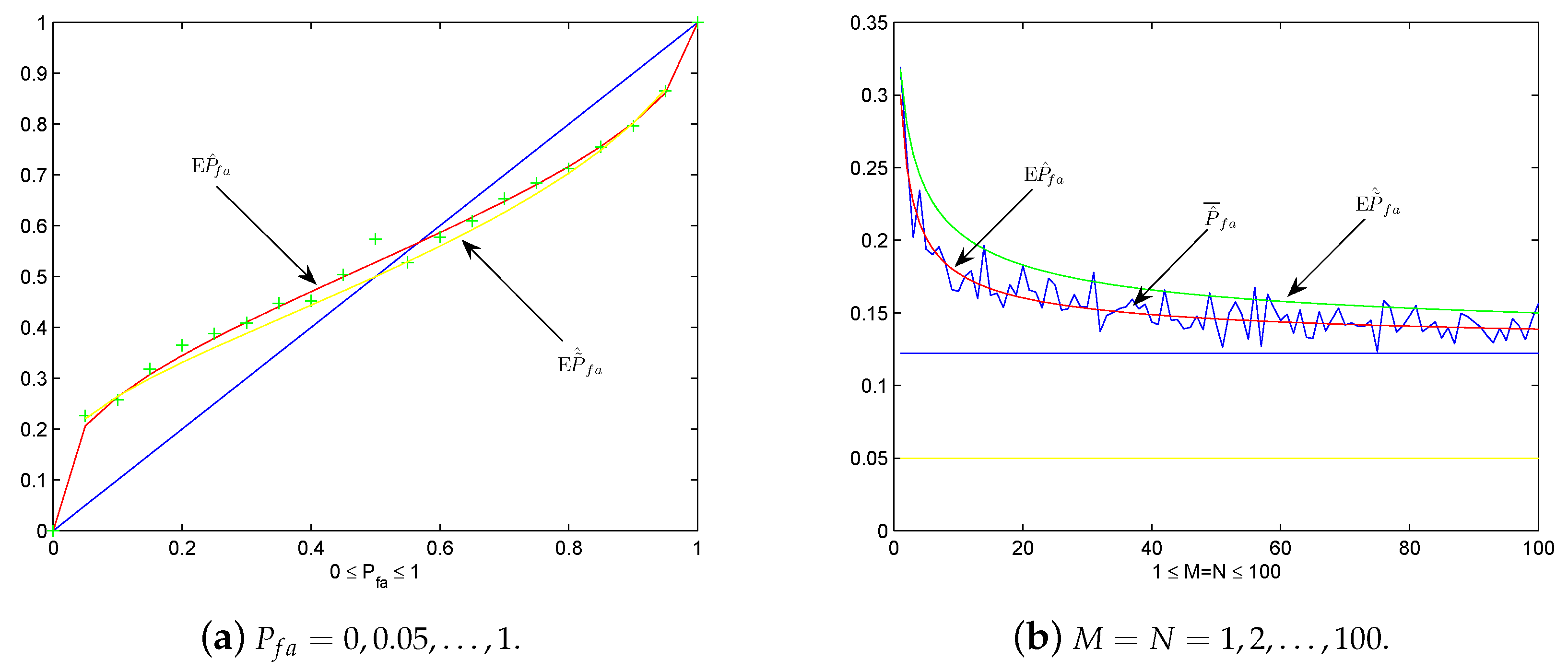
Now let us do some numerical experiments to detect the practicality of these theoretical results. Under the same setting of Example 1, we plot ${\overline{\widehat{P}}}_{fa}$ by ’+’, and $E{\widehat{P}}_{fa}$ and $E{\widehat{\tilde{P}}}_{fa}$ as the predesigned $P_{fa}\in [0,1]$ in Figure 3a. We see that $E{\widehat{P}}_{fa}$ serves better as the mean value of ${\overline{\widehat{P}}}_{fa}$ than $E{\widehat{\tilde{P}}}_{fa}$, which coincides with the fact that the latter is an approximating case. If $M,N$ is sufficiently large, $E{\widehat{\tilde{P}}}_{fa}$ approximates $E{\widehat{P}}_{fa}$ close as desired. Let us analyze more deeply the graphs in Figure 3a by the discovery in Remark 1. Let $M=\mu N$, the approximation of $E{\widehat{P}}_{fa}$ and $E{\widehat{\tilde{P}}}_{fa}$ is $Q(Q^{-1}\left(P_{fa}\right)/\sqrt{1+\mu })$ when $M=\mu N$ is large. Clearly, $Q(Q^{-1}\left(\frac{1}{2}\right)/\sqrt{1+\mu })=\frac{1}{2}$ by noticing $Q^{-1}\left(\frac{1}{2}\right)=0$. Graphically, this means the curves of $E{\widehat{P}}_{fa}$ and $E{\widehat{\tilde{P}}}_{fa}$ with respect to $P_{fa}\in [0,1]$ pass across the diagonal line in Figure 4 around $P_{fa}=\frac{1}{2}$ for sufficiently large $M,N$. If $M>>N$, i.e., $\mu$ close to 0, then $Q(Q^{-1}\left(P_{fa}\right)/\sqrt{1+\mu })\approx P_{fa}$. In this case, the graphs of $E{\widehat{P}}_{fa}$ and $E{\widehat{\tilde{P}}}_{fa}$ with respect to $P_{fa}\in [0,1]$ is close to the diagonal line.

Figure 3. The plot of ${\overline{\widehat{P}}}_{fa}$ by ’+’, $E{\widehat{P}}_{fa}$ and $E{\widehat{\tilde{P}}}_{fa}$ under setting of P_fa = 0, 0.05, …, 1 and M = N = 1, 2, …, 100. (a) The plot of ${\overline{\widehat{P}}}_{fa}$ by ’+’, $E{\widehat{P}}_{fa}$ and $E{\widehat{\tilde{P}}}_{fa}$ vs P_fa = 0, 0.05, …, 1. (b) The plot of ${\overline{\widehat{P}}}_{fa}$, $E{\widehat{P}}_{fa}$ and $E{\widehat{\tilde{P}}}_{fa}$ vs. $M=N=1,2,\dots ,100$, under P_fa = 0.05.

Figure 4. The plot of approximation of $E{\widehat{P}}_{fa}^2$ and $E{\widehat{\tilde{P}}}_{fa}^2$ and their upper bounds. (a) The plot of ${\overline{{\widehat{P}}^2}}_{fa}$ by ’+’, $\mathbf{B}({\widehat{P}}_{fa}^2)$ and $\mathbf{B}({\widehat{\tilde{P}}}_{fa}^2)$ vs. $P_{fa}$ = 0, 0.05, …, 1. (b) The plot of ${\overline{{\widehat{P}}^2}}_{fa}$ by ’+’, $\mathbf{B}({\widehat{P}}_{fa}^2)$ and $\mathbf{B}({\widehat{\tilde{P}}}_{fa}^2)$ vs. $M=N=1,\dots ,100$.

On the other hand, in Figure 3b we plot ${\overline{\widehat{P}}}_{fa}$, $E{\widehat{P}}_{fa}$ and $E{\widehat{\tilde{P}}}_{fa}$ under the same setting of Example 2 for $P_{fa}=0.05$. Again, we see that $E{\widehat{P}}_{fa}$ serves better as the mean value of ${\overline{\widehat{P}}}_{fa}$ than the approximation $E{\widehat{\tilde{P}}}_{fa}$. As $M=N$ changes from 1 to 100, $E{\widehat{P}}_{fa}$ and $E{\widehat{\tilde{P}}}_{fa}$ seem tend to the value of the upper straight line in Figure 3b, i.e., $Q(Q^{-1}\left(0.05\right)/\sqrt{2})=0.1124\cdots$, which justifies the observation in Remark 1.

In conclusion, the theoretical discoveries in the above four theorems and two remarks have been verified in these numerical experiments.

5. Upper Bounds of $\mathit{E}{\widehat{\mathit{P}}}_{\mathit{fa}}^{\mathbf{2}}$ and $\mathit{E}{\widehat{\tilde{\mathit{P}}}}_{\mathit{fa}}^{\mathbf{2}}$

After the calculations of $E{\widehat{P}}_{fa}$ and $E{\widehat{\tilde{P}}}_{fa}$, it is meaningful to have some information about the average deviations of ${\widehat{P}}_{fa}$ and ${\widehat{\tilde{P}}}_{fa}$ from their expectations. Technically, it is found very difficult to find explicit forms for $E{\widehat{P}}_{fa}^2$ and $E{\widehat{\tilde{P}}}_{fa}^2$ by existing special functions. We have to try to find some upper bounds instead. By the facts that ${\widehat{P}}_{fa}\in [0,1]$ and ${\widehat{\tilde{P}}}_{fa}\in [0,1]$, we have obvious upper bounds as

$$E{\widehat{P}}_{fa}^2\le E{\widehat{P}}_{fa}\le 1\mathrm{and}E{\widehat{\tilde{P}}}_{fa}^2\le E{\widehat{\tilde{P}}}_{fa}\le 1.$$

Thus, the more sharp upper bounds of $E{\widehat{P}}_{fa}^2$ and $E{\widehat{\tilde{P}}}_{fa}^2$ should be less than $E{\widehat{P}}_{fa}$ and $E{\widehat{\tilde{P}}}_{fa}$ respectively. For this target, let us list two propositions and two lemmas for technical preparation.

From the proofs of Theorems 1 and 3, we actually have the following two general results respectively.

Proposition 1.

For a real differentiable function $\psi :[0,\infty )\to [0,\infty )$,

$$\begin{array}{ll}\frac{d}{dx}& {\int }_0^{\infty }\mathsf{\Gamma }(m,t\psi \left(x\right))\frac{1}{\mathsf{\Gamma }\left(n\right)}{t}^{n-1}{e}^{-t}dt=-\frac{1}{B(n,m)}\frac{{\psi }^{m-1}\left(x\right){\psi }^{\prime }\left(x\right)}{{(1+\psi \left(x\right))}^{m+n}}\\ & =\frac{1}{B(n,m)}{\left(1-\varphi \left(x\right)\right)}^{m-1}{\left(\varphi \left(x\right)\right)}^{n-1}{\varphi }^{\prime }\left(x\right),\end{array}$$

(47)

where $\varphi \left(x\right)=\frac{1}{1+\psi \left(x\right)}$ and $m>0$, $n>0$.

Proposition 2.

For two real differentiable functions $\psi \left(x\right)$ and $\phi \left(x\right)$,

$$\begin{array}{cc}\hfill \frac{d}{dx}& {\int }_{R}Q(t\psi \left(x\right)+\phi \left(x\right))e^{-\frac{t^2}{2}}dt=-exp\left\{-\frac{{\phi }^2\left(x\right)}{2(1+{\psi }^2\left(x\right))}\right\}{\left(\frac{\phi \left(x\right)}{\sqrt{1+{\psi }^2\left(x\right)}}\right)}^{\prime }.\hfill \end{array}$$

(48)

We need two more inequalities regarding Gaussian and Gamma distributions respectively as follows. The proofs have been listed in Appendix A.

Lemma 1.

For $k\ge 1$ and $x>0$,

$$\begin{array}{c}\hfill {\mathsf{\Gamma }}^2(k,x)\le \mathsf{\Gamma }(k,2^{\frac{1}{k}}x).\end{array}$$

(49)

Lemma 2.

For $\forall x\in (-\infty ,+\infty )$,

$$\begin{array}{c}\hfill Q^2\left(x\right)<Q\left(\sqrt{2}x\right).\end{array}$$

(50)

By Proposition 1 and Lemma 1, we develop an upper bound for $E{\widehat{P}}_{fa}^2$ in the following.

Theorem 5.

Let $x={\mathsf{\Gamma }}^{-1}\left(M/2,P_{fa}\right)$, then an upper bound for $E{\widehat{P}}_{fa}^2$ is

$$\begin{array}{cc}\hfill \mathbf{B}\left({\widehat{P}}_{fa}^2\right)& \stackrel{\mathsf{\Delta }}{=}B\left(\frac{N}{N+2^{1+2/M}x},\frac{N}{2},\frac{M}{2}\right).\hfill \end{array}$$

(51)

Remark 3.

Note that

$$\begin{array}{c}\hfill 0<\frac{N}{N+2^{1+2/M}x}<\frac{N}{N+2x}\end{array}$$

for $x>0$, we know that the upper bound in (51) for $E{\widehat{P}}_{fa}^2$ is really lower than $E{\widehat{P}}_{fa}$.

Proof of Theorem 5.

By (25), we find an upper bound for the the expectation of squared probability of false alarm as

$$\begin{array}{ll}E{\widehat{P}}_{fa}^2& =E{\mathsf{\Gamma }}^2\left(\frac{M}{2},\frac{y}{{\sigma }_n^2}{\mathsf{\Gamma }}^{-1}\left(M/2,P_{fa}\right)\right)\\ & ={\int }_0^{\infty }{\mathsf{\Gamma }}^2\left(M/2,tx/N\right)f_{\chi }\left(t,N\right)dt,\end{array}$$

(52)

where we use the notations: $t=Ny/{\sigma }_n^2$ and $x={\mathsf{\Gamma }}^{-1}\left(M/2,P_{fa}\right)$. By Lemma 1, for $a\in (0,1)$ we derive

$$\begin{array}{ll}E{\widehat{P}}_{fa}^2& ={\int }_0^{\infty }{\mathsf{\Gamma }}^2\left(M/2,tx/N\right)f_{\chi }\left(t,N\right)dt\\ & \le {\int }_0^{\infty }\mathsf{\Gamma }(M/2,2^{2/M}tx/N)\frac{t^{N/2-1}{e}^{-t/2}}{2^{N/2}\mathsf{\Gamma }(N/2)}dt\stackrel{\mathsf{\Delta }}{=}\mathbf{B}\left({\widehat{P}}_{fa}^2\right).\end{array}$$

(53)

In order to use Proposition 1, introduce a transformation $u=t/2$. Then, we proceed (53) as

$$\begin{array}{cc}\hfill \mathbf{B}\left({\widehat{P}}_{fa}^2\right)& ={\int }_0^{\infty }\mathsf{\Gamma }\left(M/2,2^{1+2/M}tx/N\right)\frac{u^{N/2-1}{e}^{-u}}{\mathsf{\Gamma }(N/2)}du.\hfill \end{array}$$

(54)

Clearly, corresponding to Proposition 1, $\psi \left(x\right)=\frac{2^{1+2/M}x}{N}$ in (54). Thus, by Proposition 1, we derive

$$\begin{array}{c}\hfill \mathbf{B}\left({\widehat{P}}_{fa}^2\right)=B\left(\frac{N}{N+2^{1+2/M}x},\frac{N}{2},\frac{M}{2}\right).\end{array}$$

  □

By Proposition 2 and Lemma 2, we develop an upper bound for $E{\widehat{\tilde{P}}}_{fa}^2$ in the following.

Theorem 6.

Let $x=Q^{-1}\left(P_{fa}\right)$, then an upper bound for $E{\widehat{\tilde{P}}}_{fa}^2$ is

$$\begin{array}{c}\hfill \mathbf{B}\left({\widehat{\tilde{P}}}_{fa}^2\right)\stackrel{\mathsf{\Delta }}{=}Q\left(\frac{\sqrt{2}\beta x}{\sqrt{{\beta }^2+2{(x+\alpha )}^2}}\right)-Q\left(\beta \right),\end{array}$$

(55)

where $\alpha =\sqrt{M/2}$ and $\beta =\sqrt{N/2}$.

Remark 4.

Note that

$$\begin{array}{c}\hfill \frac{\sqrt{2}\beta x}{\sqrt{{\beta }^2+2{(x+\alpha )}^2}}>\frac{\beta x}{\sqrt{{\beta }^2+{(x+\alpha )}^2}}>0\end{array}$$

for $x>0$, we know that the upper bound in (55) for $E{\widehat{\tilde{P}}}_{fa}^2$ is really lower than $E{\widehat{\tilde{P}}}_{fa}$ for $P_{fa}\in [0,\frac{1}{2}]$.

Proof of Theorem 6.

Letting $x=Q^{-1}\left(P_{fa}\right)$, $t=(y-{\sigma }_n^2)/{\sigma }_n^2$, and recalling the notations $\alpha =\sqrt{M/2}$ and $\beta =\sqrt{N/2}$. By (24), we derive

$$\begin{array}{c}\hfill E{\widehat{\tilde{P}}}_{fa}^2={\int }_R{Q}^2(\alpha t+xt+x)\frac{\beta }{\sqrt{2\pi }}{e}^{-\frac{{\beta }^2{t}^2}{2}}dt.\end{array}$$

(56)

By Lemma 2, we proceed as

$$\begin{array}{cc}\hfill E{\widehat{\tilde{P}}}_{fa}^2& \le {\int }_{R}Q\left(\sqrt{2}(\alpha t+xt+x)\right)\frac{\beta }{\sqrt{2\pi }}{e}^{-\frac{{\beta }^2{t}^2}{2}}dt\stackrel{\mathsf{\Delta }}{=}\mathbf{B}\left({\widehat{\tilde{P}}}_{fa}^2\right).\hfill \end{array}$$

(57)

Introduce transformation $u=\beta t$, and thus $t=\frac{u}{\beta }$. Hence, we derive

$$\begin{array}{cc}\hfill \mathbf{B}\left({\widehat{\tilde{P}}}_{fa}^2\right)& ={\int }_{R}Q\left(\sqrt{2}\left[(\alpha +x)\frac{u}{\beta }+x\right]\right)\frac{e^{-\frac{u^2}{2}}}{\sqrt{2\pi }}du.\hfill \end{array}$$

(58)

Clearly, corresponding to Proposition 2, $\psi \left(x\right)=\sqrt{2}(\alpha +x)/\beta$ and $\phi \left(x\right)=\sqrt{2}x$. By the fact

$$\underset{x\to +\infty }{lim}\frac{\phi \left(x\right)}{\sqrt{1+{\psi }^2\left(x\right)}}=\underset{x\to +\infty }{lim}\frac{\sqrt{2}\beta x}{\sqrt{{\beta }^2+2{(x+\alpha )}^2}}=\beta$$

and Proposition 2, we have the formula (55).  □

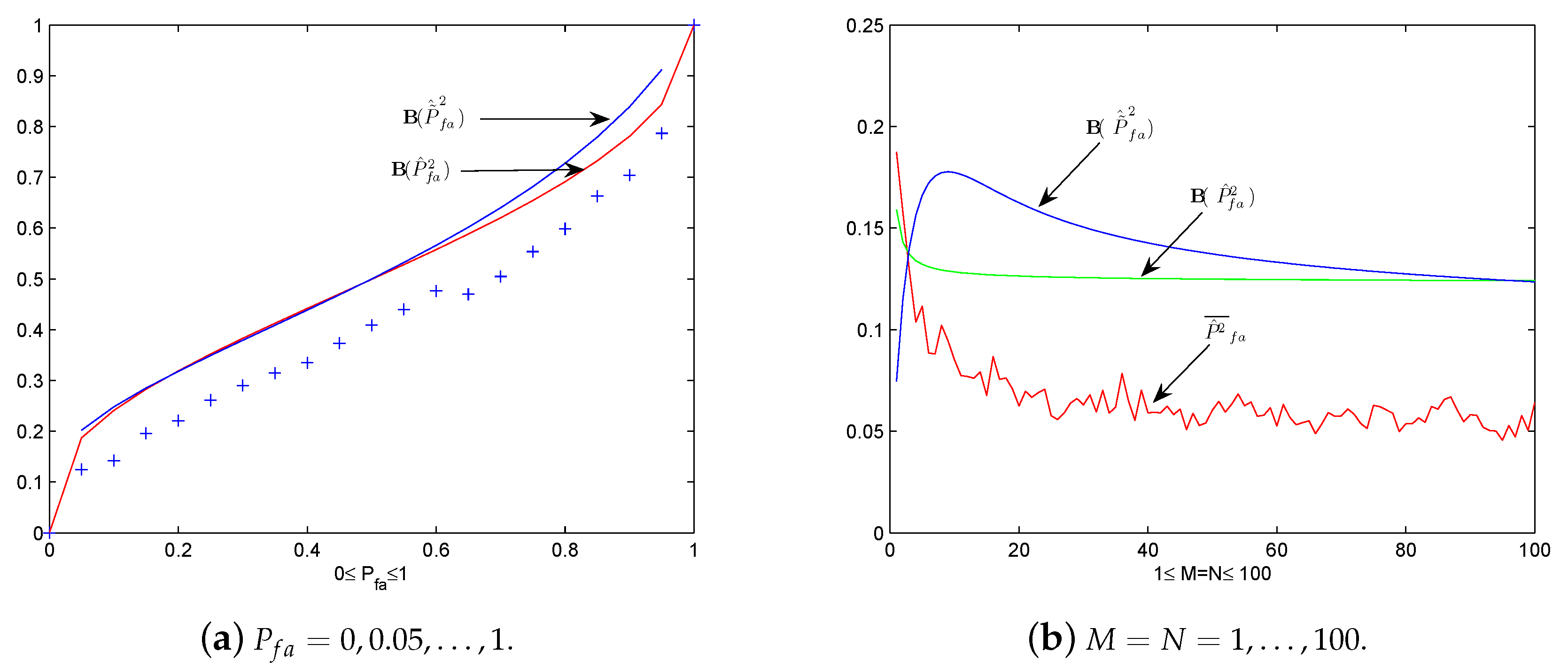
Now let us do two numerical experiments corresponding to examples in Section 3 to check how the two upper bounds work. The average squared false alarm probability is calculated over 600 sample paths by

$${\overline{{\widehat{P}}^2}}_{fa}=\frac{1}{600}\sum _{i=1}^{600}{\widehat{P}}_{fa}^2\left({\omega }_i\right)$$

to serve as an empirical approximation of $E{\widehat{P}}_{fa}^2$, where ${\widehat{P}}_{fa}\left({\omega }_i\right)$ denotes the calculated probability along the i-th sample path $\omega \left(i\right)$. Under the same setting of Example 1, we plot ${\overline{{\widehat{P}}^2}}_{fa}$ by ’+’, $\mathbf{B}({\widehat{P}}_{fa}^2)$ and $\mathbf{B}({\widehat{\tilde{P}}}_{fa}^2)$ as $P_{fa}$ changes from 0 to 1 in Figure 4a. It seems that $\mathbf{B}({\widehat{P}}_{fa}^2)$ is the better one, especially in the case $P_{fa}>\frac{1}{2}$. Under the same setting of Example 2, by letting $P_{fa}=0.05$ we plot ${\overline{{\widehat{P}}^2}}_{fa}$, $\mathbf{B}({\widehat{P}}_{fa}^2)$ and $\mathbf{B}({\widehat{\tilde{P}}}_{fa}^2)$ for $M=N=1,\dots ,100$ in Figure 4b. The two upper bounds seem not quite satisfied since both of them do not tend to ${\overline{{\widehat{P}}^2}}_{fa}$ as M (or N) tends to infinity.

6. New Thresholds Based on $E{\widehat{P}}_{fa}$ and $E{\widehat{\tilde{P}}}_{fa}$

In this section we derive new thresholds to guarantee the expectation $E{\widehat{P}}_{fa}=P_{fa}$ or in the approximation formula version, $E{\widehat{\tilde{P}}}_{fa}=P_{fa}$, by the help of Theorems 1 and 3, respectively.

The threshold ${\widehat{\lambda }}_{fa}$ given by (19) constructed by using estimated noise variance is actually a random variable itself. This leads to the fact that the resulted false alarm probability ${\widehat{P}}_{fa}$ given by (21) is generally different from the predesigned probability $P_{fa}$. It is found in Theorem 1 that the expected value of ${\widehat{P}}_{fa}$ is probably different from the predesigned probability $P_{fa}$. For instance, let $P_{fa}=0.05$ and $M=60$, $N=30$ as in Example 1, by Theorem 1,

$$\begin{array}{c}\hfill E{\widehat{P}}_{fa}=B\left(\frac{30}{30+2{\mathsf{\Gamma }}^{-1}\left(30,0.05\right)},15,30\right)=0.2065\cdots \end{array}$$

for the threshold given by (19), i.e., ${\widehat{\lambda }}_{fa}=\frac{2{\widehat{\sigma }}_n^2}{M}{\mathsf{\Gamma }}^{-1}\left(30,0.05\right),$ where ${\widehat{\sigma }}_n^2$ is estimated by $N=30$ independent observations. Obviously, the resulted expectation $E{\widehat{P}}_{fa}=0.2065\cdots$ is much bigger than the predesigned false alarm probability $P_{fa}=0.05$. This means the threshold is selected too low to guarantee the predesigned false probability $P_{fa}=0.05$ in an average sense. If we want the expectation $E{\widehat{P}}_{fa}=0.05$, the preassigned probability $P_{fa}^0$ for energy detection should be suitably smaller. Next we analyze how small the preassigned probability $P_{fa}^0$ should be and then derive a new threshold to guarantee $E{\widehat{P}}_{fa}=P_{fa}$.

For a given alarm level $P_{fa}$, say $0.05$, in order to derive a threshold to guarantee $E{\widehat{P}}_{fa}=P_{fa}$, it is found that the x in (26) should be

$$x=\frac{N}{2}\left(\frac{1}{B^{-1}(P_{fa},N/2,M/2)}-1\right)$$

by solve the target equation. Then by $x={\mathsf{\Gamma }}^{-1}\left(M/2,P_{fa}^0\right)$ described in Theorem 1, the preassigned initial threshold for energy detection should be $P_{fa}^0=\mathsf{\Gamma }\left(M/2,x\right)$. In other words, due to the fact that the noise variance is estimated by finite samples of noise, if we still want the false alarm rate less than $P_{fa}$, we may need to be more cautious to select the threshold for energy detection. For the simple example discussed above, i.e., $M=60$, $N=30$, if we want $E{\widehat{P}}_{fa}=0.05$, the preassigned false alarm rate should be approximately $P_{fa}^0=0.00033955$, which is much smaller than the desired rate $0.05$. However, if the sample number N increases to 100, the preassigned false alarm rate could be $P_{fa}^0=0.0129$. As the sample number N increases, the preassigned rate approaches to $0.05$ itself.

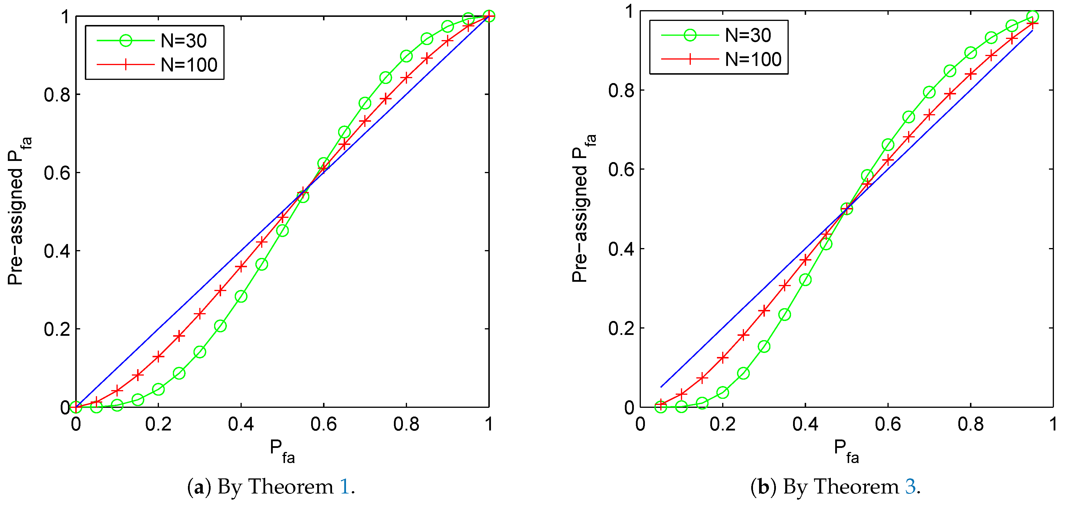
It is plotted in Figure 5a how the cautious preassigned false alarm rate $P_{fa}^0$ should be under the setting $M=60$ and $N=30,100$, for the sequence $P_{fa}=0,0.05,\dots ,1$. It is clearly shown in the figure that the preassigned false alarm rate $P_{fa}^0$ should be much smaller than the value $P_{fa}$ is designed to be. As the sample number N for estimation increases, the preassigned false alarm rate $P_{fa}^0$ approaches to the value of $P_{fa}$.

Figure 5. The plot of preassigned false alarm rate $P_{fa}^0$ to guarantee $E{\widehat{P}}_{fa}=P_{fa}$ and $E{\widehat{\tilde{P}}}_{fa}=P_{fa}$ by Theorems 1 and 3 respectively. (a) Preassigned rate derived by Theorem 1 to guarantee $E{\widehat{P}}_{fa}=P_{fa}$. (b) Preassigned rate derived by Theorem 1 to guarantee $E{\widehat{\tilde{P}}}_{fa}=P_{fa}$.

Consequently, by the value of x the derived new threshold is given by

$$\begin{array}{c}\hfill {\widehat{\lambda }}_{fa}^{new}=\frac{2{\widehat{\sigma }}_n^2}{M}x=\frac{N{\widehat{\sigma }}_n^2}{M}\left(\frac{1}{B^{-1}(P_{fa},N/2,M/2)}-1\right),\end{array}$$

(59)

where $B^{-1}(x,a,b)$ denotes the inverse function of $B(x,a,b)$. By formula (26), we have

$$\begin{array}{c}\hfill E(\mathrm{prob}[u>{\widehat{\lambda }}_{fa}^{new}])=P_{fa}.\end{array}$$

This means by this new threshold the expected false alarm probability is just the predesigned false alarm probability $P_{fa}$. Hence, this new threshold is more accurate to serve as CFAR threshold for energy detection when using estimated noise variance.

Similarly, for a given alarm level $P_{fa}$, say $0.05$, we derive a threshold to guarantee $E{\widehat{\tilde{P}}}_{fa}=P_{fa}$. Denote $\gamma =Q^{-1}(Q\left(\beta \right)+P_{fa})$. It can be solved by (26) that

$$x_{new}=\frac{\alpha {\gamma }^2+\beta \gamma \sqrt{\mathsf{\Delta }}}{{\beta }^2-{\gamma }^2}$$

with $\gamma =Q^{-1}(Q\left(\beta \right)+P_{fa})$, $\mathsf{\Delta }={\alpha }^2+{\beta }^2-{\gamma }^2$, $\alpha =\sqrt{M/2}$ and $\beta =\sqrt{N/2}$. Observe that $Q\left(\gamma \right)=Q\left(\beta \right)+P_{fa}>Q\left(\beta \right)$, it follows that $\gamma <\beta$. Then by $x=Q^{-1}\left(P_{fa}^0\right)$ stated in Theorem 3, it is clear that the preassigned false alarm rate should be $P_{fa}^0=Q\left(x_{new}\right)$. It is plotted in Figure 5b how the cautious preassigned false alarm rate $P_{fa}^0$ should be under the setting $M=60$ and $N=30,100$, for the sequence $P_{fa}=0.05,0.10,\dots ,0.95$. It is clearly shown in the figure that the preassigned false alarm rate $P_{fa}^0$ should be much smaller than the value $P_{fa}$ is designed to be. As the sample number N for estimation increases, the preassigned false alarm rate $P_{fa}^0$ approaches to the value of $P_{fa}$.

Consequently, by the value of $x_{new}$ the derived new threshold is given by

$$\begin{array}{c}\hfill {\widehat{\tilde{\lambda }}}_{fa}^{new}={\widehat{\sigma }}_n^2\left(1+\frac{x_{new}}{\sqrt{M/2}}\right).\end{array}$$

(60)

Then, by Theorem 3, we have

$$\begin{array}{c}\hfill E(\mathrm{prob}[u>{\widehat{\tilde{\lambda }}}_{fa}^{new}])=P_{fa}.\end{array}$$

Hence, this new threshold is much more accurate in an average sense than the empirical threshold simple replacement for energy detection when using estimated noise variance.

7. Conclusions

When using noise variance to set a CFAR threshold of energy detection for spectrum sensing, the derived threshold itself is a random variable. Thus, the resulted probability of false alarm is probably different from the predetermined false alarm probability $P_{fa}$. In this paper, we analyze some basic statistical properties of the resulted probability of false alarm ${\widehat{P}}_{fa}$ given by (21) and its approximating case ${\widehat{\tilde{P}}}_{fa}$ given by (24), and then some more suitable CFAR thresholds of energy detection are proposed. Specifically, we first deduce explicit descriptions for the expectations of ${\widehat{P}}_{fa}$ and ${\widehat{\tilde{P}}}_{fa}$ by Theorems 1 and 3 respectively in Section 4, and then some straightforward properties are established. These actually answer the first question we proposed in the introduction. Second, two upper bounds of $E{\widehat{P}}_{fa}^2$ and $E{\widehat{\tilde{P}}}_{fa}^2$ are derived by Theorems 5 and 6 respectively in Section 5, due to the difficulty to find exact explicit forms by known special functions. These answer the second question proposed in the introduction partially as well. Third, with the help of Theorem 3, the limitation of $E{\widehat{P}}_{fa}$ or $E{\widehat{\tilde{P}}}_{fa}$ for $M=\mu N$ as M or N tends to infinity is analyzed in Remark 1, which answers partly the third question in the introduction. Finally, new CFAR thresholds are proposed by assuring that $E{\widehat{P}}_{fa}$ or $E{\widehat{\tilde{P}}}_{fa}$ equals the predetermined false alarm probability $P_{fa}$ in Section 6. All analytical results derived in this paper are regarding the CFAR threshold. However, as a matter of fact, similar results hold for the CDR case.

For further consideration, it is of interest to describe explicitly $E{\widehat{P}}_{fa}^2$ and $E{\widehat{\tilde{P}}}_{fa}^2$. This means that a more cautious thresholds setting is possible. Observe that the CFAR and CDR thresholds are considered separately in this paper, it is crucial to consider CFAR and CDR thresholds synchronously in energy detection to achieve low false alarm probability and high detection probability simultaneously.