1. Introduction
This work aims to define the threshold value for selecting boundary nodes during jamming attacks. In wireless communication, there are two types of interference: intentional and unintentional interference. Unintentional interference is caused by nearby wireless devices, such as wi-fi, microwave, and Bluetooth signals. A jamming signal is an intentional interference utilizing the same tools to block the wireless channel or wireless device, intended to interrupt a wireless transmission and make a legitimate node unable to use network resources [
1]. Due to the shared communication medium of wireless sensor networks (WSNs), jammers efficiently disrupt the communication between nodes by emitting a signal towards the target channel using the same frequency band. The jamming signal harms the wireless channel based on the jammer’s position and transmitting power.
Jamming attacks are organized into two levels: the elementary and the advanced, based on the functionality and strategies used [
2]. The primary level includes constant jammers, deceptive jammers, and random jammers. A constant jammer transmits a random jamming signal continuously to make the target channel busy. All nodes inside the jammer’s transmission range are unable to access the channel to transmit data while the jammer is transmitting its signal. A deceptive jammer sends a regular signal, which leads all sensors near the jammer to switch to received mode until the jammer’s battery is depleted or the jammer is physically eliminated. A random jammer switches between sleep and active mode. The jammer blocks a communication channel for a random time and then turns to sleep mode. The time between sleep and transmit modes is unknown and is randomly selected by the jammer. The advanced level of jamming attacks use a proactive jammer. This kind of attack runs on a frequency domain. The jammer senses all possible channels. Once it detects a channel used by another node, it immediately emits a signal to jam it. The jammer adapts its frequency from one carrier to another, so it can block all channels. This type is difficult to detect because it uses the same method used in the frequency-hopping spread spectrum (FHSS) transmissions and direct-sequence spread spectrum (DSSS) transmissions.
Localizing a jammer in WSNs is necessary to improve existing countermeasures [
3]. WSNs are designed as multi-hop networks, in which each node forwards its collected data to the next hop node until reaching the sink node. The routing protocols need to determine the shortest path between the sender and the destination. When jamming attacks occur, the network topology is affected based on the jammer’s transmission range and the jammed region. The network topology is classified into three main types based on the jamming signal [
3]. Unjammed nodes are sensors located outside the jamming region and can transmit and receive data with neighbors. Boundary nodes may measure the jammer received signal strength (JRSS) directly from the jammer. They can communicate with unjammed and other boundary nodes. Jammed nodes are all sensors located inside the jamming region. These are entirely isolated from networks and cannot send or receive data from other sensors. All data sent to the jamming region fails to be received by the destination. A forced routing protocol is required to direct all data outside the jammed region and prevent resend requests and failed data delivery.
Tracking and localization algorithms are divided into range-free and range-base. Range-free algorithms utilize the geometric node’s position and the change of network topology to estimate jammer location. Centroid-based location (CL) and weighted centroid-based location (WCL) are examples of range-free location algorithms [
4,
5]. Both techniques are sensitive to the sensor’s location, the position of the jammer, and the density of nodes.
The existing boundary node selection algorithms are concerned with detecting nodes surrounding holes or the edge of the network. Based on our knowledge, there has been no research conducted to detect boundary nodes during jamming attacks.
Hsieh [
6] introduced the Distributed Boundary Recognition Algorithm (BNST RA) to locate boundary nodes distributed around the hole and the network border. The algorithm is based on four levels. First, the author implemented the Virtual Hexagonal Landmark (VHL) to choose Closure Nodes (CNs) found close to the hole and on the border of the network, becoming landmark nodes (LNs). Second, all CNs join and are dubbed Coarse Boundary Cycles (CBCs). Each CBC is then assigned a unique ID to define each hole. Third, all boundaries circling the hole are connected. Fourth, the boundary availability is checked by sending a message to all 1-hop neighbors waiting for a reply.
Khan [
7] proposed a Self-Detection Boundary Recognition (SDBR) which examines every node as if it has a closed cycle or a broken path. For the closed cycle, each node constructs a 2-hop neighbor, selecting any node and then moving in one direction to reach the starting point. If this node is a closed path, then it will mark the internal node. Otherwise, it is marked as a boundary node.
Dabba [
8] proposed a Border Coverage Protocol (BCP) consisting of three steps. First, the nodes close to the network boundary are detected. Each node broadcasts its location, ID, and sensing range to the base station nodes on the border. Second, all nodes selected in the previous step send the message to their one-hop neighbors. Any node receiving this message mark becomes a transfer node. Third, the boundary nodes selected in the first step are replaced by transfer nodes, which are then considered the new boundary nodes.
In this paper, we have proposed a method to select boundary nodes. Selected boundary nodes have the responsibility of catching the JRSS. We applied an extended Kalman filter to estimate the position of the jammer at each time step. We utilized the signal-to-noise ratio to define boundary nodes while the jammer is moving.
2. Materials and Method
This work aimed to define the threshold value for selecting boundary nodes during jamming attacks. SNR is the difference between the signal received and the unwanted noise, including the jamming signal [
9], since the jammer’s signal itself is considered noise. SNR is measured in decibels (dB). SNR thresholds are determined by the wireless carrier, as these are system-designed. If the SNR is below the threshold value, the bit error rate (BER) increases, packet delivery ratio (PDR) decreases, and the system fails to decode the signal. It discards the signal and requests retransmission. The jammer is intended to lower the SNR below the threshold value, which disrupts communication between transceivers. Nodes closer to the jammer have a lower SNR, and the amount of SNR decreases until it drops below the threshold value, becoming a jammed node. Based on this observation, we designed an algorithm to compute another threshold value, called the boundary node selection threshold (BNST). The BNST is calculated based on a node’s location, sensing range, and the JRSS.
The SNR, including the jamming signal, then becomes:
wherein
is the power received by the node,
is the noise floor, and
is the jammer’s received signal.
This work examines the path loss model. When signals propagate between a transmitter and receiver, they are affected by the surrounding environment. There are many factors that attenuate the signal while traveling through space, such as reflection, diffraction, refraction, and absorption [
10]. The path loss model is usually expressed in decibels (dB) and described as follows:
The path loss is represented by
, and
is the path loss exponent, which varies by environment. Typically, the path loss exponent is between 2 and 4, based on the types of metal and objects affecting the signal as it propagates from the sender to the receiver. Variable
is the distance between the transmitter and the receiver. Therefore, the power received by a node becomes the following:
where
is constant and depends on antenna characteristics. is the node’s transmission range measured at the reference distance. is a zero-mean Gaussian distributed random variable. Variables i and j are identifiers for the nodes.
In this network model, we assume that all nodes are randomly deployed and remain unchanged. Sensors have equal transmit power and are equipped with omnidirectional antenna. The data reach their destinations through a multi-hop network, in which each node forwards its collected data to its neighbors. Each node in the network is assumed to have a table of its neighbors’ identification and locations. A constant jammer was adopted in this work and implemented using an omnidirectional antenna and fixed transmit power. Because our focus was selecting boundary nodes and tracking, we assumed all jammed nodes would be detected, and the system would know their location and identification.
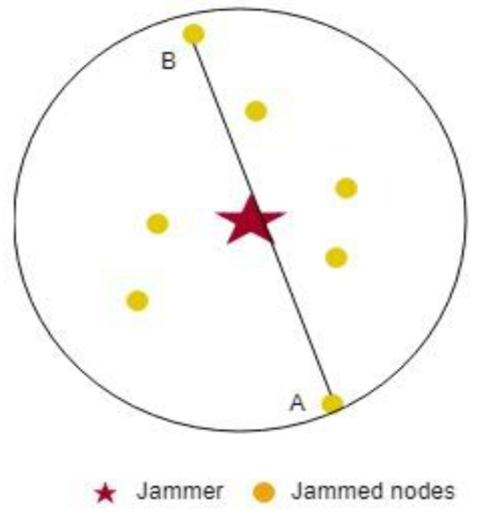
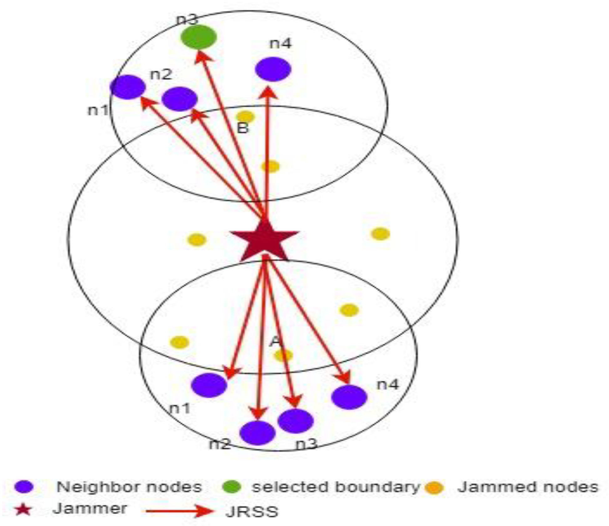
We calculate BNST as follows. After the jammer begins to function, the jammed node locations are denoted as
, where
is the number of jammed nodes. To find the maximum distance between two jammed nodes, the Euclidean distance is used to compute the distance between all nodes inside the jammer region (see Equation (5) above). Therefore, the maximum distance between two nodes becomes
, where
is the maximum distance and
are the two jammed nodes’ identification. In
Figure 1, above, (a,b) are the two selected nodes with maximum distance.
Next, we find the farthest neighbor from each selected node using the same method of computing the max distance between two jammed nodes. The red circle
is selected as a reference node to define the BNST as follows:
is the minimum power that could be received by nodes at the maximum distance, where SR is the node’s sensing range. We used this value to compute the largest SNR at that point. At the first iteration, we select BNST as the maximum value. If the BNST computed at
time step is larger than the selected BNST, the BNST at the first iteration is set to the maximum BNST. Any node with an SNR lower than the BNST value can capture the JRSS. Each node computes the average SNR and compares it to the system threshold and BSNT. If the average SNR is between the system threshold and the BNST, then the nodes become boundary nodes by themselves. Boundary nodes continue to update their average SNR, and when it drops below the threshold or rises above the BNST, the node will stop tracking the jammer.
where
is the total of neighbor nodes,
is the power received from neighbor
is the JRSS at node
. The extended Kalman filter is based on a recursive approach, and it is used in this paper to estimate the jammer position. It is suitable for nonlinear state estimation, and it consists of two main processes: the prediction and update states [
11]. The state transition model can be expressed as:
where
expresses the state vector and
the process noise, with
a covariance matrix with zero mean and normal distribution
. In addition,
represents the state transition for nonlinear equations. The measurement vector is expressed as:
where
is the measurement noise with covariance
and have normal distribution with zero mean. The nonlinear function is represented by h, and H is the Jacobian matrix. The prediction and update states are expressed as:
We apply EKF to validate our algorithm. The position-velocity model is used to track the jammer under constant acceleration [
12]. The jammer location is denoted by
, and the velocity is
. Therefore, the state vector is expressed as:
The measurement vector becomes:
The observation function and the Jacobian matrix are described as follows:
where
and
is the jammer transmission power at reference distance
3. Results
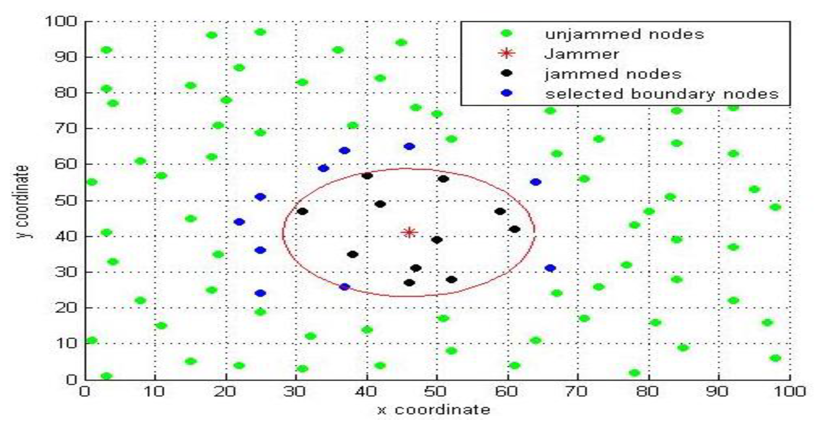
To evaluate the performance of the suggested algorithm, 100 sensors were randomly deployed on an area 100 × 100 m. The jammer moved randomly, starting at point 40, 30 before constantly accelerating. The transmission range of the sensors was 15 m. The jammer had a transmission range of 17 m. The transmission power was set to −36 dBm and −35 dBm for the nodes and jammer, respectively. The noise floor was about −95 dBm and the SNR threshold value was 21.8, as presented in
Figure 3.
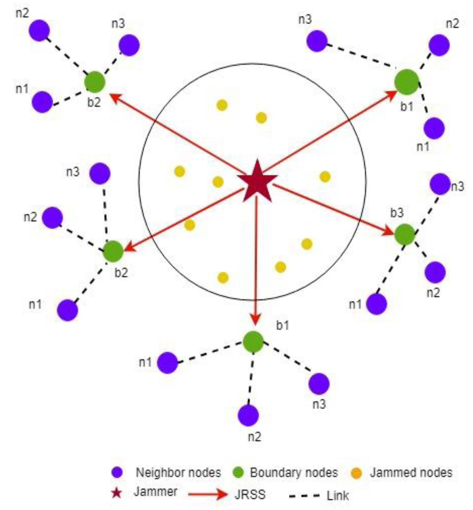
Figure 4 shows the jammer, and the nodes within the jammer’s transmit range are isolated and affected by the jammer’s signal.
The red star is the jammer, the yellow circles represent the jammed nodes, green circles are the boundary nodes, and the blue circle denotes the boundary nodes’ neighbors. The red arrow is the JRSS received by the boundary node, and the dotted line is the bidirectional link between nodes.
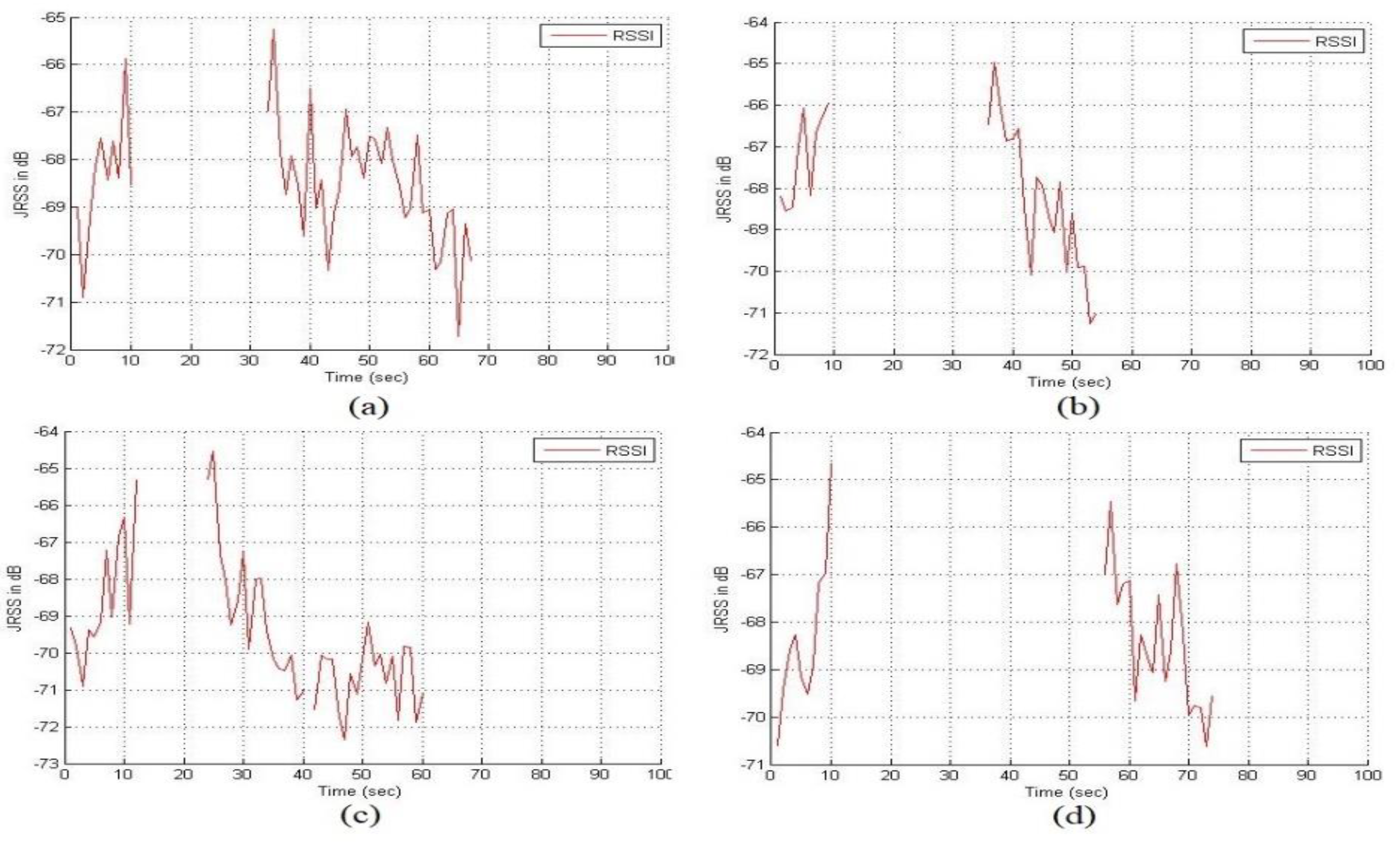
It is clear that the nodes located outside the jamming region are affected by JRSS. When the jammer is moving, the status of the node changes from unjammed to jammed, or a jammed node becomes an isolated node, as shown in
Figure 5.
This illustration represents boundary nodes affected during jammer movement. In (a), the node detects JRSS at t = 0 and becomes a jammed node in the period from t = 11 s to t = 23 s. In this period, we lost the jammer information. For the same reason, in b, c, and d, the boundary nodes are missing the tracking information while the jammer changes its position. The system stops tracking for the first time when encountering missing data, which t = 11 s shows in
Figure 6. For this analysis, defining the boundary nodes while the jammer moving is mandatory. The unjammed nodes received the JRSS as noise, and the SNR decreased based on the amount of JRSS received by the node. Based on this observation, we defined a new threshold for boundary node selection.
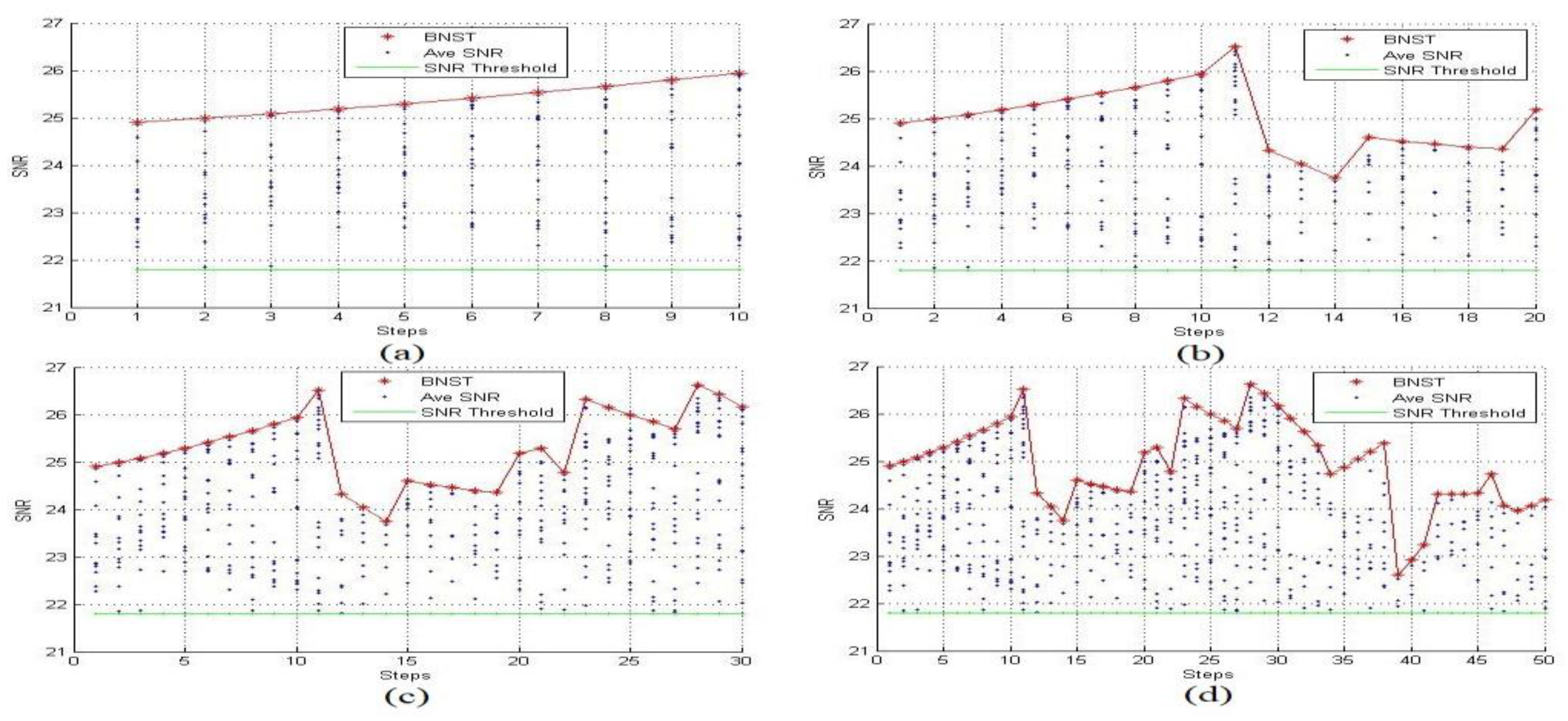
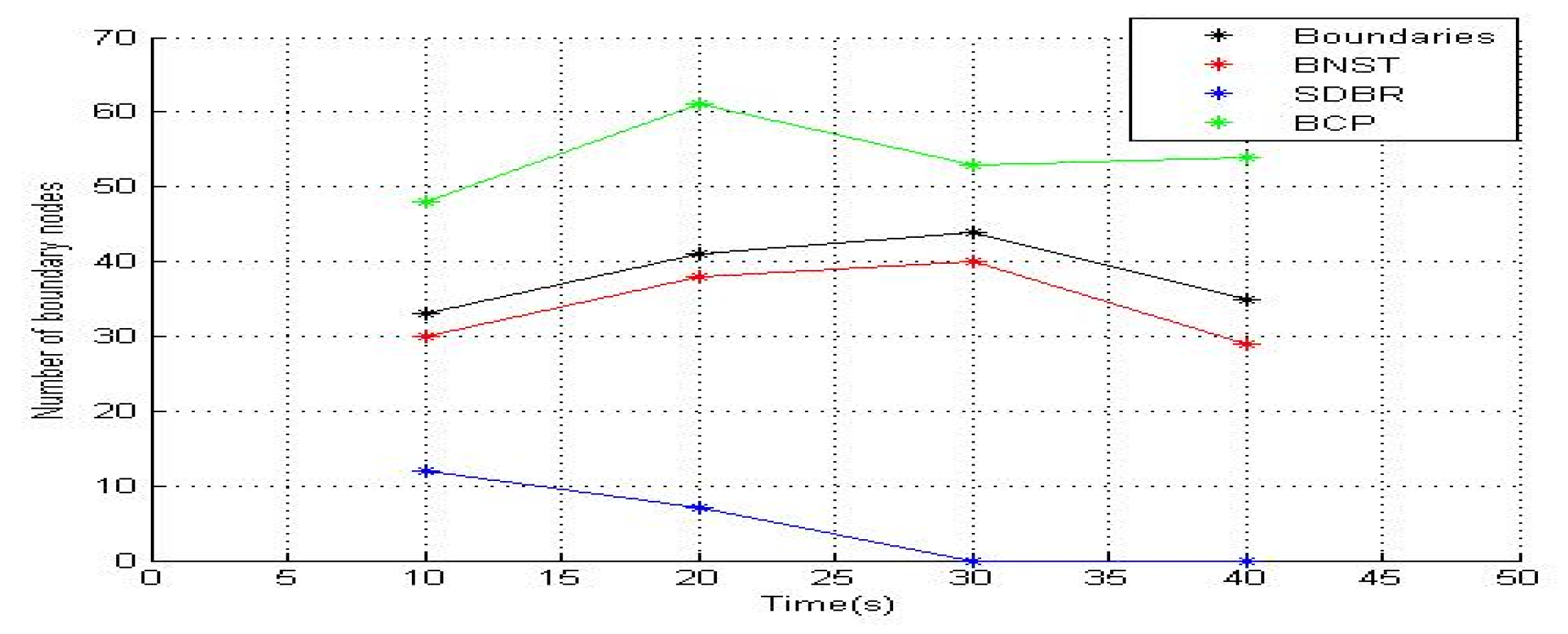
We examined the BNST at time steps 10 s, 20 s, 30 s, and 50 s.
Figure 7 represents the average SNR measured by each sensor.
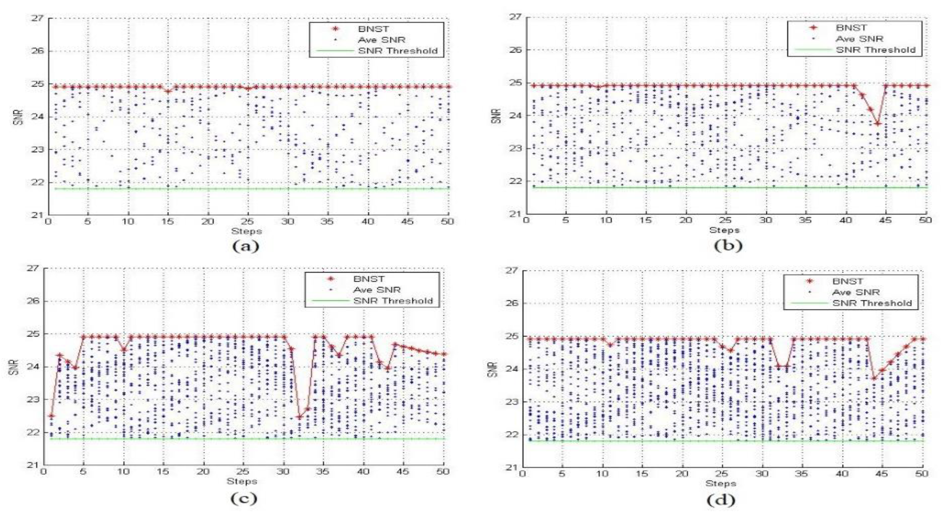
Figure 8 shows the BNST estimated with different jammer’s transmission range 15 m, 20 m, 30 m and 35 m.
As described in the previous section, all nodes estimate the average SNR and match it with the system threshold, or the SNR threshold and BNST value. If the computed value falls between two these values, the sensor turns itself into a boundary node and begins tracking the jammer until its average SNR drops below the SNR threshold or rises above the BNST value. In
Figure 7a, there are ten nodes that became boundary nodes by themselves and starting to read the JRSS. At time step 17 in (b), four elected boundary nodes had an average SNR between the SNR threshold and the BNST.
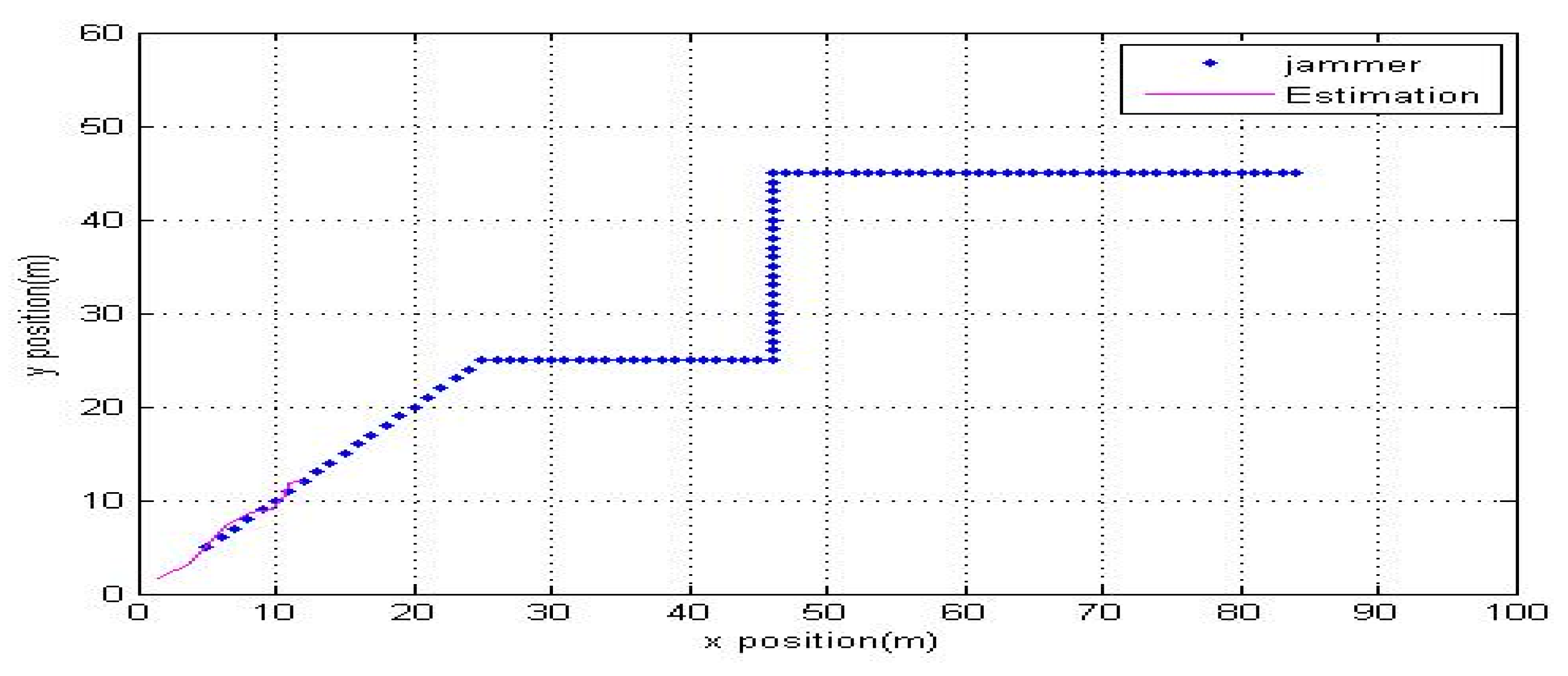
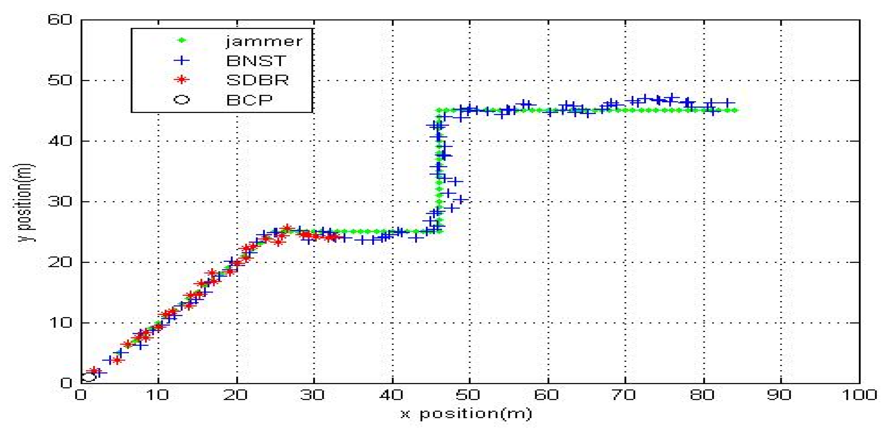
Figure 9 shows the jammer’s estimated location and its real position, found by applying EKF to measure the JRSS by selected boundary nodes at every time step.
In this study, we compared BNST with SDBR and BCP. Unlike SDBR and BCP, because BNST does not depend on four neighboring locations and nodes degrees, BNST performed better and had a higher efficiency at detecting nodes whose transmission ranges intersected with the jammer’s transmission range. As shown in
Figure 9, at the time step of 10 s, 32 nodes were present around the jammer field, and they could catch JRSS. Please note that BNST recognized 30 nodes, SDBR recognized 12 nodes, and BCP recognized 45 nodes, including those nodes that were incorrectly detected. Because SDBR is based on nodes degree and limited to be equal to or larger than six nodes, it fails to recognize boundary nodes that have less than six nodes on the second hop. Because of the random deployment, location of nodes, transmission range, and neighboring nodes, BCP defined any nodes that had less than four nodes on each side as boundary nodes. BCP was successful in detecting all boundary nodes. Note that nodes that are located far away from the jamming region with their transmission range not intersecting with the jammer transmission range and having less than four neighbors on each side are defined as boundary nodes. Therefore, the number of boundary nodes detected by BCP is always larger than that by BNST and SDBR. When the jammer is closer to the network center, SDBR failed to locate any boundary nodes because the jammer is positioned around the center. Moreover, because of the jamming effect, all nodes deployed around the edge of the network lost most of their neighbors.
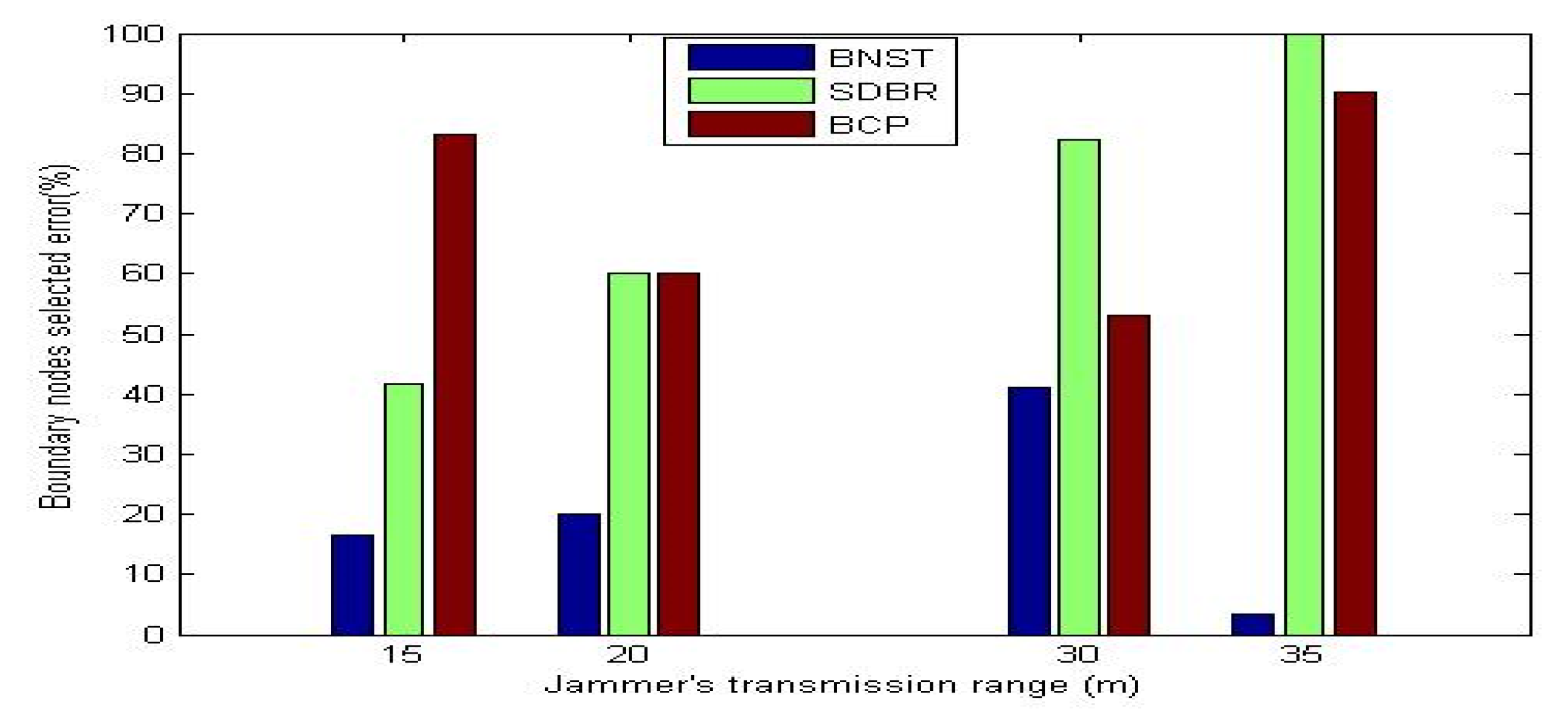
Figure 10 shows the percentage error of the selected boundary nodes when the jammer’s transmission range was adjusted to 15 m, 20 m, 30 m, and 35 m. Note that BNST has a higher efficiency and fewer boundary nodes recognition errors compared to SDBR and BCP. As shown in
Figure 10, when the jammer’s transmission range was adjusted to 35 m, which indicates more jammed nodes and a longer jamming region was covered by the jammer, SDBR failed to detect the boundary nodes. However, EKF is designed to receive tracking data at each time step by all the detected boundary nodes. As shown in
Figure 11, EKF stopped tracking the jammer at t = 32 s because SDBR failed to detect the boundary nodes and EKF did not receive any data. When applied to BCP, EKF failed to track the enemy at all times because there are certain boundaries that were wrongly selected and there was no data feed provided to EKF. However, BNST detected most boundary nodes, and when this data was provided to EKF, it could track the jammer and detect its location at each time step.


